Sage Journals: Discover world-class research

Abstract

Backdrivability is a key characteristic of robotic reducers; however, a long-standing lack of theoretical research has constrained its engineering application. Hysteresis, as an inherent characteristic of reducers, can effectively reflect the dynamic behavior during rotational motion. This paper systematically studies the backdrivability of reducers based on hysteresis characteristics. Combining the practical needs of robotic applications, the definition of back drive is clarified, emphasizing that its core lies in the rotation angle and energy absorption capacity. By establishing a correlation model between hysteresis characteristics and backdrivability, generalized polynomial and analytical expressions are proposed: lost motion is introduced as a key indicator, utilizing numerical changes in the hysteresis curve to evaluate the rotation angle; the area enclosed by the hysteresis curve is used to characterize the energy absorption capacity of the reducer during back drive, and statistical analysis methods along with torque-energy curves are employed to evaluate overall and instantaneous energy consumption performance, respectively. Experiments compared the backdrivability of two reducers made of different materials. The results indicate that geometric errors, elastic deformation, and material properties all significantly influence back-driving behavior.

Keywords

back driving hysteresis curve reducer energy dissipation analysis

Introduction

When robots interact with humans or the surrounding environment, such as encountering impacts or collisions, good backdrivability can impart compliance to the robot, enhancing safety in human-robot interaction.^1–4 This is particularly important in scenarios assisting users, such as lower-limb wearable robots,^5,6 upper extremity exoskeleton robots,⁷ and wearable robots for carrying heavy loads.⁸ These scenarios often require the use of joint torque sensors to detect contact forces, protecting the user’s safety through torque feedback and closed-loop control.^9–11 However, in most cases, due to cost and size constraints, torque sensors are not installed in the joints. Consequently, when encountering sudden large impacts, the control system cannot provide corresponding feedback control, failing to guarantee human-robot interaction safety. Therefore, it is particularly necessary to enhance the joint’s ability to buffer external impacts when the robot lacks the ability to perceive environmental torque information.^12–14

The reducer is the core actuating component for motion control in robot joints, and its performance directly affects the overall machine performance.^15,16 Literature¹⁷ defines back drive as “the ease with which a force applied to the output shaft of a power transmission mechanism causes motion to be transmitted from the output shaft back to the input shaft.” Literature^18,19 considers back-driving force as “the ability of a joint to receive power from the external environment.” Literature¹¹ defines back-driving capability as “the ability to absorb energy from the external environment.” From these definitions, it can be seen that if a reducer has sufficient back-driving capability, it can quickly reverse and absorb external energy when subjected to impact or collision, thereby protecting the robot and the user. Current research on backdrivability mainly focuses on optimizing system design or improving control algorithms. How to study the backdrivability of the reducer itself is an issue that needs consideration.

A comprehensive review of the current state of back-drive research reveals the following: Firstly, although there is research on joint backdrivability from a control perspective, this method is not suitable for reducers themselves, and research methods specifically for their backdrivability are relatively lacking. Secondly, the requirements for reducer backdrivability are unclear, leading to missing relevant concepts or definitions. Thirdly, using the reverse starting torque as an indicator for evaluating backdrivability²⁰—for example, the smaller the reverse starting torque, the stronger the backdrivability—is common. However, the back drive of a reducer involves complex core issues such as energy conversion, energy transfer, and motion control. The reverse starting torque is a single-property indicator and has the problem of incomplete reflection. Therefore, to study the backdrivability of a reducer, it is most important to combine the reducer’s own motion characteristics, identify suitable comprehensive indicators, and conduct research based on them.

Summarizing the concept of back drive and related research, for reducers, the essence of back drive is the reverse impact of load torque fluctuation on the reducer. This includes two core factors: load torque fluctuation and energy absorption and dissipation at the output end. Hysteresis is a physical phenomenon widely existing in nature and man-made systems.^21,22 Reducers are typical systems with hysteresis characteristics.²³ The presence of hysteresis causes the output shaft to lag in rotation angle when the direction of input shaft movement changes. The hysteresis curve is typically used to reflect the hysteresis characteristics of a reducer.²⁴ The hysteresis curve not only fully reflects the relationship between system torque and rotation angle but also its area is closely related to the energy dissipation of the reducer.²⁵ This characteristic is significant for understanding the back-driving mechanism and characterization of reducers. Therefore, this paper will analyze the impact of hysteresis on backdrivability based on the study of reducer hysteresis characteristics, propose a research method for reducer backdrivability, and provide its testing and evaluation methods. This aims to guide reducer design, understand the variation law of backdrivability, and provide reference for its engineering applications.

Concept of back drive

The principles of forward drive and back drive for a reducer are shown in Figure 1. Contrary to forward drive, the back drive mode of a reducer occurs when the reducer is subjected to impact or collision: power is input from the output end of the reducer, transmitted through the internal transmission mechanism, and output to the input end.

Figure 1.

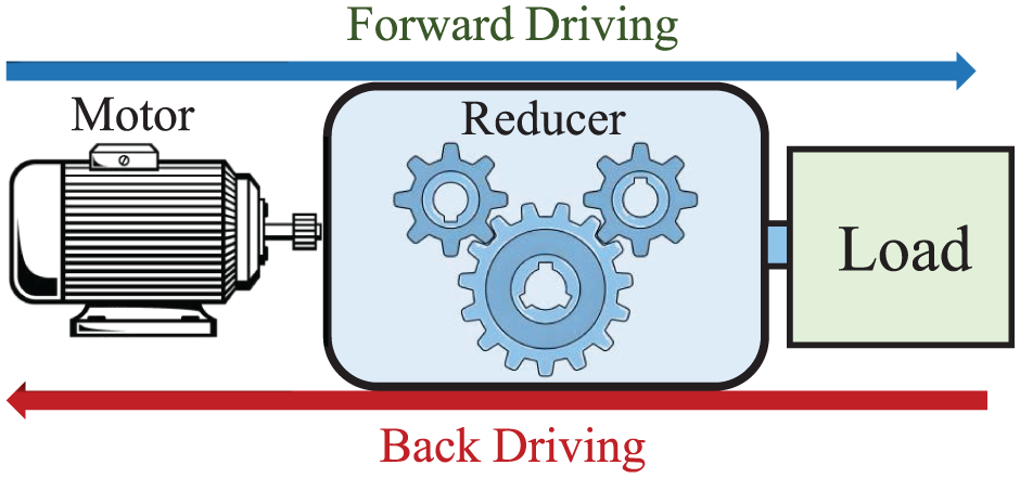
Forward driving and back-driving process of a robot reducer.

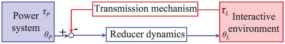
Based on the current needs for back drive in reducers, we can define back drive as follows: when a reducer encounters external impact or collision and needs to perform back drive, it must possess two capabilities: rapid reversal and absorption of external energy. Therefore, the back drive of a reducer can be defined as: “The ability to undergo rapid reversal and absorb external energy upon an abrupt change in the output-end load torque.” This definition can be represented by equation (1) and Figure 2. In the equation, B represents the backdrivability of the reducer, W_L is the energy absorbed by the system during the back-driving process, and θ_L is the rotation angle at the output end corresponding to the energy W_L absorbed by the reducer during the back-driving process. In the figure, τ and θPP are the torque and rotation angle at the input end of the reducer, and τ_L is the load torque. Furthermore, all the characters mentioned in the text are summarized in Table 1 in the Appendix, along with detailed explanations.

B = H (θ_{L}, W_{L})

(1)

Figure 2.

Principle of reducer hysteresis.

Hysteresis of the reducer

Concept of hysteresis

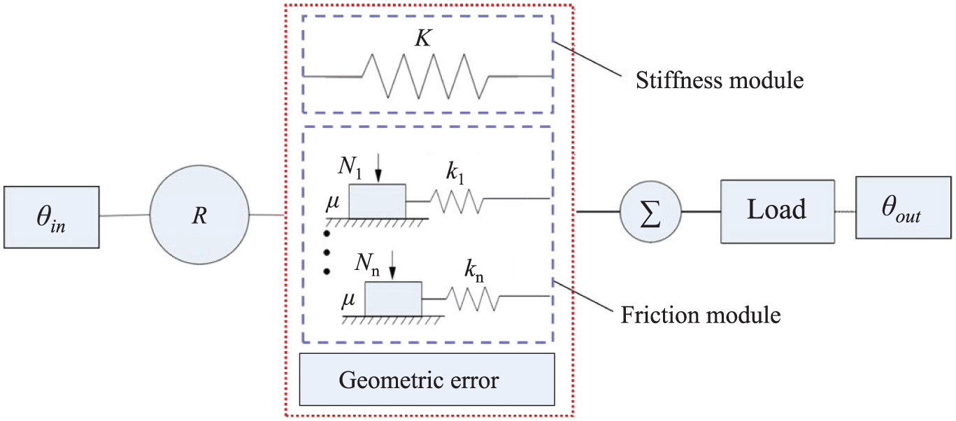
The hysteresis model of a reducer is shown in Figure 3. It consists of a geometric error module, a friction module, and a stiffness module, meaning hysteresis is the coupled result of these three components’ hysteresis. In the figure, θ_in is the input rotation angle, θ_out is the output rotation angle, R is the reduction ratio of the reducer, K represents the stiffness of the reducer, μ is the friction coefficient, and N is the normal force.

Figure 3.

Reducer hysteresis model.

According to the literature,²⁶ let the output rotation angle of the reducer be $θ_{out} (τ, \overset{\cdot}{τ})$ , where τ is the output torque and $\overset{\cdot}{τ}$ is the loading rate. The corresponding curve is shown in Figure 4. It is formed by the superposition of θ_g(τ) generated by geometric error, $θ_{out} (τ, \overset{\cdot}{τ})$ generated by friction, and θ_e(τ) generated by elastic deformation, which can be expressed by formula (2).

θ_{out} (τ, \overset{\cdot}{τ}) = {\begin{matrix} θ_{g +} (τ) + θ_{f +} (τ, \overset{\cdot}{τ}) + θ_{e +} (τ) + \frac{θ_{in}}{R}, \overset{\cdot}{τ} > 0 \\ θ_{g -} (τ) + θ_{f -} (τ, \overset{\cdot}{τ}) + θ_{e -} (τ) + \frac{θ_{in}}{R}, \overset{\cdot}{τ} < 0 \end{matrix}

(2)

Figure 4.

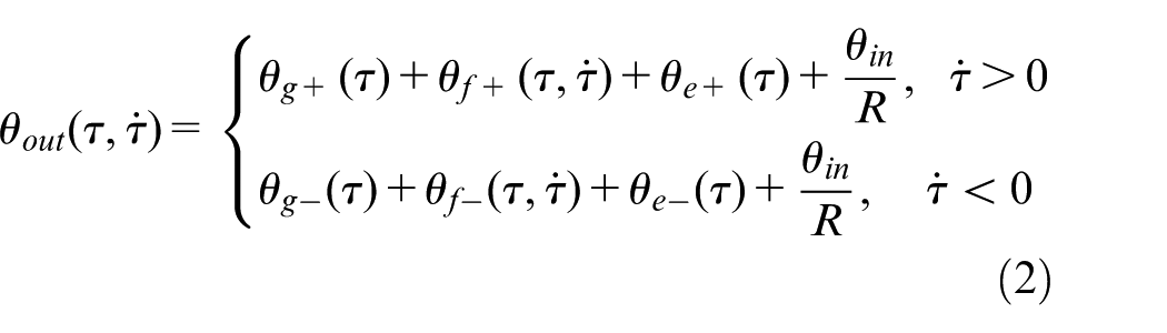
Composition of the reducer hysteresis curve.

It can be further expressed by equation (3):

θ_{out} (τ, \overset{\cdot}{τ}) = θ_{g} (τ) + θ_{f} (τ, \overset{\cdot}{τ}) + θ_{e} (τ) + \frac{θ_{in}}{R}

(3)

The evaluation of reducer hysteresis characteristics falls into two categories: first, numerical evaluation based on the hysteresis curve, reflecting hysteresis characteristics through the rotation angle; second, focusing on changes in the morphological parameters of the hysteresis curve, such as the area S enclosed by the hysteresis curve and the energy dissipation ratio u indicator. The area enclosed by the hysteresis curve is defined as S, which is proportional to the dissipated energy of the reducer, reflecting its energy dissipation capacity. The energy dissipation ratio u is an indicator measuring the energy utilization efficiency of the reducer. It is the ratio of the energy dissipated by the reducer in one loading-unloading cycle of the hysteresis curve to the total absorbed strain energy, as shown in Figure 5. In the figure, the hysteresis curve is composed of the ascending curve $θ_{out +}$ , the descending curve $θ_{out -}$ and the mean curve $θ_{out_m}$ , T_r represents the rated torque of the reducer, the sum of the areas $S_{Δ AFB}$ and $S_{Δ CDE}$ represents the total absorbed strain energy. u is expressed by formula (4).

u = \frac{S}{S_{Δ A F B} + S_{Δ C D E}} \times 100 %

(4)

Figure 5.

Morphological characteristic parameters of the hysteresis curve.

Characterization method for backdrivability

The core factors of reducer back drive are the angle of rotation at the output end and the energy absorbed during the output rotation process. Hysteresis affects both of these aspects, and the loading rate within hysteresis is directly related to load fluctuation during the back-driving process. Assuming a fixed speed or torque change rate condition, the rotation angle during back drive can be expressed using the hysteresis curve as:

θ_{b} = θ_{out} (τ, \overset{\cdot}{τ})

(5)

Similarly, to evaluate the ability of the reducer to absorb external impact energy during reversal, based on the characteristics of hysteresis, the area S enclosed by the hysteresis curve and the energy dissipation ratio u can be used, as shown in equation (6).

W_{b} = (S (τ, \overset{\cdot}{τ}), u (τ, \overset{\cdot}{τ}))

(6)

Further, equation (1) can be expressed as equation (7).

B = H (θ_{out} (τ, \overset{\cdot}{τ}), S (τ, \overset{\cdot}{τ}), u (τ, \overset{\cdot}{τ}))

(7)

In summary, the study of reducer backdrivability can be analyzed using the hysteresis characteristics of the reducer. A detailed analysis follows below.

Rotation angle in back drive

Factors influencing rotation angle

When conducting hysteresis testing on a reducer, the method of fixing the input end and loading the output end is usually adopted. At this time, the input rotation angle θ_in is 0. Thus, equation (3) can be expressed as equation (8).

θ_{out} (τ, \overset{\cdot}{τ}) = θ_{e} (τ) + θ_{f} (τ, \overset{\cdot}{τ}) + θ_{g}

(8)

The function of $\overset{\cdot}{τ}$ can be expressed as equation (9), where t is the loading time.

\overset{\cdot}{τ} = \overset{\cdot}{τ} (t)

(9)

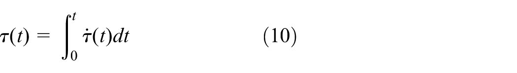
Then, the output torque τ can be expressed as equation (10):

τ (t) = \int_{0}^{t} \overset{\cdot}{τ} (t) dt

(10)

Let the area enclosed by $θ_{f} (τ, \overset{\cdot}{τ})$ be $S_{f} (t)$ . Then, $θ_{f} (τ, \overset{\cdot}{τ})$ can be expressed as equation (11):

θ_{f} (τ, \overset{\cdot}{τ}) = \frac{d S_{f} (t)}{d τ (t)}

(11)

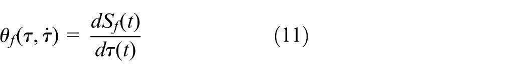
Substituting equations (10) and (11) into equation (8), the analytical expression for the hysteresis curve is obtained:

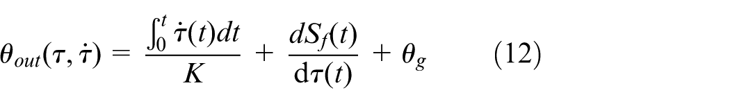
θ_{out} (τ, \overset{\cdot}{τ}) = \frac{\int_{0}^{t} \overset{\cdot}{τ} (t) dt}{K} + \frac{d S_{f} (t)}{d τ (t)} + θ_{g}

(12)

From equation (12), it can be seen that the loading rate, stiffness, friction, and geometric error of the reducer all affect the magnitude of the rotation angle.

Evaluation method for rotation angle

Lost motion δ is a key indicator characterizing the hysteresis phenomenon in reducers. It represents the lag in the rotation angle of the output end from when the direction of movement at the input end changes until the output end follows the change in direction. Therefore, based on the previous analysis, lost motion can be used to reflect the rotation angle during back drive. Its evaluation method is shown in Figure 6.

Figure 6.

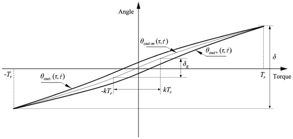
Evaluation method of lost motion.

δ is as shown in equation (13), where T_r is the rated torque of the reducer, and k represents the coefficient selected for δ_g, which is influenced by factors such as reducer manufacturing and installation. It is usually specified based on actual requirements.

δ = f_{m} (T_{r}) - f_{m} (T_{r})

(13)

Energy analysis and evaluation in back drive

Back-driving energy model

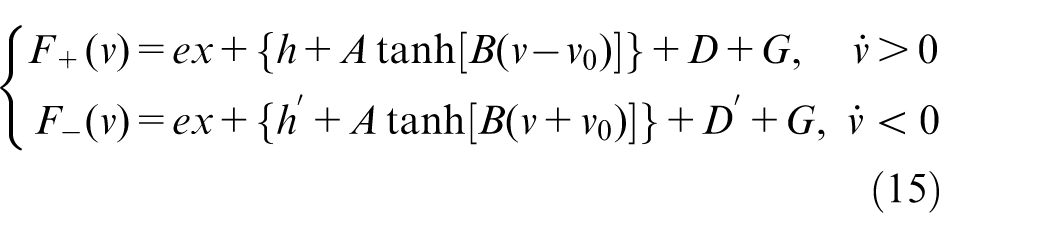
The hysteresis curve of the reducer is parameterized using linear and hyperbolic functions. Based on equation (3), a parameterized expression for the output rotation angle and torque is established. Let v be the input excitation, F(v) the output response, e the stiffness, A and B coefficients, D the geometric error, and G the ratio of the input rotation angle to the reduction ratio. The expression is shown in equation (14).

F (v) = ev + A \tanh (B \cdot v) + D + G

(14)

Furthermore, the expressions for the rising curve F ₊ (v) and the falling curve F ₊ (v) are obtained as equation (15).

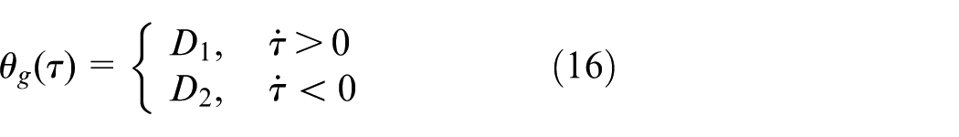
{\begin{matrix} F_{+} (v) = ex + {h + A \tanh [B (v - v_{0})]} + D + G, \overset{\cdot}{v} > 0 \\ F_{-} (v) = ex + {h^{'} + A \tanh [B (v + v_{0})]} + D^{'} + G, \overset{\cdot}{v} < 0 \end{matrix}

(15)

According to the functional form of the hysteresis curve, the rotation angle caused by geometric error hysteresis can be represented by a constant. Therefore, θ_g(τ) can be expressed by equation (16).

θ_{g} (τ) = {\begin{matrix} \begin{matrix} D_{1}, & \overset{\cdot}{τ} > 0 \end{matrix} \\ \begin{matrix} D_{2}, & \overset{\cdot}{τ} < 0 \end{matrix} \end{matrix}

(16)

The output torque of the stiffness module can be expressed as an odd function of the rotation angle. Hence, θ_e(τ) can be represented using a Taylor series, as shown in equation (17).

θ_{e} (τ) = k_{1} τ + k_{3} τ^{3} + k_{5} τ^{5} + \dots + k_{2 n - 1} τ^{2 n - 1}

(17)

Equation (17) is simplified into a polynomial form, as shown in equation (18).

θ_{e} (τ) = i τ + j τ^{3} + q τ^{5}

(18)

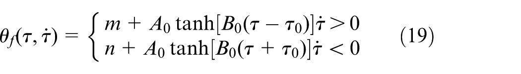
The rotation angle caused by frictional hysteresis in the reducer is represented using a hyperbolic function, as shown in equation (19).

θ_{f} (τ, \overset{\cdot}{τ}) = {\begin{matrix} m + A_{0} \tanh [B_{0} (τ - τ_{0})] \overset{\cdot}{τ} > 0 \\ n + A_{0} \tanh [B_{0} (τ + τ_{0})] \overset{\cdot}{τ} < 0 \end{matrix}

(19)

Substituting equations (15), (16), (18), and (19) yields the parametric equation of the reducer’s hysteresis curve, as shown in equation (20).

θ_{out} (τ, \overset{\cdot}{τ}) = {\begin{matrix} i_{0} τ + j_{0} τ^{3} + q_{0} τ^{5} + {m + A_{0} \tanh [B_{0} (τ - τ_{0})]} + D_{1} + G, \overset{\cdot}{τ} > 0 \\ i_{0} τ + j_{0} τ^{3} + q_{0} τ^{5} + {n + A_{0} \tanh [B_{0} (τ + τ_{0})]} + D_{2} + G, \overset{\cdot}{τ} < 0 \end{matrix}

(20)

Based on equation (20), the area enclosed by the hysteresis curve can be calculated, as shown in equation (21), and the energy calculation is shown in equation (22).

S = \int_{- τ_{R}}^{τ_{R}} θ_{out -} (τ, \overset{\cdot}{τ}) d τ - \int_{- τ_{R}}^{τ_{R}} θ_{out +} (τ, \overset{\cdot}{τ}) d τ

(21)

W = \frac{S}{r}

(22)

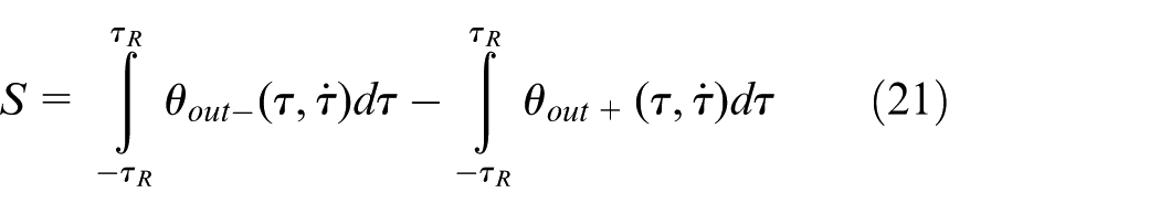
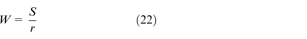
In the equations, r is the radius of the reducer’s output shaft. Additionally, S can also be expressed as equation (23), where S_g and S_e are the areas of the hysteresis curves caused by geometric error and elastic deformation, respectively.

S = S_{g} + S_{f} + S_{e}

(23)

S _g reflects the energy consumed by the reducer to overcome geometric error during reversal. Larger geometric errors result in more energy consumed by the reducer and a larger enclosed area. S_f reflects the energy consumed by the reducer to overcome internal and external friction during reversal. It is related to the contact area, wear rate, and average friction coefficient during reducer operation. Stronger friction leads to more energy consumed by the reducer, larger S_f, and a wider and thicker $θ_{f} (τ, \overset{\cdot}{τ})$ curve. S_e reflects the energy consumed when elastic deformation occurs in the reducer. It is related to the reducer’s material and the applied load. Stronger elastic deformation results in larger S_e.

Energy evaluation method

The evaluation methods for the energy absorption capacity of reducer back drive can be divided into two types: First, based on the total area S enclosed by the hysteresis curve and the energy dissipation ratio u, which reflect the reducer’s energy absorption capacity during one reversal process. Second, obtaining the reducer’s torque-energy curve from the hysteresis curve, which reflects the reducer’s energy absorption capacity at a specific instantaneous torque.

The first evaluation method can use statistical analysis. Specifically, extreme values and mean values are used to evaluate the area S and the energy dissipation ratio u. S_max, S_min, $\bar{S}$ , u_max, u_min, $\bar{u}$ are the maximum value, minimum value, and mean value of the evaluation indicators S and u, as shown in equations (24) and (25).

{\begin{matrix} S_{max} = MAX {S (i)} \\ S_{min} = MIN {S (i)} \\ \bar{S} = \frac{1}{m} \sum_{i = 1}^{m} S (i) \end{matrix}

(24)

{\begin{matrix} u_{max} = MAX {u (i)} \\ u_{min} = MIN {u (i)} \\ \bar{u} = \frac{1}{m} \sum_{i = 1}^{m} u (i) \end{matrix}

(25)

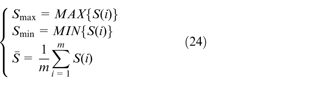
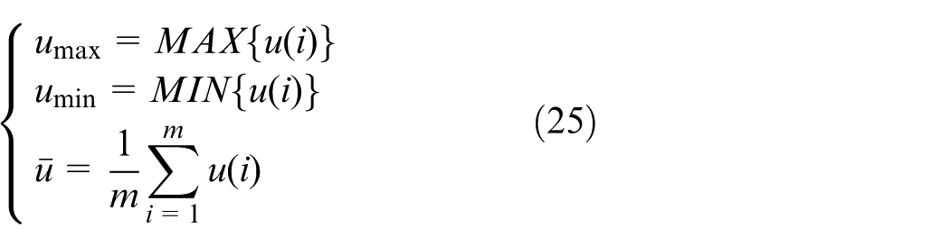
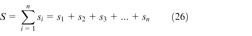
In the formula, m represents the number of sampling points. The second evaluation method is based on the integral method. To calculate the area enclosed by the hysteresis curve shown in Figure 7, according to the definition of integration, the interpolation method can be used to divide the rising and falling curves into several equal parts, calculate the area of each part, and sum them up, as shown in equation (26).

S = \sum_{i = 1}^{n} s_{i} = s_{1} + s_{2} + s_{3} + . . . + s_{n}

(26)

Figure 7.

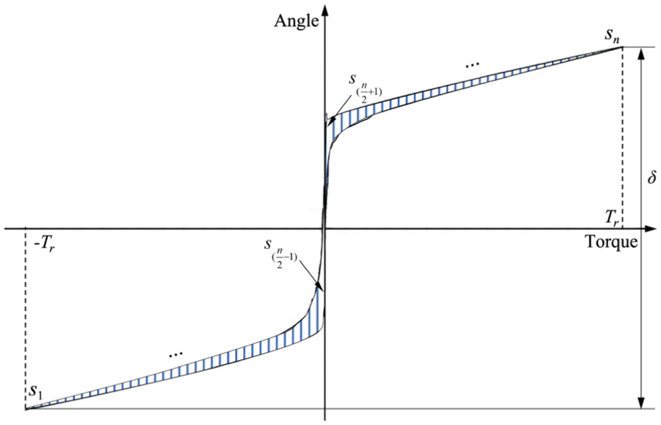
Area enclosed by the hysteresis curve.

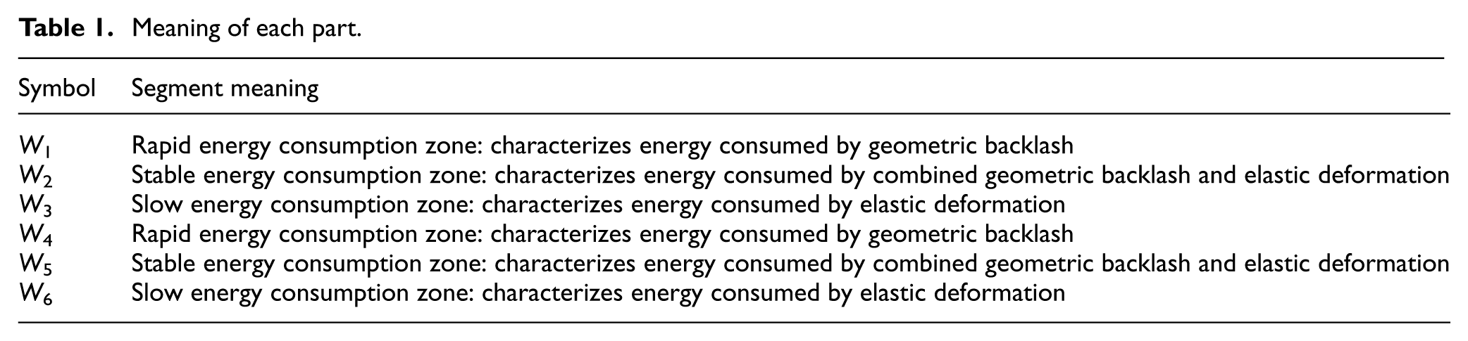
In the formula, n represents the number of integration units. Therefore, based on Figure 6 and equation (26), the correspondence between the area and different torque levels can be established using the integral method, that is, the energy absorption amount corresponding to different torque levels. The resulting torque-energy curve is shown in Figure 8, the meaning of each segment is shown in Table 1, and the curves for each part are expressed by equation (27).

{\begin{matrix} W_{1} (τ_{1}) = \frac{\int_{0}^{τ_{1}} [f_{-} (τ) - f_{+} (τ)] d τ}{r} \\ W_{2} (τ_{2}) = \frac{\int_{τ_{1}}^{τ_{2}} [f_{-} (τ) - f_{+} (τ)] d τ}{r} \\ W_{3} (T_{r}) = \frac{\int_{τ_{2}}^{T_{r}} [f_{-} (τ) - f_{+} (τ)] d τ}{r} \\ W_{4} (τ_{3}) = \frac{\int_{τ_{3}}^{0} [f_{-} (τ) - f_{+} (τ)] d τ}{r} \\ W_{5} (τ_{4}) = \frac{\int_{τ_{4}}^{τ_{3}} [f_{-} (τ) - f_{+} (τ)] d τ}{r} \\ W_{6} (- T_{r}) = \frac{\int_{T_{r}}^{τ_{4}} [f_{-} (τ) - f_{+} (τ)] d τ}{r} \end{matrix}

(27)

Table 1.

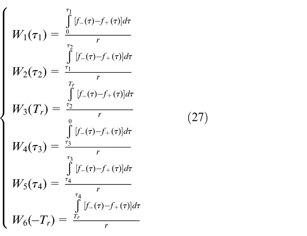
Meaning of each part.

Symbol	Segment meaning
W ₁	Rapid energy consumption zone: characterizes energy consumed by geometric backlash
W ₂	Stable energy consumption zone: characterizes energy consumed by combined geometric backlash and elastic deformation
W ₃	Slow energy consumption zone: characterizes energy consumed by elastic deformation
W ₄	Rapid energy consumption zone: characterizes energy consumed by geometric backlash
W ₅	Stable energy consumption zone: characterizes energy consumed by combined geometric backlash and elastic deformation
W ₆	Slow energy consumption zone: characterizes energy consumed by elastic deformation

Figure 8.

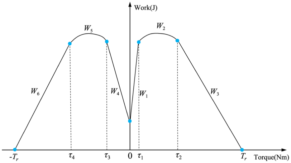
Torque-energy curve.

Experimental research

Testing equipment

The testing equipment is illustrated in Figure 9. The test system comprises a precision mechanical subsystem, a hardware subsystem, and dedicated testing software. An industrial control computer drives the load motor via a fieldbus-controlled driver to achieve high-precision torque regulation. A rotary encoder continuously monitors the rotational angle at the reducer’s output shaft in real time, while a torque sensor simultaneously measures the corresponding output torque. Data are acquired at a sampling frequency of 1 kHz and transmitted to the industrial control computer through the fieldbus interface.

Figure 9.

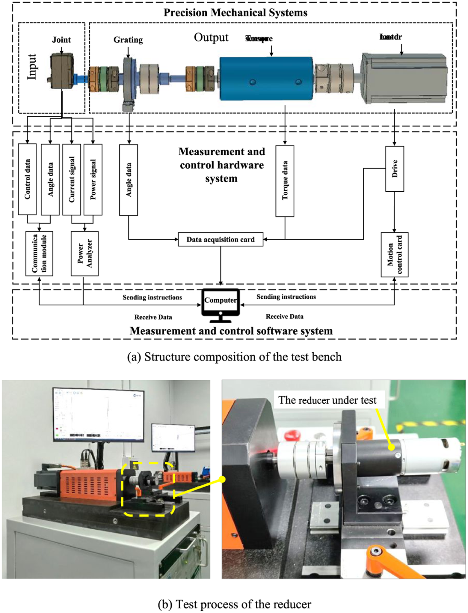
Reducer test bench and test scenario: (a) structure composition of the test bench and (b) test process of the reducer.

During testing, the reducer’s input shaft is fixed, and the output shaft is subjected to a controlled loading sequence according to a preset loading rate (0.01, 0.05, or 0.1 Nm/s). Specifically, the output shaft is first loaded positively—that is, in the forward direction—up to the rated torque T_r, then gradually unloaded back to zero; subsequently, it is loaded negatively—that is, in the reverse direction—up to the rated torque T_r, followed again by unloading to zero; finally, it is reloaded positively to T_r.

The testing software processes the raw measurement data—including filtering and calibration—according to established test standards, generates corresponding plots, and ultimately produces the reducer’s hysteresis curve.

Model fitting accuracy analysis

The small reducer employed in the tests is illustrated in Figure 10. This unit is a planetary gear reducer with a nominal diameter of 38 mm and a reduction ratio of 64. The sun gear is fabricated from powder metallurgy, while the first and second planetary gears are made of plastic; the third planetary gear is also produced via powder metallurgy. The internal surface of the metallic housing features an integral ring gear. The rated output torque of the reducer is 3 Nm.

Figure 10.

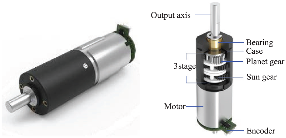
The physical and structural diagrams of the tested small reducer.

The small reducer depicted in the figure underwent controlled loading tests. During single-cycle loading up to the rated torque of 3 Nm, the applied torque ramp rate was maintained at 0.05 Nm/s. Both the ascending (loading) and descending (unloading) torque–displacement curves were fitted using the least-squares method; the resulting fitting parameters are summarized in Table 1, and the corresponding fitting performance is presented in Figure 11.

Figure 11.

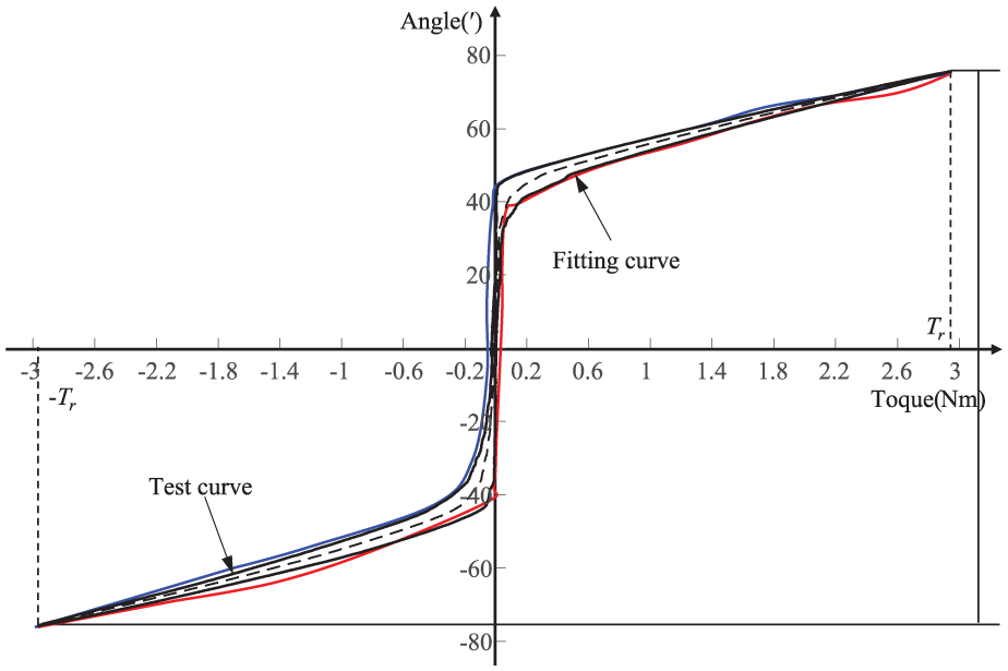
Test curve and fitting curve.

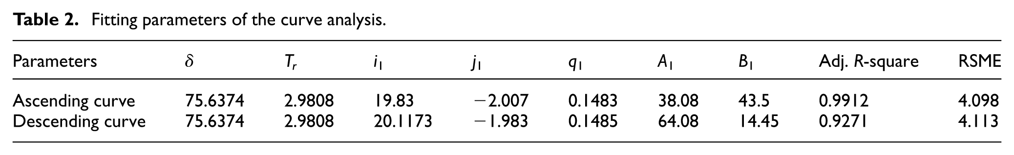
As shown in Table 2, both the ascending and descending curves exhibit a high degree of fit quality. As evident from Figure 11, however, relatively larger discrepancies between the fitted hysteresis curve and the experimentally measured hysteresis curve occur under high-load conditions. Further analysis indicates that these deviations primarily stem from minor slippage at the output shaft interface when high torque is applied. Nevertheless, the overall curve-fitting accuracy remains satisfactory.

Table 2.

Fitting parameters of the curve analysis.

Parameters	δ	T _r	i ₁	j ₁	q ₁	A ₁	B ₁	Adj. R-square	RSME
Ascending curve	75.6374	2.9808	19.83	−2.007	0.1483	38.08	43.5	0.9912	4.098
Descending curve	75.6374	2.9808	20.1173	−1.983	0.1485	64.08	14.45	0.9271	4.113

Backdrivability analysis

Back-driving angle variation

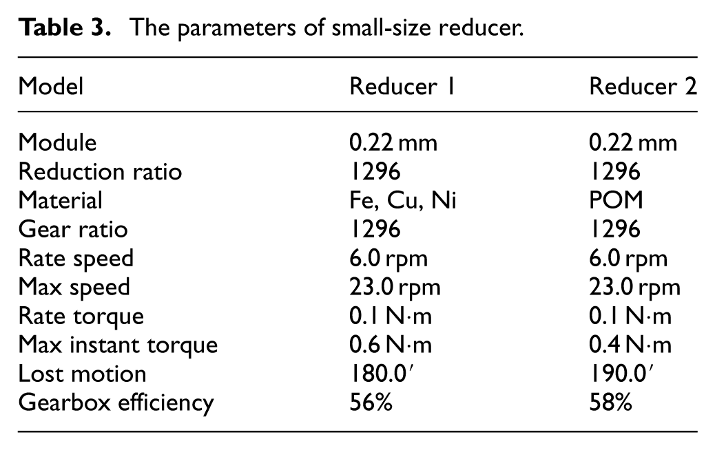
An experimental study was conducted on two small-sized planetary reducers used in robots. The reducers use 0.22 mm module spur gears with a four-stage planetary transmission. The physical objects and structure are shown in Figure 12. The gear material for Reducer 1 is powder metallurgy, and for Reducer 2, it is plastic. Other specifications are the same to neglect the influence of the reduction ratio. Specific parameters are shown in Table 3.

Figure 12.

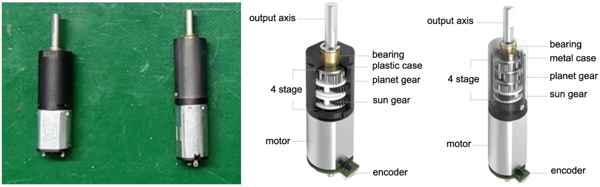
Tested small reducer: (a) the physical diagrams of Reducer 1 (right) and Reducer 2 (left) and (b) the internal structure of Reducer 1 (right) and Reducer 2 (left).

Table 3.

The parameters of small-size reducer.

Model	Reducer 1	Reducer 2
Module	0.22 mm	0.22 mm
Reduction ratio	1296	1296
Material	Fe, Cu, Ni	POM
Gear ratio	1296	1296
Rate speed	6.0 rpm	6.0 rpm
Max speed	23.0 rpm	23.0 rpm
Rate torque	0.1 N·m	0.1 N·m
Max instant torque	0.6 N·m	0.4 N·m
Lost motion	180.0′	190.0′
Gearbox efficiency	56%	58%

Reducers 1 and 2 were tested at loading rates of 0.01, 0.05, and 0.1 Nm/s up to 0.1 Nm to simulate the backdrivability of the reducers under different impact scenarios. Among these, 0.05 Nm/s corresponds to the default loading rate in hysteresis testing. The obtained hysteresis curves are shown in Figures 13 and 14.

Figure 13.

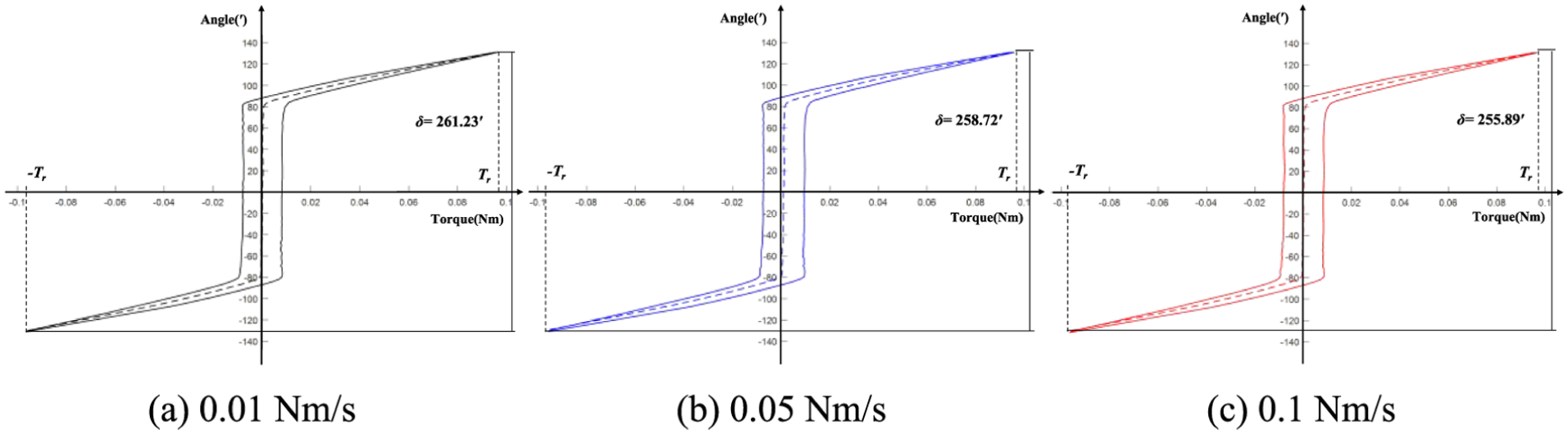
Hysteresis curves of Reducer 1: (a) 0.01 Nm/s, (b) 0.05 Nm/s, and (c) 0.1 Nm/s.

Figure 14.

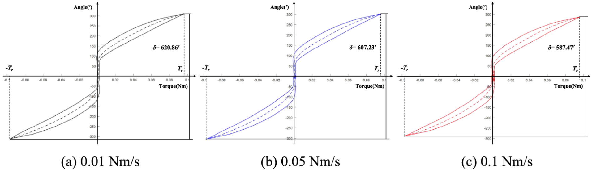
Hysteresis curves of Reducer 2: (a) 0.01 Nm/s, (b) 0.05 Nm/s, and (c) 0.1 Nm/s.

Analysis shows: (1) The hysteresis curve of Reducer 1 is an inverted Z-shape. The area enclosed near the 0 Nm position is large, while the area enclosed away from the 0 Nm position is small, appearing wide in the middle and narrow at both ends, reflecting the reducer’s large geometric backlash. Furthermore, as the loading rate increases, the change in the output rotation angle value at the peak point is small, indicating little influence from the loading rate. (2) The hysteresis curve of Reducer 2 is S-shaped. The area enclosed near the 0 Nm position is small, while the area enclosed away from the 0 Nm position is large, appearing narrow in the middle and wide at both ends, reflecting small geometric error and large elastic deformation. As the loading rate increases, the output rotation angle value at the peak point shows a decreasing trend, decreasing by about 5′ each time. (3) Under the same loading rate, the output rotation angle at the peak point of Reducer 1 is smaller than that of Reducer 2, indicating that material affects the backdrivability of the reducer.

Variation patterns of S and u

The variation of S for Reducers 1 and 2 is shown in Figure 15. In the figure, the area change of the hysteresis curve for Reducer 1 is relatively stable, reflecting that the dissipated energy of Reducer 1 is in a relatively stable state. Comparing with Figure 13, it indicates that Reducer 1 itself consumes more energy due to geometric errors. The change in S for Reducer 1 under different loading rates is not significant, indicating that the loading rate has little effect on the energy dissipation of the metal gear reducer, meaning its backdrivability is insensitive to impact conditions.

Figure 15.

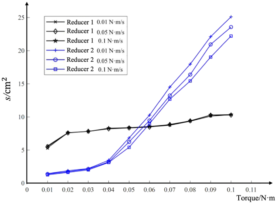
Variation of S under different loading rates.

The area of the hysteresis curve for Reducer 2 increases nearly linearly with the increase in torque, and energy consumption rises rapidly. Corresponding to Figure 14, this reflects less energy consumed by geometric errors and more energy consumed by friction. The change in S for Reducer 2 under different loading rates shows differences. When the torque is less than 0.04 Nm, the three curves are relatively close. When the torque exceeds 0.04 Nm, the three curves diverge, showing different S changes. It was found that the smaller the loading rate, the larger the S. These results indicate that the loading rate affects the energy dissipation capacity of Reducer 2, meaning the back-driving capability of Reducer 2 is influenced by load fluctuations.

The reason for the different energy consumption during reverse rotation between Reducers 1 and 2 is: the plastic gears have lower stiffness and are prone to deformation. The change in gear system dynamics is inconsistent with the loading rate. The faster the loading rate, the less sufficient the frictional energy consumption.

The variation of the energy dissipation ratio u for Reducers 1 and 2 when loaded to different torque positions is shown in Figure 16. In the figure, as the output torque increases incrementally, the total absorbed strain energy of Reducer 1 increases rapidly, but the energy dissipation ratio decreases rapidly, with the highest energy dissipation rate at 0.01 Nm. From Figures 13 and 16, the dissipated energy remains relatively stable, indicating low energy utilization efficiency of the reducer. As torque increases, the hysteresis curve shape becomes slender. The change in u for Reducer 1 under different loading rates is small, indicating that the loading rate has little effect on it, once again verifying that the backdrivability of Reducer 1 has no strong correlation with external load fluctuations.

Figure 16.

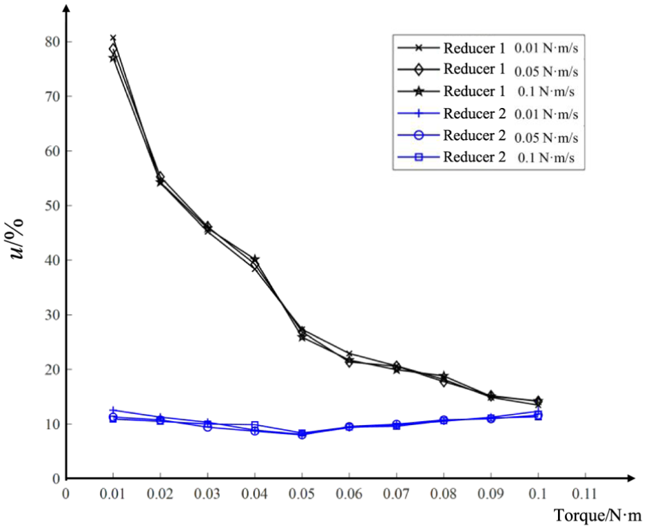
Variation of u under different loading rates.

The variation pattern of energy dissipation for Reducer 2 is different from that of Reducer 1. In Figure 16, as the output torque increases incrementally, the energy dissipation ratio first decreases and then increases, remaining at a relatively low overall level, reaching the lowest point at 0.05 Nm. As known from Figure 15, as torque increases, the hysteresis curve area S gradually increases, and dissipated energy gradually increases, but the total absorbed strain energy increases faster, causing the energy dissipation ratio to gradually decrease. Upon reaching 0.05 Nm, the dissipated energy begins to increase rapidly, at a speed higher than the increase speed of the total absorbed strain energy. At this point, the energy dissipation ratio begins to increase. The shape of the hysteresis curve shows a change process of “slender–wide and thick–slender.” Similarly, the influence of the loading rate is small.

Torque-energy variation analysis

The torque-energy curves of Reducers 1 and 2 under loading rates of 0.01, 0.05, and 0.1 Nm/s are shown in Figure 17. The torque-energy curves of both reducers are double-hump curves, but there are obvious differences between them. The ranges of the W_m1 and W_m2 regions for the metal reducer are much smaller than the W_p1 and W_p2 regions for the plastic reducer, while the W_m3 region is much larger than the W_p3 region.

Figure 17.

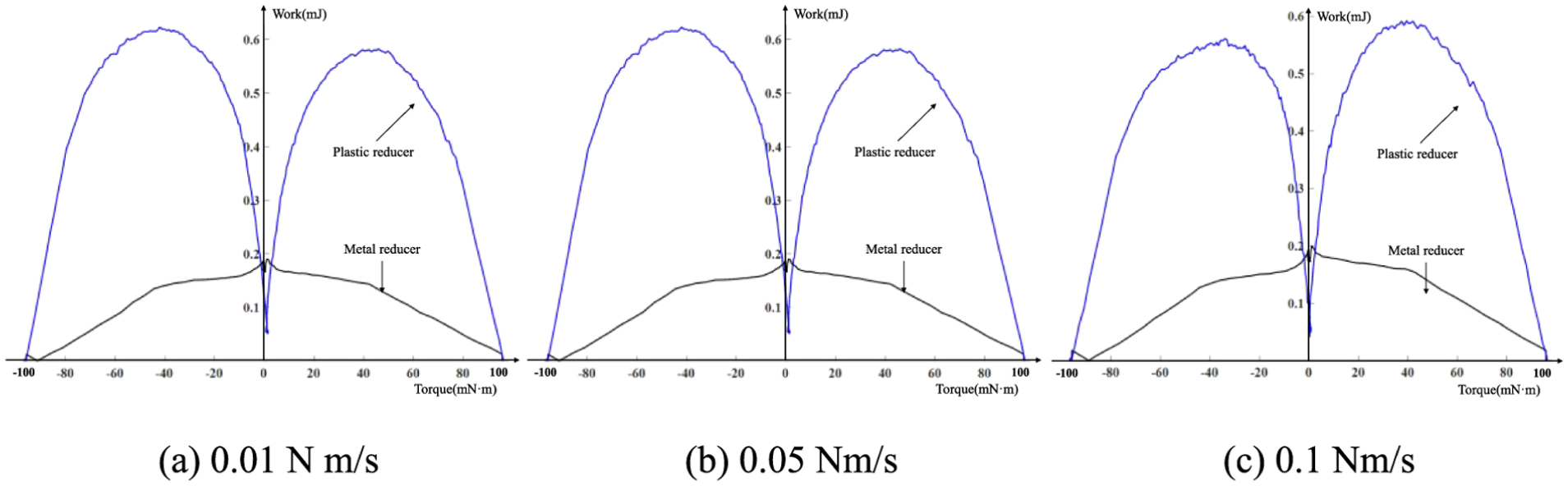
Torque-energy curves of Reducer 1 and Reducer 2: (a) 0.01 N m/s, (b) 0.05 Nm/s, and (c) 0.1 Nm/s.

The W_m1 and W_m2 regions of the metal gear reducer are within the range of [−0.01 Nm, 0.01 Nm]. This range is mainly influenced by geometric errors, with less influence from elastic deformation. Within this region, the energy absorption generated by the reducer’s reversal reaches its highest point, meaning the area enclosed in the hysteresis curve is the largest. This reflects that geometric error is the main factor affecting the energy consumption of the powder metallurgy reducer. The W_p1 and a small part of the W_p2 regions of the plastic gear reducer are within the range of [−0.01 Nm, 0.01 Nm]. Within this range, energy consumption does not reach the highest point, meaning the area enclosed in the hysteresis curve is the smallest. This range is mainly influenced by elastic deformation, with less influence from geometric errors, reflecting that elastic deformation is the main part absorbing energy.

Overall, the mechanisms by which the two reducers release energy during back drive are fundamentally different. Reducer 1 primarily absorbs impact energy through geometric error factors, while Reducer 2 absorbs impact energy through elastic deformation. The core factors causing this difference are tolerance fit and material stiffness. This conclusion prompts us to consider: if pursuing ultimate backdrivability, then having a certain geometric backlash and gears with certain flexibility is beneficial, but such a design will consume more energy, thereby reducing the efficiency and precision characteristics of the reducer. Therefore, for a given reduction ratio, backdrivability involves finding a balance between stiffness, geometric backlash, and reducer performance.

Value and application

This paper provides means for studying the backdrivability of reducers. For the design research of reducer backdrivability, within the comprehensive performance range of the reducer in its usage scenario, the optimal combination of geometric backlash and structural stiffness should be sought. The hysteresis curve can be used for lost motion design, controlling the rotation angle by controlling the value of the lost motion. Using the area S enclosed by the hysteresis curve as the target, controlling the area of the hysteresis curve enables control over the reducer’s energy absorption, thus meeting the design requirements for backdrivability under different working environments. The testing of reducer backdrivability is even more significant. By simply testing the reducer’s hysteresis curve and analyzing the lost motion, area S, and energy dissipation ratio u, a more comprehensive understanding of the reducer’s backdrivability can be achieved.

Moreover, in practical applications, backlash and return clearance can degrade both the dynamic response speed and positioning accuracy of the reducer. These effects can be mitigated during design and manufacturing through several strategies: tightening tolerances on component machining; establishing rational precision allocation guidelines; selecting materials with low coefficients of thermal expansion; enhancing gear manufacturing accuracy; and improving assembly consistency. Additionally, system-level compensation techniques—such as implementing gap-compensation algorithms in the control software or adopting dual-motor differential drive schemes—can actively suppress nonlinear torque fluctuations induced by mechanical backlash. By adopting these methods, transmission accuracy can be ensured while simultaneously improving the reducer’s energy absorption capacity under sudden loads and its reverse-drive response speed.

Conclusion

Through theoretical analysis and experiments, this paper studied the backdrivability of reducers and obtained the following conclusions:

(1) The essence of back drive is the reverse impact of load torque fluctuation on the reducer. It is defined as the ability to quickly reverse and absorb external energy when the load torque at the output end of the reducer changes abruptly;

(2) When the reducer load changes, the hysteresis characteristics of the reducer can be utilized to reflect its backdrivability through the rotation angle and energy absorption;

(3) Lost motion can reflect the rotation angle of the reducer, and the area enclosed by the hysteresis curve can reflect the energy absorption capacity of the reducer;

(4) The backdrivability of the reducer is directly related to its geometric backlash and system stiffness. Under the premise that the reducer’s performance meets the usage scenario, increasing geometric backlash and reducing system stiffness are more beneficial for backdrivability;

(5) The analytical method proposed in this paper exhibits high applicability and is suitable for both conceptual design-stage operating conditions and actual operational conditions of reducers in complex application scenarios. Future research will focus on situations with more complex nonlinear load changes to more realistically simulate the back-driving scenarios of robots in actual operations.

Footnotes

Appendix

All the characters cited in this article and their corresponding explanations are shown in Table 1.

ORCID iD

Da Cao

Ethical considerations

This article does not include any studies on human participants conducted by the author.

Consent to participate

This article does not involve any biological research.

Consent for publication

This manuscript has not been published or presented elsewhere in part or in entirety, and is not under consideration by another journal. All the authors have approved the manuscript and agree with submission to your esteemed journal.

Author contributions

This study was jointly completed by five researchers, among whom Da Cao is the first author and Huiming Cheng is the corresponding author (chenghuiming295@126.com). The contributions of each author to this paper are as follows: Da Cao (First Author): Conceptualization, Methodology, Formal Analysis, Writing - Review & Editing; Huiming Cheng (Corresponding Author): Investigation, Data Curation; Zhaoyao Shi: Supervision, Writing - Review & Editing. This manuscript is our original work and has not been published nor is it currently under consideration for publication elsewhere. All authors have approved the contents of this paper and have agreed to the submission policy of Mechatronics.

Funding

The authors disclosed receipt of the following financial support for the research, authorship, and/or publication of this article: This work was supported by The National Key Research and Development Program of China (Grant No. 2024YFB3410404).

Declaration of conflicting interests

The authors declared no potential conflicts of interest with respect to the research, authorship, and/or publication of this article.

Data availability statement

The raw/processed data required to reproduce the above findings cannot be shared at this time as the data also forms part of an ongoing study.

References

Kang

Peterson

Herrin

, et al. Design and validation of a torque-controllable series elastic actuator-based hip exoskeleton for dynamic locomotion. J Mech Robot 2023; 15(2): 021007.

Lee

Joo

Kang

, et al. A review on the force sensing and force feedback-based navigation of mobile robots. Int J Precis Eng Manuf 2025; 26: 1291–1311.

Garcia

Saerens

Crispel

, et al. Factors influencing actuator’s backdrivability in human-centered robotics. MATEC Web Conf 2022; 366: 01002.

, et al. Wearable extra robotic limbs: a systematic review of current progress and future prospects. J Intell Robot Syst 2023; 109(1): 16.

Nabeshima

Ayusawa

Hochberg

, et al. Standard performance test of wearable robots for lumbar support. IEEE Robot Autom Lett 2018; 3(3): 2182–2189.

Zhu

Jiao

Dominguez

, et al. Design and backdrivability modeling of a portable high torque robotic knee prosthesis with intrinsic compliance for agile activities. IEEE/ASME Trans Mechatron 2022; 27(4): 1837–1845.

Heo

Kim

. Backdrivable and fully-portable pneumatic back support exoskeleton for lifting assistance. IEEE Robot Autom Lett 2020; 5(2): 2047–2053.

Laliberté

Abdallah

Gosselin

. A backdrivable 6-dof parallel robot for sensorless dynamically interactive tasks. Robot Comput Integr Manuf 2024; 86: 102642.

Yokoyama

Shimono

. Back-drivability improvement of geared system based on disturbance observer and load-side disturbance observer. IEEJ J Ind Appl 2020; 9(5): 475–485.

10.

Kaminaga

Amari

Katayama

, et al. Backdrivability analysis of electro-hydrostatic actuator and series dissipative actuation model. In: 2010 IEEE international conference on robotics and automation, 2010, pp.4204–4211.

11.

Nef

Lum

. Improving backdrivability in geared rehabilitation robots. Med Biol Eng Comput 2009; 47(4): 441–447.

12.

Calanca

Muradore

Fiorini

. A review of algorithms for compliant control of stiff and fixed-compliance robots. IEEE/ASME Trans Mechatron 2016; 21(2): 613–624.

13.

Shah

Doss

ASA

Lakshmaiya

. Advancements in AI-enhanced collaborative robotics: towards safer, smarter, and human-centric industrial automation. Results Eng 2025; 27: 105704.

14.

Kumar

Savur

Sahin

. Survey of human–robot collaboration in industrial settings: awareness, intelligence, and compliance. IEEE Trans Syst Man Cybern Syst 2021; 51(1): 280–297.

15.

De Maddis

Razza

Basile

, et al. Robot-assisted quasi-simultaneous laser welding of thermoplastics. Int J Adv Manuf Technol 2025; 138: 2031–2042.

16.

Liu

Zhang

, et al. Accurate impedance control for robot joints with 3K gear reducers based on transmission efficiency. In: 2025 IEEE 20th conference on industrial electronics and applications (ICIEA), 2025.

17.

Shan

Endo

Tsutsui

, et al. Improving back-drivability of robot joint by reducing reflected inertia using multi-motor system. In: 2025 IEEE/SICE international symposium on system integration (SII), 2025, pp.414–421.

18.

Zinn

Khatib

Roth

, et al. Playing it safe: human-friendly robots. IEEE Robot Autom Mag 2004; 11(2): 12–21.

19.

Shin

Ahn

Kwon

. A low backlash and highly efficient gearbox for robot actuator. In: 2024 IEEE International Conference on Advanced Intelligent Mechatronics (AIM), 2024

20.

Ishida

Takanishi

. A robot actuator development with high backdrivability. In: 2006 IEEE conference on robotics, automation and mechatronics, 2006, pp.1–6.

21.

van Meer

van Meijel

van Halsema

, et al. Compensating hysteresis and mechanical misalignment in piezo-stepper actuators. Mechatronics 2025; 111: 2503.

22.

Bisquert

. Hysteresis, impedance, and transients effects in halide perovskite solar cells and memory devices analysis by neuron-style models. Adv Energy Mater 2024; 14(26): 2400442.

23.

Wang

Chen

. Experimental study on the influence of flexible bearing clearance on natural frequency of harmonic reducer. J Adv Mech Des Syst Manuf 2022; 16(1): JAMDSM0012.

24.

Terada

Makino

Wada

, et al. Improved design of an orthogonal-axis-type precession motion ball reducer. J Mech Robot 2024; 16(9): 091010.

25.

Shi

, et al. Dynamic measurement of the lost motion of precision reducers in robots and the determination of optimal measurement speed. J Adv Mech Des Syst Manuf 2019; 13(3): JAMDSM0044.

26.

Shi

Yang

, et al. Hysteresis curve model of precision reducers in robots and its application in lost motion evaluation. Meas Sens 2025; 38: 101848.

Research on back driving performance of robot reducers based on hysteresis characteristics