Sage Journals: Discover world-class research

Abstract

DC–DC buck converters are inherently nonlinear systems that often operate under dynamically changing conditions, parameter uncertainties, and external disturbances, posing significant challenges for conventional control strategies. This paper introduces a novel cascaded proportional–integral and proportional–derivative (PI–PD) controller architecture, in which all controller parameters are optimally tuned using the recently developed Electric Eel Foraging Optimizer (EEFO), a bio-inspired metaheuristic algorithm modeled on the electrolocation and hunting behaviors of electric eels. The proposed control structure uniquely integrates a dual-loop configuration: the inner PI loop eliminates steady-state error, while the outer PD loop enhances dynamic response and mitigates rapid transient fluctuations. This cascaded arrangement enables decoupled tuning of steady-state and transient characteristics, offering superior control flexibility compared to conventional single-loop PID designs. To calibrate the controller, EEFO is employed to minimize a composite performance objective function that simultaneously considers settling time and overshoot, ensuring well-damped and rapid system behavior. A comprehensive set of simulation experiments was conducted in a MATLAB/Simulink environment to evaluate the proposed method against multiple benchmark algorithms—including the flood algorithm, gazelle optimization algorithm, and artificial hummingbird algorithm—as well as classical PID, PID acceleration (PIDA), and fractional-order PID (FOPID) controllers optimized by state-of-the-art metaheuristics. Across all key performance metrics—including rise time, settling time, percentage overshoot, peak time, and steady-state error—the EEFO-tuned cascaded PI–PD controller demonstrated consistently superior results, achieving near-zero overshoot, ultra-fast convergence, and minimal output deviation. Beyond nominal conditions, extensive robustness analyses were conducted to validate the controller’s effectiveness under realistic disturbances, such as abrupt load changes, high-frequency measurement noise, time-delay effects in feedback channels, and ±10%–15% parametric variations in inductance and capacitance. In all scenarios, the controller retained stable output regulation, confirming its resilience and practical viability. To the best of our knowledge, this is the first study to deploy a cascaded PI–PD control structure specifically designed for DC–DC buck converters and optimized using the EEFO algorithm. The integration of a biologically inspired optimization framework with a decoupled dual-loop control scheme offers both architectural and algorithmic novelty. The proposed strategy addresses critical demands in nonlinear converter regulation and provides a robust, high-performance solution suitable for dynamic and uncertain power electronic environments.

Keywords

artificial intelligence bio-inspired algorithms buck converter cascaded PI–PD controller DC–DC power conversion EEFO algorithm metaheuristic control nonlinear dynamical systems robust regulation uncertainty modeling

Introduction

Numerous systems employed in contemporary technology, including computers, electrical appliances, power supply, motor drivers, green hydrogen and solar energy systems, require diverse voltage levels. Various converters, such as buck, boost and buck-boost enable the attainment of requisite voltage levels in designated systems and devices. Buck converters, known for their optimal efficiency and minimal loss of energy during conversion, are widely utilized. Buck converters present a robust solution in several technological applications because to their modular design, cost-effectiveness, and exceptional performance.¹

Developing a suitable model for stable and high-efficiency systems is very important in buck converters. Their nonlinear nature poses a challenge in developing a stable control system. Buck converters, widely used for generating various output voltages based on a specified input voltage, exhibit significant sensitivity to reference alterations, prompting considerable interest from researchers in this area.² In response to issues such as abrupt load variations and the generation of undulating output voltages during switching operations, numerous research has been conducted focused on the design of low-loss, high-efficiency linear controller systems and the optimization of parameters.

In recent years, metaheuristic optimization techniques^3–8 have shown remarkable promise in improving the dynamic performance of DC–DC converters. Several studies have optimized PID controllers using approaches such as the improved sine cosine algorithm (ISCA),⁹ golden eagle optimization (GEO),¹⁰ genetic algorithm,¹¹ Harris hawks optimization,¹² artificial hummingbird algorithm,¹³ and hunger games search algorithm,¹⁴ all demonstrating superior adaptability to complex control problems. For example, Nanyan et al.⁹ effectively utilized ISCA to achieve improved convergence characteristics while avoiding local optima, a common issue in traditional techniques.

Additionally, more sophisticated control frameworks^15–17 have emerged to address nonlinear converter dynamics. Warrier et al.¹⁸ proposed a complex-order PI controller tuned via a cohort intelligence algorithm, while Demircan et al.¹⁹ compared PD, PI, and PID controllers optimized via the artificial bee colony algorithm and concluded that PID structures yielded the most balanced trade-off between speed and accuracy.

Expanding upon these earlier efforts, Ersali et al.²⁰ employed a hybrid adversarial snake optimization and pattern search method to tune a cascaded first-order filtered PID controller, using opposition-based learning to enhance exploration–exploitation balance. Similarly, Izci et al.²¹ combined artificial ecosystem optimization with the Nelder–Mead method to improve PID tuning outcomes. Hybrid methods such as improved golden jackal optimization,²² dandelion optimizer,²³ and prairie dog optimization–marine predator algorithm²⁴ further underscore the growing trend of using biologically inspired computation to refine control strategies.

Complementing these advancements, the role of intelligent and adaptive control systems has been emphasized. For instance, Saleem et al.²⁵ proposed a fuzzy-augmented model reference adaptive PID control structure (FMRAC–PID), achieving enhanced robustness under nonlinear and time-varying operating conditions.

In parallel, several recent studies have explored the design and real-time application of PI–PD and I–PD controllers, particularly for challenging industrial process models involving instability, dead-time, and inverse response characteristics. For example, robust PI–PD strategies have been proposed for unstable and integrating chemical processes using predictive²⁶ and enhanced two-degree-of-freedom designs,²⁷ while Smith predictor-based PI–PD schemes have proven effective for plants with significant delays.²⁸ Furthermore, I–PD structures have demonstrated improved loop decoupling and steady-state performance in complex industrial setups such as boiler steam drums and bioreactors,²⁹ as well as in cases involving inverse responses and open-loop zeros.³⁰

It is important to emphasize that, although PI–PD and I–PD control structures have been widely studied in industrial process control and chemical engineering applications (particularly for unstable, integrating, inverse-response, and dead-time-dominant systems^26–30) their adoption in DC–DC buck converter control has remained largely unexplored. A thorough review of the existing buck-converter literature reveals that most studies continue to rely on classical PID, PID acceleration, or fractional-order PID controllers, with research efforts primarily directed toward improving parameter tuning through advanced optimization techniques rather than revisiting the underlying control architecture. One plausible reason for this gap is the long-standing dominance of single-loop PID paradigms in power electronics, where fast electrical dynamics and switching behavior have traditionally favored simpler control structures. Consequently, the potential benefits of cascaded PI–PD configurations (particularly their ability to decouple transient shaping from steady-state regulation) have not been systematically investigated for buck converter applications. The present study addresses this gap by adapting a cascaded PI–PD structure to the specific dynamic characteristics of DC–DC buck converters and rigorously evaluating its performance and robustness under nonlinear and uncertain operating conditions. Drawing inspiration from such works, this study explores a cascaded PI–PD controller framework optimized using the electric eel foraging optimizer (EEFO).³¹

The primary motivation behind this design is to merge the complementary strengths of PI and PD actions: the integral term in PI eliminates steady-state errors, while the derivative term in PD suppresses abrupt transient responses. The novelty lies in two dimensions: it is the first to deploy a PI–PD structure in a DC–DC buck converter application and the first to utilize the biologically inspired EEFO algorithm for gain tuning. EEFO, modeled after the electro-sensory foraging behavior of electric eels, offers a highly effective search mechanism capable of exploring and exploiting the control parameter space for rapid convergence and robust outcomes.

To validate this design, we perform an extensive set of comparative analyses against both well-established and emerging optimization methods, including flood algorithm, gazelle optimization algorithm, and artificial hummingbird algorithm, as well as reported PID, PID acceleration (PIDA), and fractional-order PID (FOPID) controllers optimized by various metaheuristics. The obtained results consistently show that our EEFO-based PI-PD controller not only converges more rapidly to high-quality solutions (as evidenced by objective function metrics) but also achieves faster settling, zero overshoot, and lower error-based measures than competing methods. Furthermore, we examine its performance under practical disturbances, such as measurement noise, abrupt load changes, time delays, and parameter uncertainties in circuit components. In all cases, the proposed controller retains stable regulation with negligible overshoot and minimal steady-state deviation. Unlike prior studies that typically apply classical PID or fractional controllers optimized by standard algorithms, this study is the first to integrate a cascaded PI-PD controller with the recently introduced EEFO. This hybridization provides both architectural and algorithmic novelty in addressing the robust control needs of nonlinear buck converter systems. Accordingly, the novelty of this study is established along two clearly distinguished dimensions:

Control-structure contribution: the first application of a cascaded PI–PD controller for DC–DC buck converter regulation, enabling explicit decoupling of transient and steady-state control objectives.

Optimization-algorithm contribution: the first use of the EEFO algorithm for tuning PI–PD controller parameters in power electronic converter control.

The proposed EEFO-based PI–PD controller is evaluated through extensive simulations and fair comparisons with state-of-the-art optimization techniques and reported PID, PIDA, and FOPID controllers. Robustness is further assessed under realistic non-ideal operating conditions, including load disturbances, measurement noise, time delays, and parameter uncertainties. The results demonstrate that the proposed approach achieves superior dynamic response, negligible overshoot, and high steady-state accuracy while maintaining robust performance across a wide range of operating scenarios.

The remainder of this paper is organized as follows. Section 2 presents the mathematical modeling of the buck converter. Section 3 describes the Electric Eel Foraging Optimizer. Section 4 introduces the proposed EEFO-based cascaded PI–PD controller. Section 5 discusses comparative simulation results, while Section 6 evaluates robustness under non-ideal conditions. Finally, Section 7 concludes the paper and outlines future research directions.

Mathematical modeling of DC-DC buck converter

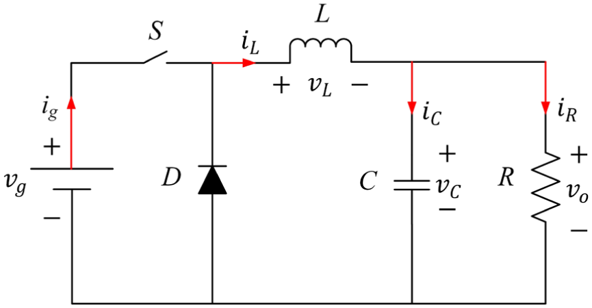
The working principle of buck converters, which are used to obtain a low DC voltage for a high DC voltage, is usually based on the integration of a series switching and inductor and energy storage processes controlled by a metal oxide semiconductor field-effect transistor (MOSFET). As a result of the on-off operation of switching elements such as MOSFET or insulated-gate bipolar transistor (IGBT), continuously increasing or decreasing inductor currents may occur, as well as fluctuating output voltages. These conditions, which occur in current or voltage over time, make DC-DC Buck converter systems nonlinear. As shown in Figure 1, the DC-DC Buck converter circuit basically consists of a DC fed source, a switching mechanism controlled by a method called pulse width modulation, diode, inductor and capacitor filters and a load fed by the circuit.¹⁰ In this structure, V_g symbolizes the source voltage, D is the duty cycle, L is the inductor, C is the capacitor, R is the load resistance.

Figure 1.

Mathematical model of uncontrolled buck converter system.

In a complete switching period, with period T_s, T_on symbolizes the time when switch S is closed and T_off symbolizes the time when it is open. In the control loop, the duty cycle (D), defined as the ratio of the switch-on time (T_on) to the total switching period (T_s), plays a key role in regulating the output voltage. The relationship between D, T_on and T_off is expressed by equations (1) and (2).¹⁰

T_{on} = D T_{s}

(1)

T_{off} = (1 - D) T_{S}

(2)

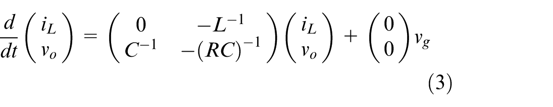
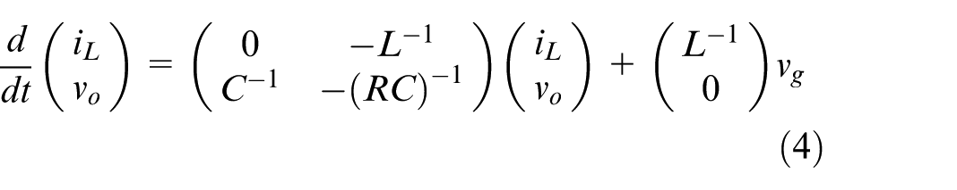
The equations of state based on Kirchoff’s law for the open and closed positions of switch S are expressed by open mode (switch off) and close mode (switch on) which are given in equations (3) and (4), respectively.¹⁰

\frac{d}{dt} (\begin{matrix} i_{L} \\ v_{o} \end{matrix}) = (\begin{matrix} 0 & - L^{- 1} \\ C^{- 1} & - {(RC)}^{- 1} \end{matrix}) (\begin{matrix} i_{L} \\ v_{o} \end{matrix}) + (\begin{matrix} 0 \\ 0 \end{matrix}) v_{g}

(3)

\frac{d}{dt} (\begin{matrix} i_{L} \\ v_{o} \end{matrix}) = (\begin{matrix} 0 & - L^{- 1} \\ C^{- 1} & - {(RC)}^{- 1} \end{matrix}) (\begin{matrix} i_{L} \\ v_{o} \end{matrix}) + (\begin{matrix} L^{- 1} \\ 0 \end{matrix}) v_{g}

(4)

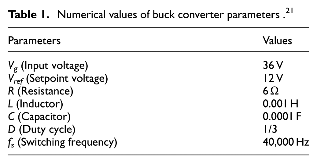
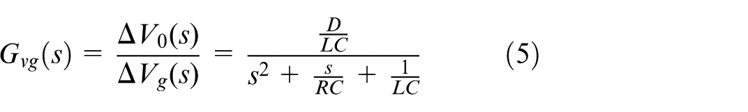
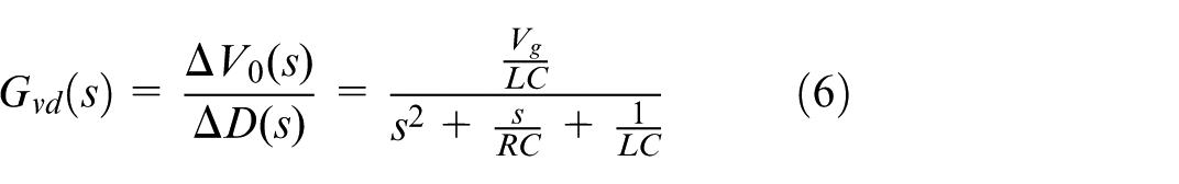
The small signal (dynamic) model of the DC-DC converter circuit given in Figure 2, which shows the transfer function between control and output, is given in Figure 2.³² The parameters used in the DC-DC converter simulation circuit considered in this study are shown in Table 1.²¹ Here reference voltage is taken as 12 V, source voltage as 36 V, load resistance as 6 Ω, filter inductor as 1 mH, filter capacitor as 100 µF, duty cycle as 1/3 and switching frequency as 40 kHz.³³ With the Mason gain formula in this model, the small-signal transfer functions of the DC-DC step-down converter can be obtained.³⁴ Equation (5) is the small-signal transfer function from input to output with the capacitor voltage as the output voltage reference, while equation (6) expresses the small-signal transfer function from control to output with the capacitor voltage as the output voltage reference.

Figure 2.

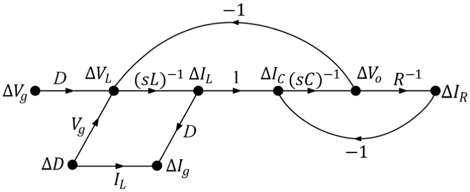
Small signal model of buck converter system.

Table 1.

Numerical values of buck converter parameters .²¹

Parameters	Values
V _g (Input voltage)	36 V
V _ref (Setpoint voltage)	12 V
R (Resistance)	6 Ω
L (Inductor)	0.001 H
C (Capacitor)	0.0001 F
D (Duty cycle)	1/3
f _s (Switching frequency)	40,000 Hz

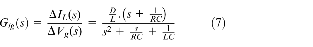
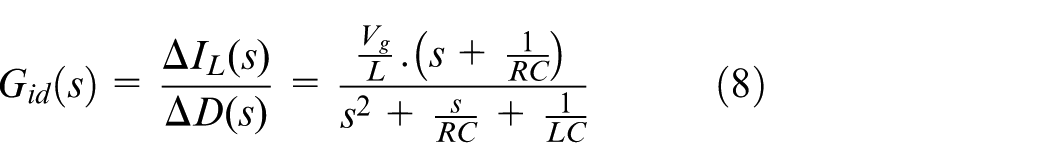
In equations (7) and (8), the inductor current is selected as the output and the input-to-output and control-to-output small-signal transfer function are expressed with reference to this current.³⁴

G_{vg} (s) = \frac{Δ V_{0} (s)}{Δ V_{g} (s)} = \frac{\frac{D}{LC}}{s^{2} + \frac{s}{RC} + \frac{1}{LC}}

(5)

G_{vd} (s) = \frac{Δ V_{0} (s)}{Δ D (s)} = \frac{\frac{V_{g}}{LC}}{s^{2} + \frac{s}{RC} + \frac{1}{LC}}

(6)

G_{ig} (s) = \frac{Δ I_{L} (s)}{Δ V_{g} (s)} = \frac{\frac{D}{L} . (s + \frac{1}{RC})}{s^{2} + \frac{s}{RC} + \frac{1}{LC}}

(7)

G_{id} (s) = \frac{Δ I_{L} (s)}{Δ D (s)} = \frac{\frac{V_{g}}{L} . (s + \frac{1}{RC})}{s^{2} + \frac{s}{RC} + \frac{1}{LC}}

(8)

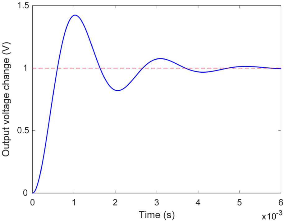
The open loop response of the Buck converter system is shown in Figure 3. As can be seen, there is a high overshoot in the response to a step change of $δ d = 1 / 36$ and a long settling time is observed.¹⁰ The nonlinear structures of these systems, in which high efficiency is achieved with near-minimum power losses despite high power transfers, as mentioned above, necessitate the design of the most suitable controller for DC-DC Buck converter circuits.

Figure 3.

Open-loop step response of buck converter.

Although the DC–DC buck converter is inherently nonlinear due to its switching behavior and duty-cycle-dependent dynamics, a small-signal averaged model is adopted in this study to facilitate controller design and comparative evaluation. The linearization is performed around a nominal steady-state operating point defined by the rated input voltage, duty cycle, load resistance, and passive component values listed in Table 1. This operating point corresponds to normal regulation conditions, where the converter is expected to maintain stable output voltage with small perturbations around the reference. The resulting small-signal model accurately captures the local dynamic behavior of the system and is widely used in control-oriented analysis of power electronic converters. It is acknowledged that the validity of this linearized representation may degrade under large-signal excursions or strongly nonlinear operating conditions. For this reason, the controller’s performance is further validated through extensive nonlinear time-domain simulations under realistic disturbances, uncertainties, and delays, as presented in the last section of this paper, thereby ensuring robust operation beyond the assumptions of the small-signal model.

Overview of electric eel foraging optimizer

Electric eels, whose habitat is freshwater in the Amazon region of South America, have inspired the EEFO method with their fishing methods in order to survive. Due to their poor eyesight, these fish use $10 V$ electrical signals to locate their prey.³⁵ Electric eels, which locate their prey with the responses from these signals, stun their prey with a voltage of around $600 - 800 V$ they produce this time. The low and high voltages they use to locate and hunt their prey are generated by the hundreds of electrocytes they contain.³⁶ The mathematical model and algorithm of EEFO, which is inspired by their behavior in both interaction and hunting processes, are described below.

Although the EEFO is presented here in its general form, its internal mechanisms are directly aligned with the requirements of the cascaded controller (given in the next section) tuning problem addressed in this study. In particular, the interaction and migration phases facilitate broad exploration of the multidimensional controller gain space, which is essential for avoiding premature convergence when simultaneously tuning proportional, integral, and derivative parameters. The resting behavior supports stabilization around promising gain combinations, while the hunting phase enables refined local exploitation once desirable transient and steady-state characteristics are identified. Moreover, the adaptive transition between exploration and exploitation governed by the energy factor allows EEFO to balance fast convergence with solution robustness. These properties make EEFO especially suitable for optimizing the cascaded structure, where strong coupling between controller gains and nonlinear system dynamics necessitates a search strategy capable of both global diversity and precise local refinement.

Interaction

Each eel in a school of electric eels, which exhibit mass-living behavior by swimming and turning together, represents a candidate solution. When they encounter a school of fish, they cooperate with the other eels in the school to try to gather their target school of fish in the center of the surrounding area.³⁷ The interaction phase of the EEFO algorithm is the comparison of the location of each of these fish with the location information of other fish in their shoal. These movements that occur during the interaction phase are referred to as “churn” and these random movements are given in equation (9).³¹ In this expression, $n_{1} ~ N (0, 1)$ and $B = [b_{1}, b_{2}, b_{3}, \dots, b_{k}, \dots, b_{d}]$ .

C = n_{1} x B

(9)

The interaction phase in the EEFO algorithm is shown as follows.

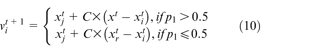
v_{i}^{t + 1} = {\begin{matrix} x_{j}^{t} + C \times (x^{t} - x_{i}^{t}), if p_{1} > 0.5 \\ x_{j}^{t} + C \times (x_{r}^{t} - x_{i}^{t}), if p_{1} \leq 0.5 \end{matrix}

(10)

In equation (10), $p_{1} ve p_{2}$ are randomly selected numbers between 0 and 1, and x_r is the sum of the difference between the upper and lower bounds multiplied by a randomly chosen number (r). In a population of size n, x(t) is expressed as in equation (11).

x (t) = \frac{1}{n} \sum_{i = 1}^{n} x_{i}^{t}

(11)

Resting

The resting behavior of the EEFO algorithm starts with determining a resting area where any of the available position vectors of the eels is selected on the main diagonal of the search region. As with the interaction behavior of eels, the resting phase after feeding should also be represented in the EEFO. To do this, a resting area is created for the eel, where any of the dimensions of its position vector are positioned on the diagonals of the search space, and then the eels move toward this resting area. The rest phase in the EEFO algorithm is expressed by equation (12).³⁸

v_{i}^{t + 1} = R_{i}^{t + 1} + n_{2} \times (R_{i}^{t + 1} round (rand) \times x_{i}^{t})

(12)

In equation (12), R_i is resting position and $n_{2} (0, 1)$

Hunting

By interacting with other members of their schools, eels surround the school of fish they target as prey and use low-voltage stresses to drag them from deeper waters to shallower waters where they can hunt them more easily.³⁷ The fish in the targeted shoal exhibit serial displacement movements due to panic in this circular area, which is referred to as the hunting area. The wriggling reactions of eels during fishing behavior are expressed in equation (13).³⁸

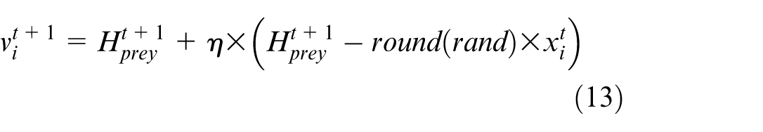
v_{i}^{t + 1} = H_{prey}^{t + 1} + η \times (H_{prey}^{t + 1} - round (rand) \times x_{i}^{t})

(13)

In this equation, the position of the prey in the hunting zone is symbolized by H_prey and the curl factor is symbolized by η.

Migration

When resting eels detect prey, they tend to show migratory behavior from the resting area to the hunting area.³⁷ This migration behavior is expressed in equation (14).³¹

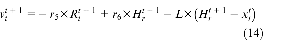
v_{i}^{t + 1} = - r_{5} \times R_{i}^{t + 1} + r_{6} \times H_{r}^{t + 1} - L \times (H_{r}^{t + 1} - x_{i}^{t})

(14)

In this equation, any point H_r, at the capture point is represented by the Levy flight function L, and r₅, r₆ are randomly selected values between 0 and 1.

Transition from exploration to exploitation

For a high optimization performance in the EEFO algorithm, the transition from the exploration phase to the exploitation phase needs to be managed efficiently. For this efficient management an energy factor value is used, expressed by equation (15).³⁶

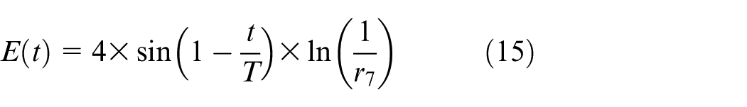
E (t) = 4 \times \sin (1 - \frac{t}{T}) \times \ln (\frac{1}{r_{7}})

(15)

In this equation, r₇ is a randomly chosen value between 0 and 1. The working principle of the EEFO algorithm is given in Figure 4. The process starts with the definition of the algorithm parameters and continues with the definition of an initial population of random individuals whose solution space each represents a potential solution. In this randomized process to avoid local minimization, a fitness value is defined for each solution, representing the fitness of the solution to the targeted problem. Here, four different behaviors such as interacting, resting, migrating and hunting are used to achieve the best results in scanning the solution space. This algorithm stops when the maximum number of iterations is reached.

Figure 4.

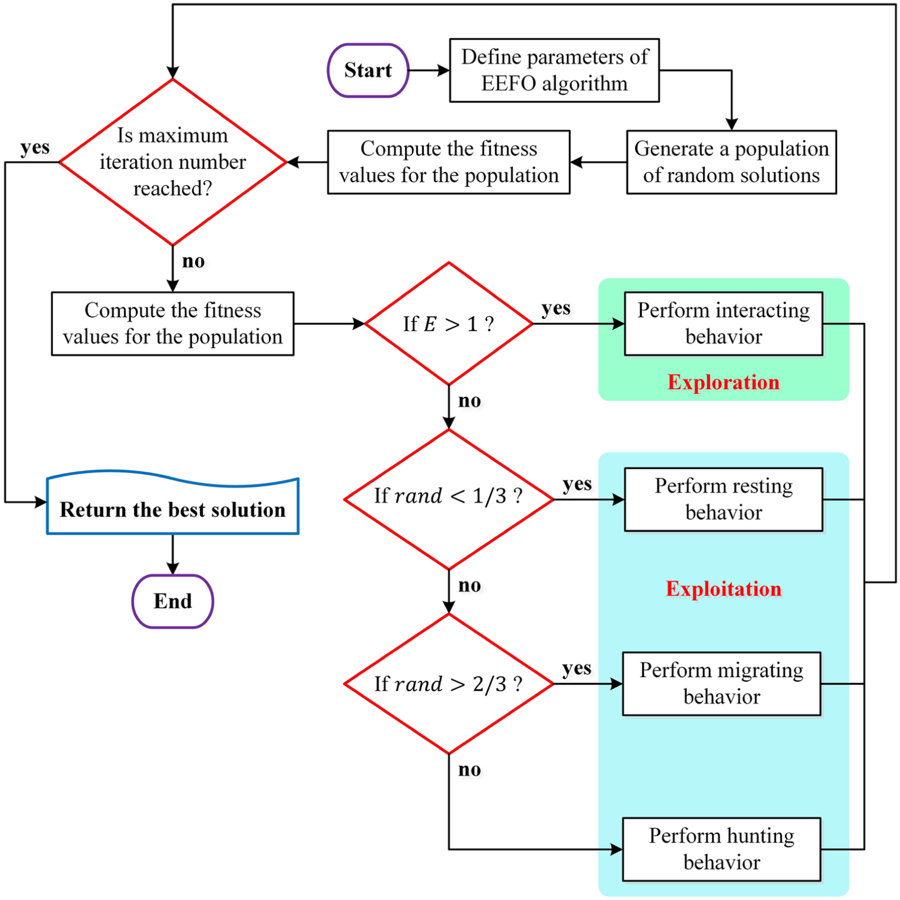
Working mechanism of EEFO.

Recommended EEFO-based cascaded PI-PD controller for buck converter system

This section introduces the cascaded PI-PD control scheme and its effective parameter calibration through using the EEFO algorithm. The primary motivation behind using this control framework is to exploit the complementary benefits of proportional–integral and proportional–derivative actions in a single control loop. Specifically, the PI component helps eliminate steady-state errors by integrating the deviation from the reference, whereas the PD component enhances the dynamic response and stabilizes rapid changes in the output. Figure 5 shows the general block diagram of this cascaded controller. As depicted in Figure 5, the proposed controller cascades two loops: (1) a PI loop, which includes the proportional gain K_P and the integral gain K_I and (2) a PD loop, which includes a second proportional gain K_PP and a derivative gain K_D.

Figure 5.

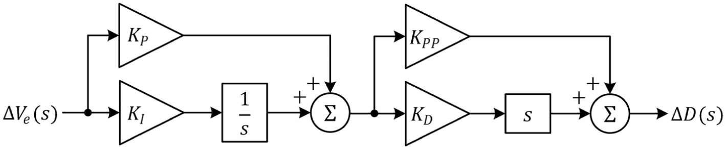
Block diagram of cascaded PI-PD controller.

In Laplace-domain representation, the PI controller is typically defined as $G_{PI} (s) = (K_{P} + (K_{I} / s))$ , while the PD controller takes the form $G_{PD} (s) = (K_{PP} + K_{D} s)$ . When these controllers are arranged in a cascaded structure, the overall controller transfer function (denoted here as $G_{PI - PD} (s)$ ) becomes the product of the two components as given in equation (16).

G_{PI - PD} (s) = (K_{P} + \frac{K_{I}}{s}) \times (K_{PP} + K_{D} s)

(16)

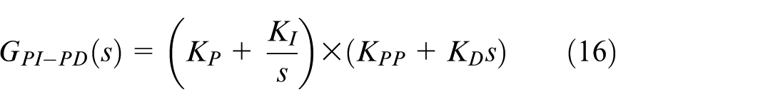
In this expression, $K_{I} / s$ accounts for the integral action that reduces steady-state error, and $K_{D} s$ introduces a predictive behavior that helps counteract rapid output variations. The PI and PD parts are arranged in series so that each component can address distinct aspects of the overall system response. This formulation allows the PI and PD actions to be tuned independently, enhancing control over both the steady-state and dynamic responses. A similar structure has been employed in³⁹ for power system applications, which provides additional theoretical grounding for this approach.

By carefully calibrating K_P, K_I, K_PP, and K_D, one can shape both steady-state and transient performance criteria. Therefore, a crucial step in designing the cascaded PI-PD scheme is choosing the four controller parameters (K_P, K_I, K_PP, and K_D). In this work, the EEFO algorithm automates this search for optimal parameter values. To guide the parameter optimization, an objective function is formulated that balances the trade-off between fast response and minimal overshoot. This multi-criteria function is shown in equation (17):

OF = (1 - ρ) \times m_{os} + ρ \times t_{set}

(17)

where m_os is the maximum percentage overshoot, t_set is the settling time (within a 2% tolerance band), and ρ is a weighting factor between 0 and 1 that prioritizes either overshoot or settling time, depending on the designer’s requirements. In this study, the value of ρ was empirically chosen as 0.95 after conducting extensive evaluations across a range of values (0.1 to 0.99). This setting was found to provide the best trade-off between overshoot suppression and rapid settling, two of the most critical performance requirements for buck converter systems. Lower values of ρ prioritized speed but allowed higher overshoot, while values closer to 1.0 yielded slower responses. The selected value thus ensures a robust and well-damped transient behavior while maintaining fast convergence to the setpoint.

Through iterative evaluations of OF within the EEFO algorithm, the best K_P, K_I, K_PP, and K_D are selected so that the converter output converges to the reference voltage with short settling time and negligible overshoot. makes explicit the multi-objective cost function that the EEFO algorithm attempts to minimize. With proper weighting, designers can focus on reducing overshoot or achieving faster settling, depending on specific requirements.

A schematic of the full control scheme, including both the cascaded PI-PD controller and the EEFO-based tuning mechanism, is illustrated in Figure 6. In this diagram, the Buck converter is driven by pulse-width modulation (PWM), and the output voltage is continuously monitored and fed back to the controller. Inside the controller block, the real-time error between the setpoint and the converter output passes through the PI portion and subsequently the PD portion. The final control signal modulates the duty ratio of the power switch. Meanwhile, the EEFO algorithm runs to fine-tune the four gains (K_P, K_I, K_PP, and K_D).

Figure 6.

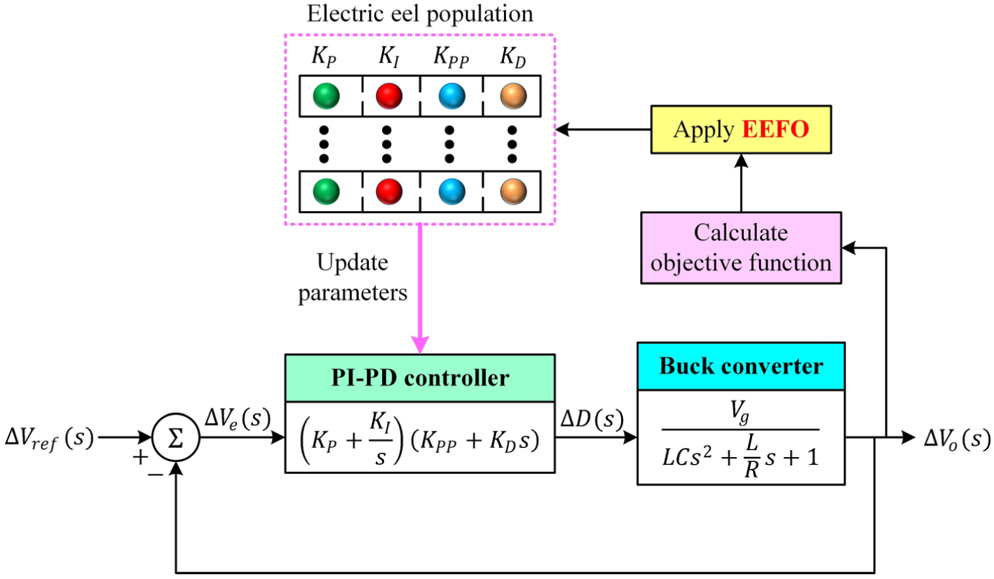
Block diagram of proposed controlled design method for buck converter.

To ensure the highest possible efficiency in the buck converter, the cascaded PI-PD controller gains are constrained within specific intervals. In particular, the proportional gains K_P and K_PP range from 0.01 to 0.5 and 0.01 to 1, respectively, the integral gain K_I spans 0.01–2, and the derivative gain K_D lies between 0.01 and 0.5. These ranges were empirically chosen through extensive preliminary experiments to identify a stable and efficient region in the parameter space, guided by closed-loop stability observations around the nominal operating point and prior tuning experience reported for DC–DC buck converter controllers. The aim was to balance flexibility in exploration with the need to avoid unstable or divergent system responses. Excessively large values of the gains resulted in instability, while overly restrictive bounds limited the optimizer’s performance. Thus, the selected intervals represent a practical compromise that supports robust control behavior and effective parameter tuning using the EEFO algorithm. By defining these operating ranges, the controller is able to maintain both robust transient response and steady-state accuracy, thereby maximizing overall system efficiency. The synergy of cascaded PI and PD loops (coupled with the powerful search ability of the EEFO) provides an effective solution for controlling Buck converters, particularly in applications where quick settling and minimal overshoot are paramount.

Simulation results and discussion

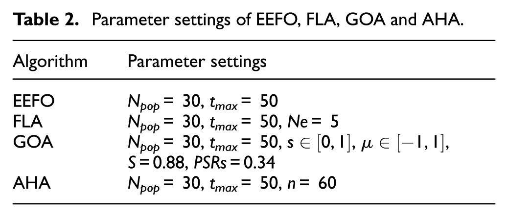
This section presents a broad comparative study aimed at demonstrating the superiority of the proposed EEFO-based PI-PD controller. Several cutting-edge metaheuristic algorithms, including the flood algorithm (FLA),⁴⁰ the gazelle optimization algorithm (GOA),⁴¹ and the artificial hummingbird algorithm (AHA),¹³ were used for benchmarking. Table 2 outlines the specific parameter configurations adopted for these algorithms alongside those for EEFO.³⁶ Here, N_pop signifies the population size, and t_max denotes the maximum number of iterations. To ensure a fair and unbiased comparison, all optimization-based controllers considered in this study were evaluated under identical computational conditions. Specifically, the same population size, maximum number of iterations, objective function formulation, and MATLAB/Simulink simulation environment were used for EEFO and all benchmark metaheuristic algorithms. Furthermore, each comparative controller was independently re-optimized using its corresponding algorithm within its admissible parameter bounds, rather than adopting fixed or reported gains from the literature. This unified evaluation framework ensures that the observed performance differences arise from the intrinsic optimization and control capabilities of each method, rather than from unequal tuning effort or computational advantage.

Table 2.

Parameter settings of EEFO, FLA, GOA and AHA.

Algorithm	Parameter settings
EEFO	N _pop= 30, t_max= 50
FLA	N _pop= 30, t_max= 50, Ne= 5
GOA	N _pop= 30, t_max= 50, $s \in [0, 1]$ , $μ \in [- 1, 1]$ , S=0.88, PSRs=0.34
AHA	N _pop= 30, t_max= 50, n= 60

Comparative assessment using more recent metaheuristic optimization methods

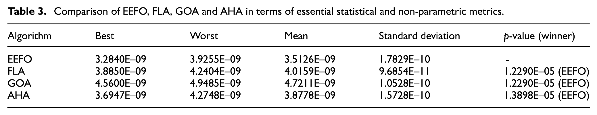
In this subsection, we compare the proposed EEFO-based PI-PD controller against three high-profile optimization algorithms (FLA, GOA, and AHA) to highlight its superior performance in tuning the controller gains. The analyses revolve around both statistical and time-domain performance measures, as well as integral-based error indices. The optimization results obtained by each metaheuristic are compiled in Table 3, which displays the best, worst, and mean objective function values, along with standard deviation. These values give a snapshot of how reliably each algorithm finds high-quality solutions. The EEFO-based controller attains the lowest best cost (3.2840E−09), indicating that among all attempts, EEFO identifies the global optimum (or a near-optimal point) more effectively than the others. Even in its least favorable runs, the EEFO approach remains competitive (3.9255E−09). This outcome underscores the algorithm’s robustness while other methods experience larger fluctuations between runs, EEFO stays closer to its best solution. The mean cost and the spread (standard deviation) of EEFO solutions are also superior, suggesting that the proposed optimizer consistently finds high-quality solutions across repeated trials. A narrow deviation confirms the reliability and repeatability of EEFO’s search process. Hence, Table 3 provides strong evidence that the EEFO method not only yields the most promising individual solutions but also exhibits overall stability and reproducibility compared to FLA, GOA, and AHA.

Table 3.

Comparison of EEFO, FLA, GOA and AHA in terms of essential statistical and non-parametric metrics.

Algorithm	Best	Worst	Mean	Standard deviation	p-value (winner)
EEFO	3.2840E–09	3.9255E–09	3.5126E–09	1.7829E–10	-
FLA	3.8850E–09	4.2404E–09	4.0159E–09	9.6854E–11	1.2290E–05 (EEFO)
GOA	4.5600E–09	4.9485E–09	4.7211E–09	1.0528E–10	1.2290E–05 (EEFO)
AHA	3.6947E–09	4.2748E–09	3.8778E–09	1.5728E–10	1.3898E–05 (EEFO)

To visualize how quickly and effectively each algorithm minimizes the objective function over iterations, Figure 7 plots the convergence curves. The EEFO curve descends more rapidly and levels off at a lower final value than do the curves for FLA, GOA, and AHA. This pattern underscores two critical strengths of EEFO. Firstly, it promptly locates promising regions in the search space, reflecting a well-balanced exploration phase. Secondly, the final plateaus at a smaller objective function value, indicating that once EEFO zeroes in on a viable region, it refines the solution more effectively than competing methods. Therefore, Figure 7 demonstrates the potent combination of swift convergence and robust exploitation capabilities inherent in EEFO.

Figure 7.

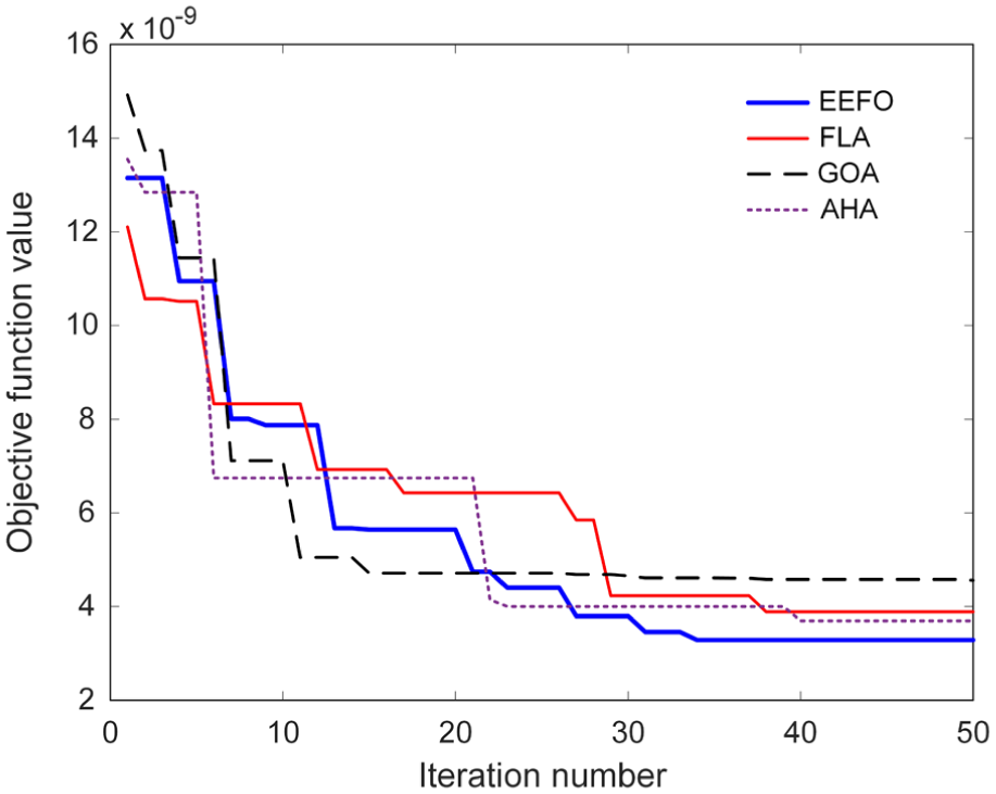
Comparison of the EEFO against other recent algorithms in minimizing the value of OF given in equation (17).

Once each metaheuristic converges, it delivers a set of optimized gains ( $K_{P}, K_{I}, K_{PP} and K_{D}$ ) for the cascaded PI-PD controller. These optimized parameters, displayed in Table 4. The EEFO-derived gains strike a balance that drives the system toward minimal overshoot and rapid settling. Although FLA, GOA, and AHA each propose viable gain values, their solutions tend to yield higher objective function costs, which in turn impact the system’s time-domain performance. In practice, these differences in gain values become especially evident when we examine how the controller responds to reference changes or disturbances, as discussed next.

Table 4.

Optimal values of cascaded PI-PD controller parameters tuned by EEFO, FLA, GOA and AHA.

Algorithm	K _P	K _I	K _PP	K _D
EEFO	0.3852	1.2290	0.8735	0.4297
FLA	0.2918	1.7860	0.9382	0.4795
GOA	0.2718	1.1806	0.7903	0.4386
AHA	0.2953	1.6951	0.6317	0.4982

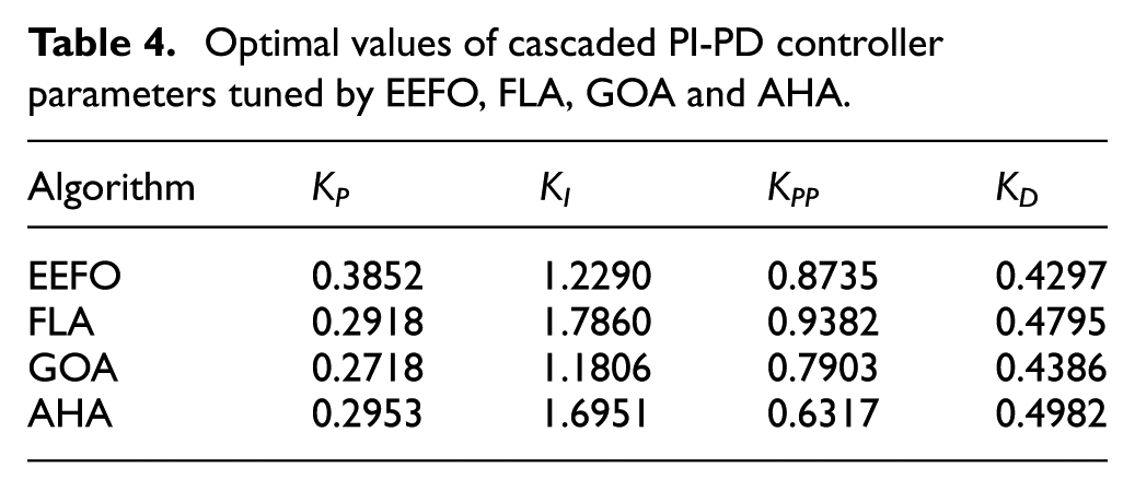
The optimal gain values obtained by EEFO reflect an ideal compromise between rapid transient performance and precise steady-state regulation. The relatively higher value of K_I contributes to fast elimination of steady-state error, while the selected K_D and K_PP support aggressive but well-damped transient correction. The EEFO algorithm identifies this combination by minimizing the objective function defined in equation (17), which emphasizes both overshoot reduction and settling time minimization. This optimized set of gains yields a system response that is not only fast and accurate, but also robust to a wide range of disturbances and uncertainties, as demonstrated in subsequent sections.

An essential criterion for control performance is the behavior of the output voltage under a step change in the reference. Figure 8 illustrates the resulting time-domain waveforms for the four competing algorithms based approaches. The EEFO-tuned PI-PD controller quickly reaches the target voltage, revealing a shorter rise time and faster settling compared to FLA-, GOA-, and AHA-based controllers. Besides, the EEFO-based controller shows negligible steady-state error, which is particularly valuable in applications demanding precise voltage regulation. Therefore, visual inspection confirms that EEFO’s solution manages to hold overshoot at zero, indicating a well-damped response.

Figure 8.

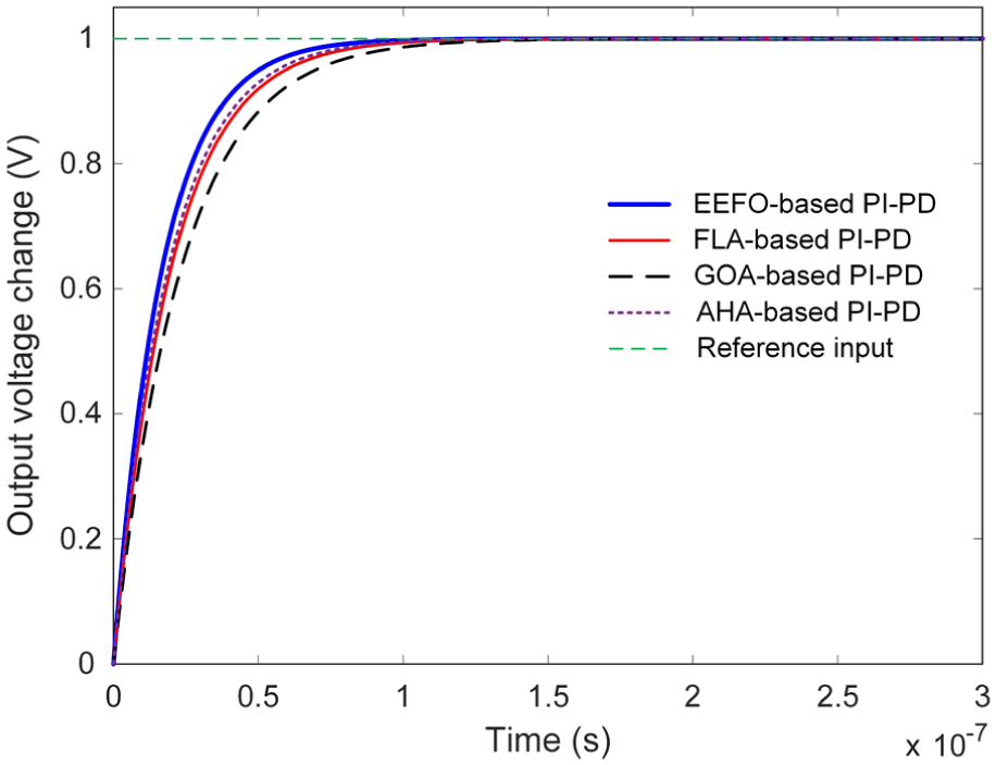
Comparison of the step responses of EEFO, FLA, GOA and AHA approaches.

Table 5 translates these visual impressions into quantitative metrics, listing the settling time (t_set), rise time (t_rise), peak time (t_peak), percentage overshoot (m_os), and steady-state error (e_ss). Notably, EEFO achieves the smallest t_set, t_rise, and t_peak among the four algorithms, accompanied by a practically negligible e_ss. Consequently, its response stands out as both swift and accurate. It is worth noting that the extremely small settling time values reported in Table 5 are obtained under ideal simulation conditions in MATLAB/Simulink, where parasitic effects such as electromagnetic interference (EMI), sensor and ADC delays, dead-time in switching devices, and digital sampling constraints are not present. In real-world buck converter hardware implementations, actual settling times would be longer due to these practical limitations. However, these simulation-based results serve to benchmark the relative performance of the proposed controller under controlled conditions, allowing a fair comparison with other optimization-based tuning strategies. The favorable trends and performance benefits demonstrated by the EEFO-based PI-PD controller (such as faster convergence and zero overshoot) are expected to translate meaningfully to physical prototypes, even if the absolute time constants differ.

Table 5.

Comparison of time response performance metrics of EEFO, FLA, GOA and AHA approaches.

Control method	t _set (s)	t _rise (s)	t _peak (s)	e _ss (%)
EEFO-based PI-PD	6.5680E−08	3.6879E−08	3.3000E−07	0.0030
FLA-based PI-PD	7.7700E–08	4.3629E–08	3.8400E–07	0.0035
GOA-based PI-PD	9.1199E–08	5.1204E–08	4.4300E–07	0.0041
AHA-based PI-PD	7.3893E–08	4.1497E–08	3.6700E–07	0.0033

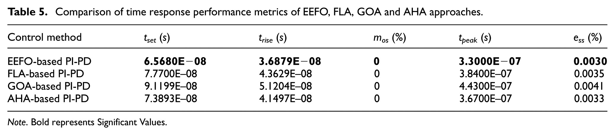
Note. Bold represents Significant Values.

It is worth noting that the exceptionally low values observed for rise time, settling time, and peak time, while highly beneficial in terms of dynamic performance and precision regulation, may introduce certain practical limitations in real-world implementations. For instance, extremely fast control actions can lead to higher switching activity, which may increase power losses and impose thermal and electrical stress on power semiconductor devices. Moreover, such aggressive responses may amplify the effects of sensor noise or exceed the actuation capabilities of physical components. Therefore, while the proposed EEFO-based PI–PD controller demonstrates excellent time-domain behavior in simulations, practical implementations should consider incorporating safety mechanisms such as actuator saturation limits, anti-windup compensation, or filtering strategies to mitigate these potential drawbacks. Addressing these aspects forms a promising direction for future experimental validation.

Although time-response metrics are essential, error-based performance measures provide an additional perspective on control quality. These measures (integral of absolute error (IAE), integral of squared error (ISE), integral of time-absolute error (ITAE), and integral of time-squared error (ITSE)) penalize deviations from the reference over the entire simulation horizon. The respective definitions of these performance metrics are provided in equations (18)–(21).⁴²

F_{IAE} = \int_{0}^{t_{f}} | δ v_{ref} - δ v_{0} | dt

(18)

F_{ISE} = \int_{0}^{t_{f}} {(δ v_{ref} - δ v_{0})}^{2} dt

(19)

F_{ITAE} = \int_{0}^{t_{f}} t | δ v_{ref} - δ v_{0} | dt

(20)

F_{ITSE} = \int_{0}^{t_{f}} t {(δ v_{ref} - δ v_{0})}^{2} dt

(21)

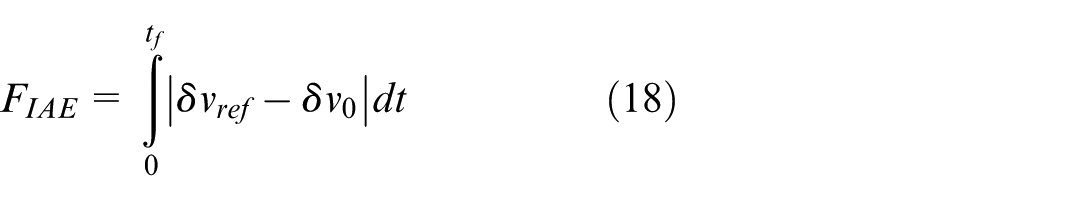
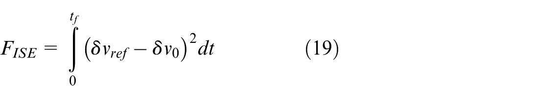
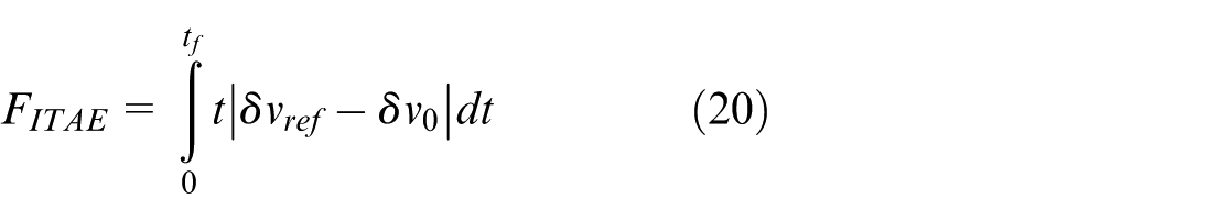
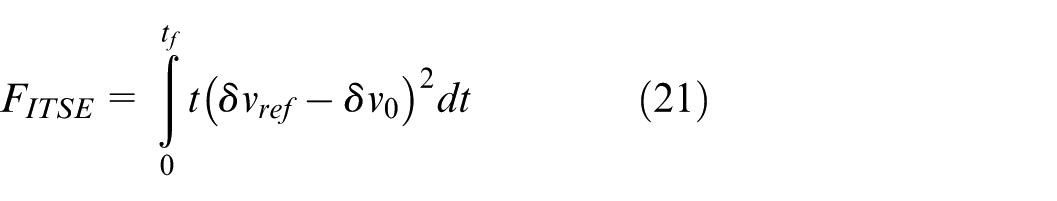
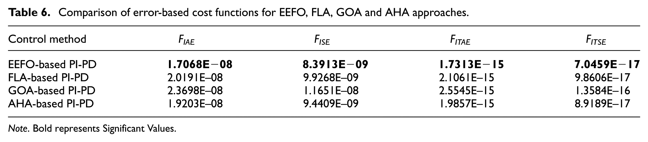
Table 6 compares the performance of each controller according to these criteria. Observations from this table are as follows. The EEFO-based controller registers notably lower values in all four integral indices, implying it corrects errors more swiftly and sustains near-nominal operation for a larger portion of the simulation timeline. The excellent outcomes for integral error measures align well with the improvements previously noted in settling time, overshoot, and steady-state accuracy. This dual confirmation (time-domain metrics and error-based performance metrics) indicates that the EEFO-tuned PI-PD controller provides a more holistic enhancement to system stability and responsiveness relative to other recent metaheuristics.

Table 6.

Comparison of error-based cost functions for EEFO, FLA, GOA and AHA approaches.

Control method	F_IAE	F_ISE	F_ITAE	F_ITSE
EEFO-based PI-PD	1.7068E−08	8.3913E−09	1.7313E−15	7.0459E−17
FLA-based PI-PD	2.0191E–08	9.9268E–09	2.1061E–15	9.8606E–17
GOA-based PI-PD	2.3698E–08	1.1651E–08	2.5545E–15	1.3584E–16
AHA-based PI-PD	1.9203E–08	9.4409E–09	1.9857E–15	8.9189E–17

Note. Bold represents Significant Values.

Comparison with reported PID controlled methods

Having established its advantages over several contemporary metaheuristic-based controllers, we next compared the proposed EEFO-driven PI-PD approach with three exemplary PID controllers found in prior literature, each optimized by a well-regarded algorithm: artificial ecosystem optimization (AEO),²¹ particle swarm optimization (PSO),²¹ and differential evolution (DE).²¹ These methods are widely recognized for their strong performance in DC-DC converter applications and thus offer a demanding benchmark for our cascaded PI-PD scheme. To visualize how quickly and accurately each controller stabilizes the output, Figure 9 depicts the system’s step responses under a reference voltage change. The EEFO-based PI-PD controller transitions to the target voltage in an exceptionally brief interval, clearly surpassing the settling pace of the AEO-, PSO-, and DE-based PID controllers. In practical power electronics, such speed translates to heightened resilience against sudden load swings or abrupt changes in operating conditions. Overshoot can stress converter components and degrade overall system efficiency. While the PID controllers display small but noticeable transient spikes, the EEFO-based PI-PD method exhibits effectively zero overshoot in Figure 9, attesting to its robust damping capabilities and fine-tuned proportional–derivative action. Once settled, the EEFO-based PI-PD holds the output voltage extremely close to the desired level, showing no measurable oscillations or drift. By contrast, the AEO-, PSO-, and DE-based PID designs occasionally display minor lingering fluctuations, albeit within acceptable bounds.

Figure 9.

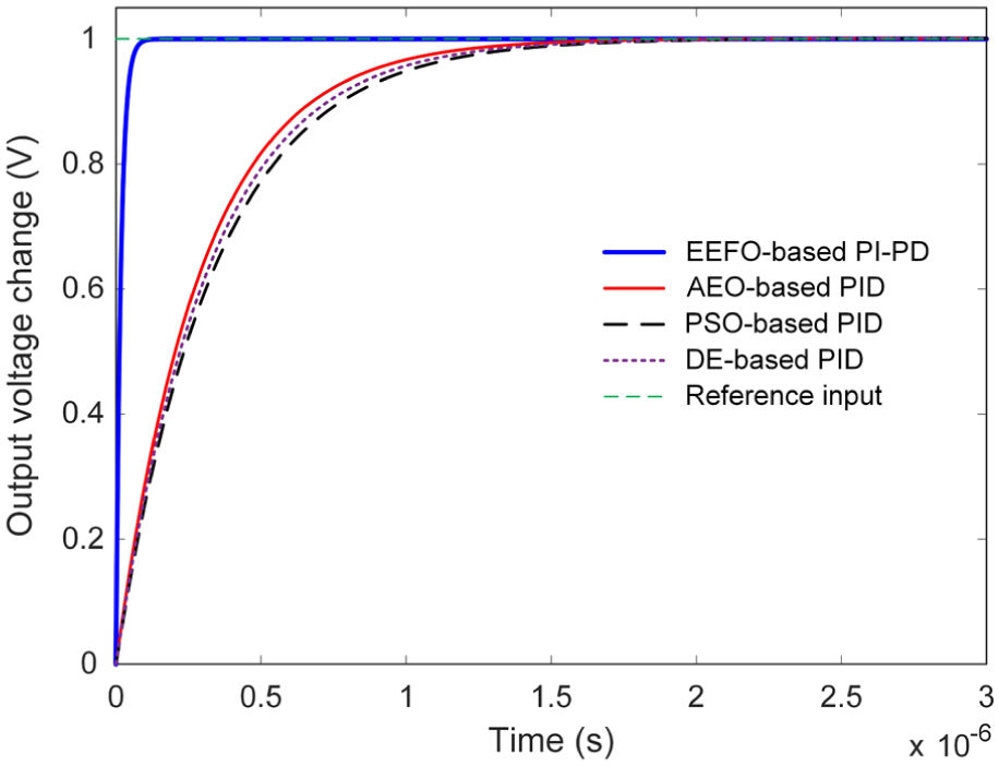
Comparison of the step responses for PID controllers tuned via different approaches.

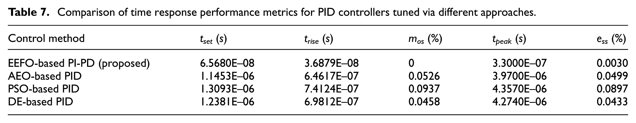
Table 7 translates these observations into quantitative indicators. The EEFO-based PI-PD solution attains a remarkably short settling time of 6.5680E−08. When compared to the microsecond-level times of the other PID controllers, this difference is dramatic, confirming how quickly the proposed method can suppress deviations from the reference. Besides, the EEFO-based controller’s rise time (3.6879E−08) is substantially faster than any of the competing PID algorithms, reflecting an immediate and forceful corrective action. Moreover, the EEFO-based approach outperforms the others by a comfortable margin in terms of peak time, implying well-coordinated proportional and derivative adjustments. The proposed scheme further achieves overshoot of 0%, indicating no excursion beyond the desired setpoint which is a hallmark of stable, well-damped response. Finally, the EEFO-based PI-PD solution maintains an impressively low steady-state deviation (0.0030%), affirming that once the converter output aligns with the setpoint, it remains there with minimal drift.

Table 7.

Comparison of time response performance metrics for PID controllers tuned via different approaches.

Control method	t _set (s)	t _rise (s)	m _os (%)	t _peak (s)	e _ss (%)
EEFO-based PI-PD (proposed)	6.5680E–08	3.6879E–08	0	3.3000E–07	0.0030
AEO-based PID	1.1453E–06	6.4617E–07	0.0526	3.9700E–06	0.0499
PSO-based PID	1.3093E–06	7.4124E–07	0.0937	4.3570E–06	0.0897
DE-based PID	1.2381E–06	6.9812E–07	0.0458	4.2740E–06	0.0433

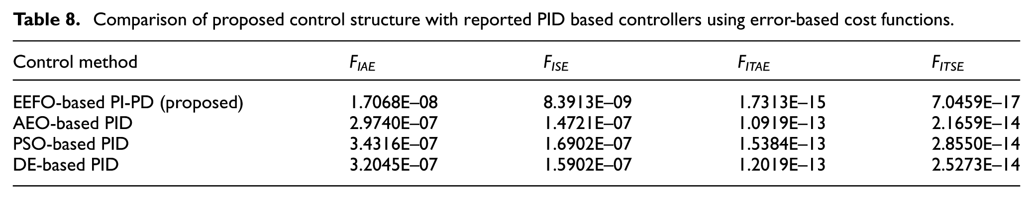
In addition to time-response characteristics, integral error metrics shed light on how controllers perform over the full simulation horizon, penalizing any sustained or substantial deviations from the reference. Table 8 compiles four such measures: IAE, ISE, ITAE, and ITSE. From Table 8, the EEFO-based PI-PD controller yields the smallest values in all four metrics. In practical terms, this result means that the controller quickly suppresses any initial output-voltage mismatch. Because the system remains near the setpoint with no overshoot, the cumulative error remains extremely low over time. Even slight fluctuations that occur late in the response are corrected swiftly, limiting any time-weighted penalty. The pronounced advantage over the AEO-, PSO-, and DE-based PID systems underscores how consistently and comprehensively the EEFO-based PI-PD approach outperforms alternatives, including those previously considered best in class.

Table 8.

Comparison of proposed control structure with reported PID based controllers using error-based cost functions.

Control method	F _IAE	F _ISE	F _ITAE	F _ITSE
EEFO-based PI-PD (proposed)	1.7068E–08	8.3913E–09	1.7313E–15	7.0459E–17
AEO-based PID	2.9740E–07	1.4721E–07	1.0919E–13	2.1659E–14
PSO-based PID	3.4316E–07	1.6902E–07	1.5384E–13	2.8550E–14
DE-based PID	3.2045E–07	1.5902E–07	1.2019E–13	2.5273E–14

Comparison with reported PIDA controlled methods

In addition to the commonly studied PID controllers, certain applications adopt PID acceleration (PIDA) control architectures to achieve more refined transient and steady-state performance in power electronic converters. This subsection demonstrates how the proposed EEFO-driven PI-PD regulator fares against leading PIDA-based solutions (specifically those tuned via manta ray foraging optimization (MRFO),⁴³ arithmetic optimization algorithm (AOA),⁴³ and Lévy flight distribution (LFD).⁴³ These algorithms have each shown promising results in prior literature for managing DC-DC buck converters.

Figure 10 compares the voltage step responses of the MRFO-based PIDA, AOA-based PIDA, LFD-based PIDA, and the proposed EEFO-based PI-PD controllers. The EEFO-based PI-PD approach achieves the reference voltage almost instantaneously, visibly outpacing the three PIDA controllers’ convergence times. While MRFO-, AOA-, and LFD-based PIDA designs do eventually track the setpoint, they exhibit relatively longer rise and settling intervals. Although some of the PIDA controllers maintain overshoot near zero, their transient trajectories display more noticeable undershoot (or “sag”) and a slower ramp to the final voltage. In contrast, the proposed method transitions fluidly to the setpoint, indicating a well-calibrated balance between speed and damping. The final steady-state levels for MRFO-, AOA-, and LFD-based PIDA controllers each exhibit minor residual deviations or longer tails before stabilizing. By comparison, the EEFO-based PI-PD rapidly locks onto the reference with minimal oscillatory behavior.

Figure 10.

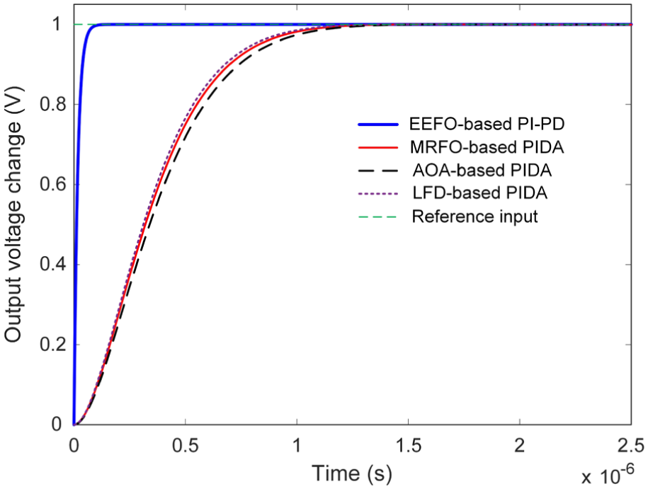
Comparison of the step responses for PIDA controllers tuned via different approaches.

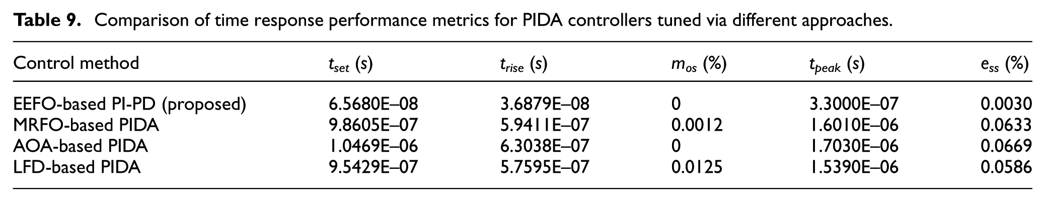
To objectively validate these observations, Table 9 presents standard transient-performance indicators: settling time, rise time, overshoot, peak time, and steady-state error. The EEFO-based PI-PD controller reports an extremely brief settling time (6.5680E−08) and an equally impressive rise time (3.6879E−08), both of which are markedly shorter than those observed for the PIDA controllers. In many applications, even small overshoots can adversely affect component life or downstream circuitry. Not only does the proposed approach exhibit zero overshoot, but it also outperforms two of the three PIDA controllers that show small but non-negligible overshoot levels. Once the system has settled, the EEFO-based PI-PD stands out with a steady-state deviation of approximately 0.0030%. By contrast, the PIDA controllers report higher error magnitudes, indicating that they require more time to converge precisely to the reference or continue to exhibit minor fluctuations even after stabilization.

Table 9.

Comparison of time response performance metrics for PIDA controllers tuned via different approaches.

Control method	t _set (s)	t _rise (s)	m _os (%)	t _peak (s)	e _ss (%)
EEFO-based PI-PD (proposed)	6.5680E–08	3.6879E–08	0	3.3000E–07	0.0030
MRFO-based PIDA	9.8605E–07	5.9411E–07	0.0012	1.6010E–06	0.0633
AOA-based PIDA	1.0469E–06	6.3038E–07	0	1.7030E–06	0.0669
LFD-based PIDA	9.5429E–07	5.7595E–07	0.0125	1.5390E–06	0.0586

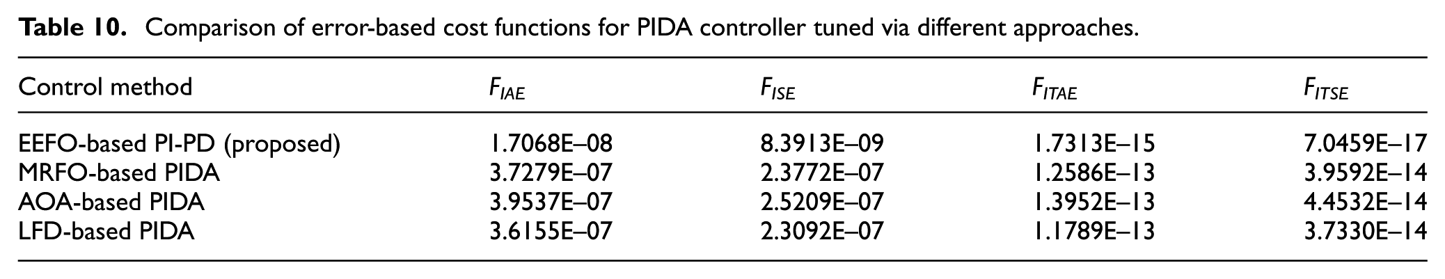
While time-domain characteristics emphasize overshoot and settling behavior, error-based performance metrics provide a fuller picture of how the controller handles deviations across the entire simulation timeframe. Consequently, Table 10 compares four integrated error measures (IAE, ISE, ITAE, and ITSE) among the four controllers. The EEFO-based PI-PD maintains notably smaller values for all integral cost functions. This indicates it not only settles more rapidly but also sustains precise voltage control during steady-state operation, minimizing error accumulation in both early and later stages of the response. Because ITAE and ITSE incorporate time weighting, they penalize any persistent misalignment between the output and reference. The proposed controller’s minimal integral penalties attest to its ability to swiftly correct initial transients and then remain close to the set point, avoiding large or protracted deviations.

Table 10.

Comparison of error-based cost functions for PIDA controller tuned via different approaches.

Control method	F _IAE	F _ISE	F _ITAE	F _ITSE
EEFO-based PI-PD (proposed)	1.7068E–08	8.3913E–09	1.7313E–15	7.0459E–17
MRFO-based PIDA	3.7279E–07	2.3772E–07	1.2586E–13	3.9592E–14
AOA-based PIDA	3.9537E–07	2.5209E–07	1.3952E–13	4.4532E–14
LFD-based PIDA	3.6155E–07	2.3092E–07	1.1789E–13	3.7330E–14

Comparison with reported FOPID controlled methods

In some applications, fractional-order PID (FOPID) controllers are employed to provide additional tuning flexibility over conventional PID schemes. This subsection illustrates how the proposed EEFO-based PI-PD controller compares against three high-performing FOPID controllers optimized by different algorithms: Harris hawks optimization (HHO),⁴⁴ cooperation search algorithm (CSA),³³ and a hybrid Lévy flight distribution–simulated annealing (LFDSA).⁴⁵ These methods have each demonstrated impressive results in earlier DC-DC converter studies.

To highlight how quickly and accurately each controller stabilizes the output voltage, Figure 11 presents the system’s time-domain waveforms for a step change in reference. The EEFO-based PI-PD regulator swiftly converges on the target voltage, visibly faster than the HHO-, CSA-, and LFDSA-based FOPID controllers. This rapid tracking is particularly beneficial where sudden load or input perturbations demand a prompt corrective response. As in previous comparisons, the EEFO-based PI-PD scheme attains essentially zero overshoot. By contrast, while the FOPID designs in Figure 11 generally keep overshoot modest, they still require longer transitions before settling into steady operation. Once it locks onto the reference, the proposed controller remains tightly aligned, showing negligible oscillations or drift. Meanwhile, the FOPID alternatives tend to display minor extended transients or a slightly slower approach to final voltage levels.

Figure 11.

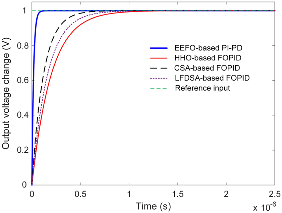
Comparison of the step responses for FOPID controllers tuned via different approaches.

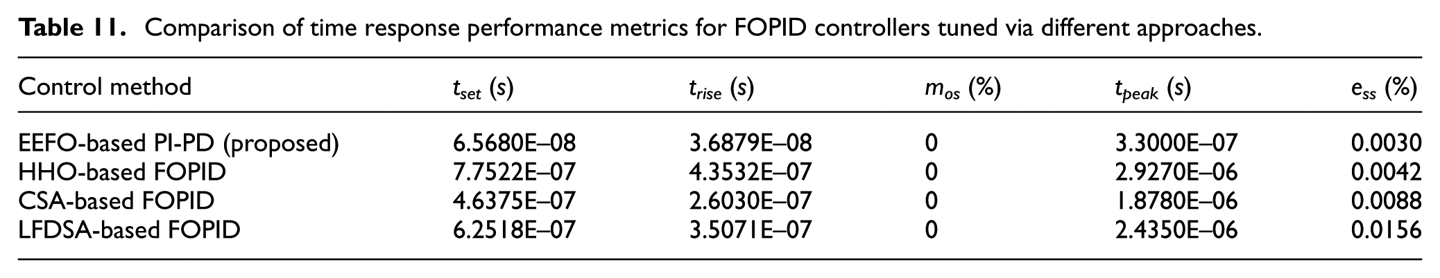
To quantify the trends from Figure 11, Table 11 enumerates key transient response parameters: settling time, rise time, overshoot, peak time, and steady-state error. Noteworthy observations include: The EEFO-based solution’s settling time (6.5680E−08) and rise time (3.6879E−08) are significantly shorter than those of the HHO-, CSA-, and LFDSA-based FOPID controllers. This rapidity translates to minimized transient disturbances and a near-instantaneous approach to nominal voltage. Overshoot not only risks exceeding component tolerances but can also lead to extra voltage stress. The proposed controller avoids these dangers entirely by holding 0% overshoot once the output settles, the EEFO-based PI-PD consistently maintains a minuscule steady-state error (0.0030%). This suggests that after the initial transient, the converter remains highly stable and closely follows the desired voltage.

Table 11.

Comparison of time response performance metrics for FOPID controllers tuned via different approaches.

Control method	t _set (s)	t _rise (s)	t _peak (s)	e _ss (%)
EEFO-based PI-PD (proposed)	6.5680E–08	3.6879E–08	3.3000E–07	0.0030
HHO-based FOPID	7.7522E–07	4.3532E–07	2.9270E–06	0.0042
CSA-based FOPID	4.6375E–07	2.6030E–07	1.8780E–06	0.0088
LFDSA-based FOPID	6.2518E–07	3.5071E–07	2.4350E–06	0.0156

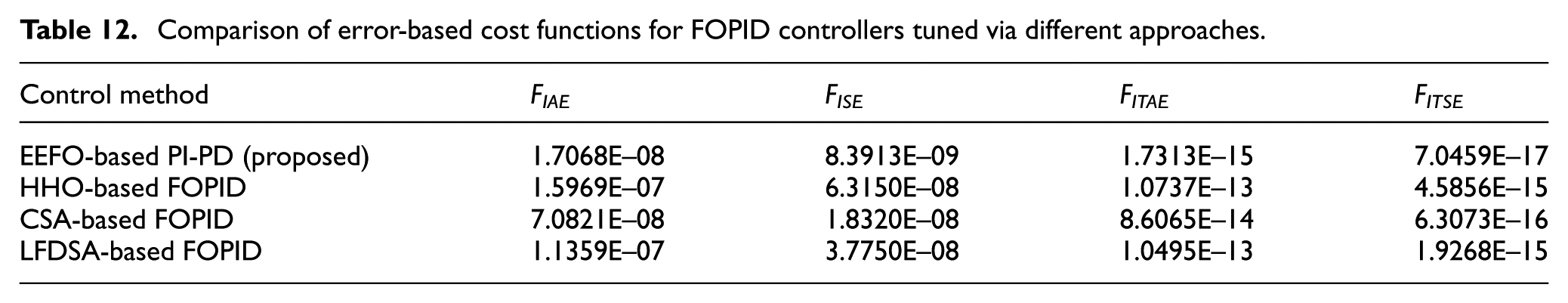
Although time-response indicators supply a clear snapshot of transient performance, error-based measures capture the accumulated error over the entire operational span. Table 12 compares the IAE, ISE, ITAE, and ITSE for each FOPID controller and the proposed PI-PD strategy. Across all four measures, the EEFO-based controller registers the smallest numerical results. This points to its ability to not only settle swiftly but also maintain tight control thereafter, preventing large or enduring deviations. By quickly eradicating any transient error and maintaining a stable setpoint lock, the proposed controller keeps the integrated error close to zero. This behavior is particularly evident in the time-weighted metrics (ITAE, ITSE), which penalize prolonged misalignment from the setpoint. These advantages indicate that, under both transient and sustained operating conditions, the EEFO-based PI-PD scheme outperforms HHO-, CSA-, and LFDSA-tuned FOPID controllers, offering a more comprehensive improvement in converter regulation.

Table 12.

Comparison of error-based cost functions for FOPID controllers tuned via different approaches.

Control method	F _IAE	F _ISE	F _ITAE	F _ITSE
EEFO-based PI-PD (proposed)	1.7068E–08	8.3913E–09	1.7313E–15	7.0459E–17
HHO-based FOPID	1.5969E–07	6.3150E–08	1.0737E–13	4.5856E–15
CSA-based FOPID	7.0821E–08	1.8320E–08	8.6065E–14	6.3073E–16
LFDSA-based FOPID	1.1359E–07	3.7750E–08	1.0495E–13	1.9268E–15

Robustness of EEFO-based cascaded PI-PD controller under non-ideal conditions

While the preceding sections focus primarily on idealized simulations, real-world DC-DC converter systems often operate under less predictable circumstances. External disturbances, measurement noise, sudden reference shifts, time delays, and parameter uncertainties in circuit elements can all undermine stability and performance.²⁵ To address these challenges, we systematically examine the robustness of the proposed EEFO-based PI-PD controller in the presence of such non-ideal conditions. A schematic depiction of the controller operating in a non-ideal environment is illustrated in Figure 12. In this extended model, the Buck converter is influenced by various real-world factors (abrupt changes in setpoints, injection of random or systematic noise, temporal lags in the feedback loop, and deviations in component values (e.g. inductance, capacitance)). By capturing these elements within the simulation framework, we can determine how effectively the EEFO-based controller adapts and maintains regulation when conditions deviate from the nominal design assumptions.

Figure 12.

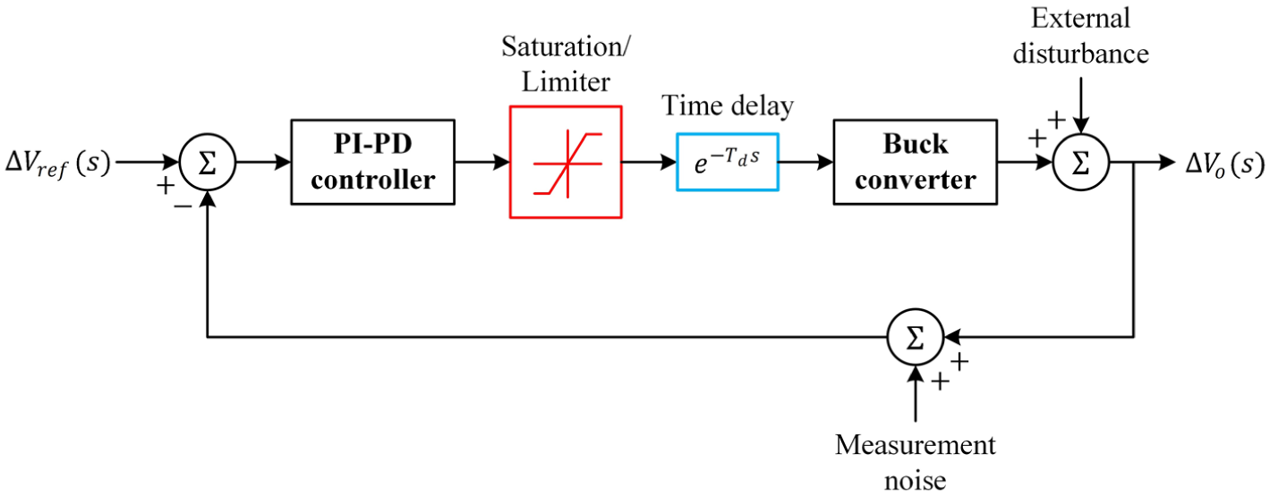
Block diagram of the proposed controlled design method subjected to non-ideal conditions.

As illustrated, the proposed controller continuously monitors the converter output and attempts to hold it near the desired setpoint, despite potential sources of disturbance or error feeding into the system. The following subsections describe the various analyses used to validate the controller’s resilience for effect of variable setpoints, nonlinearities, time delay and parametric uncertainty. Through these targeted investigations, we demonstrate that the EEFO-optimized PI-PD controller not only excels in idealized simulations but also remains robust across an array of practical scenarios. Each subsequent subsection details a specific source of non-ideality, describes the experimental setup, and interprets the corresponding results, reinforcing the claim that the proposed control methodology delivers strong resilience and high efficiency under realistic operating conditions.

It should be noted that the robustness analysis presented in this section is intended to provide a structured and representative validation of the proposed controller under commonly encountered non-ideal operating conditions in DC–DC buck converter systems. While more complex coupled disturbances (such as simultaneous input voltage sags combined with abrupt load variations) may arise in practical deployments, the scenarios investigated herein already encompass multiple interacting non-idealities, including disturbance injection with measurement noise, time-delay effects, and parametric uncertainty. These tests collectively impose substantial stress on the control loop and are sufficient to evaluate fundamental robustness characteristics. Furthermore, robustness assessments were conducted exclusively for the proposed EEFO-based cascaded PI–PD controller to highlight its absolute disturbance-rejection capability. Since all benchmark controllers were already optimized and comparatively evaluated under identical conditions in Section 5, additional robustness comparisons were omitted to avoid redundancy and excessive complexity. Nevertheless, extending the robustness framework to include coupled disturbance scenarios and comparative robustness analyses constitutes a meaningful direction for future research.

Effect of variable setpoints

In many real-world scenarios, a DC-DC buck converter must adapt to changing output voltage requirements rather than maintaining a single fixed setpoint. To assess how effectively the proposed EEFO-based PI-PD controller handles such dynamic demands, this subsection introduces abrupt shifts in the reference voltage and observes the controller’s transient and steady-state behavior. Figure 13 demonstrates the response of the converter output as the reference changes stepwise. Even under significant deviations from the nominal setpoint, the controller swiftly re-establishes the output voltage to the newly specified level. The controller reacts with negligible delay, reflecting how efficiently the PI and PD loops compensate for sudden increases or decreases in the target voltage. This speed of response ensures minimal downtime and maintains power quality. Despite abrupt transitions, overshoot remains low or absent, indicating that the coordinated action of the PI loop and PD loop effectively damps any oscillatory tendencies. Once the controller settles at the new setpoint, the steady-state error is effectively negligible. As depicted in Figure 13, the EEFO-based PI-PD controller demonstrates robust adaptability, maintaining output stability through each step change without excessive overshoot or protracted settling. This characteristic is especially valuable in applications where the load demand or operating conditions shift frequently, such as in distributed power systems and renewable energy setups.

Figure 13.

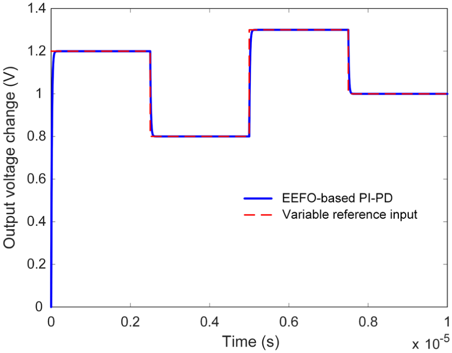
Response of the proposed controller to a changing input reference.

Effect of nonlinearities

Realistic buck converter environments rarely operate in perfectly linear domains. Instead, they often encounter external disturbances such as load fluctuations or grid-side transients and inherent measurement noise from sensors or instrumentation. Both phenomena can introduce additional oscillations or inaccuracies, complicating the controller’s ability to maintain precise regulation. To evaluate the robustness of our EEFO-based PI-PD controller under these conditions, we inject disturbance and noise profiles into the system and observe the resulting output trajectories. Figure 14 depicts two principal sources of nonlinearity. Figure 14(a) represents a sudden deviation in the load or input supply, mimicking real-world disruptions such as abrupt load steps or brief grid anomalies. On the other hand, Figure 14(b) emulates random sensor noise superimposed on the voltage feedback signal, reflecting imperfect sensing or electrical interference common in high-frequency converter circuits.

Figure 14.

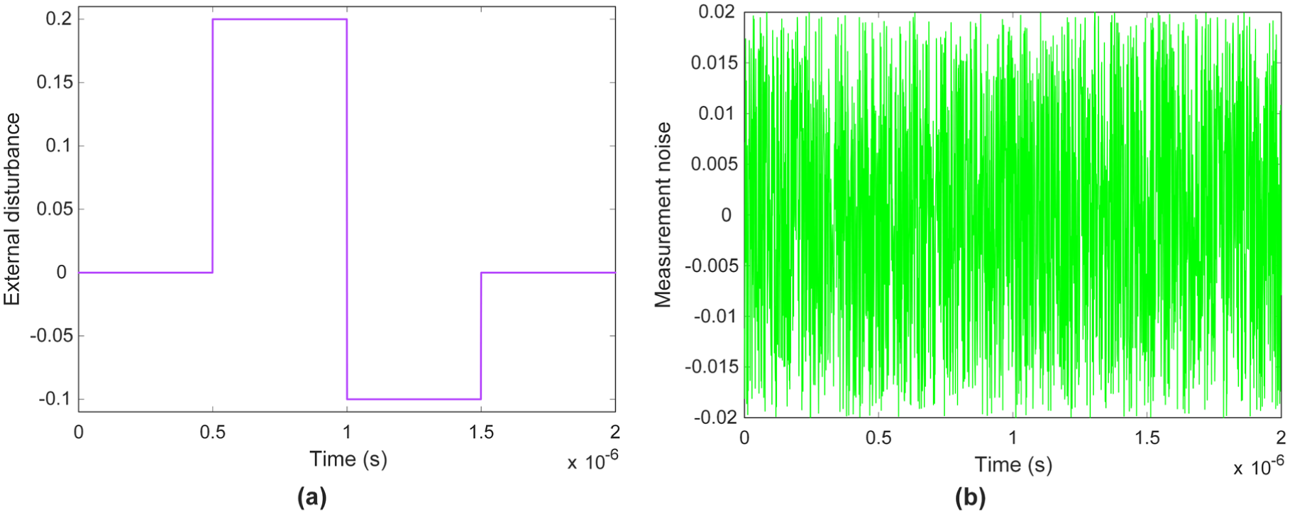
External disturbance (a) and measurement noise (b).

Figure 15 illustrates the actual output voltage profile when the controller faces these combined non-idealities (disturbance plus noise). Despite an initial surge caused by the introduced disturbance, the proposed controller swiftly damps out high-frequency ripples and prevents them from propagating into protracted overshoot. This quick recovery reflects the cascade structure’s ability to handle large error signals effectively, with the PI loop tracking offsets and the PD loop curbing abrupt rate changes. Once the immediate transient subsides, the system remains closely aligned to the desired voltage. The minor fluctuations observed early on are short-lived, indicating strong loop compensation and minimal drift or hunting around the reference. Even though measurement noise complicates accurate feedback signals, the controller continues to track the setpoint without significant jitter or sustained error. This robustness is crucial in industrial and power electronics domains where noise contamination can be unavoidable. These results confirm that the EEFO-based PI-PD controller not only excels under ideal test scenarios but also maintains strong performance amidst realistic nonlinear challenges. By rapidly attenuating disturbances and ignoring minor sensor irregularities, the controller ensures stable, precise output regulation. In the subsequent subsections, we explore additional tests (including time delays and parametric uncertainties) to further validate this robust performance across a broader spectrum of real-world operating conditions.

Figure 15.

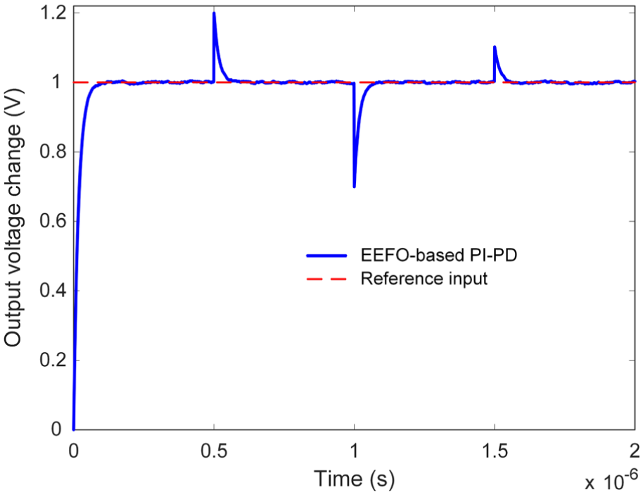
Variation of output voltage with time subject to nonlinear effects.

Effect of time delay

In practical power electronics systems, communication and processing latencies (arising from digital controllers, signal filtering, or data transmission) can introduce time delays that degrade control performance. Even seemingly minor lags in reading sensor data or updating pulse-width modulation (PWM) signals can limit how promptly the system responds to perturbations or reference changes, thereby influencing overall stability and efficiency. To examine the robustness of the proposed EEFO-based PI-PD controller under these conditions, we introduce incremental delays into the feedback loop and observe how effectively the controller continues to regulate the output voltage. Figure 16 shows the converter’s response for three scenarios. First is no delay which represents the ideal baseline, with instantaneous feedback of the output voltage. Second is moderate delay which emulates minor lags typical of digital controllers and sensor filtering. The last one is substantial delay which reflects more significant system latencies or communications overhead which are conditions that can arise in geographically distributed or complex power networks.

Figure 16.

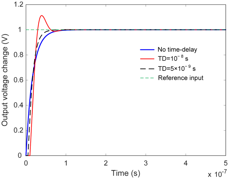
Temporal delayed reference signal tracking of output voltage.

Even under substantial time lags, the EEFO-based PI-PD controller maintains voltage tracking without destabilizing oscillations. While longer delays do extend the settling duration slightly, the system remains well-damped and avoids significant overshoot or undershoot. Compared with many conventional controllers, which can exhibit heightened overshoot or even risk instability when faced with latencies, the proposed scheme continues to converge to the setpoint with nominal overshoot. The well-coordinated interplay of PI and PD actions appears to counteract the phase shifts introduced by the delay. As the time lag increases, the controller adjusts its dynamic response without abrupt transitions or large deviations. This adaptability indicates that the EEFO-driven parameter tuning confers a degree of tolerance for moderate latency which is a frequent concern in digital control systems. In summary, the EEFO-optimized PI-PD controller exhibits robust behavior under varying degrees of time delay, preserving stable and efficient voltage regulation. This resilience is vital in real-world applications where controller computations, sensor filtering, or communications overhead can introduce nontrivial latencies. Subsequent analyses build on these findings, probing further potential deviations such as component tolerance changes to establish a more comprehensive view of the controller’s performance envelope. Further simulations revealed that the proposed controller maintains stable performance up to a maximum feedback loop delay of approximately $TD = 2.5 \times 10^{- 8} s$ . Beyond this threshold, system stability begins to deteriorate, with noticeable increases in overshoot and settling time. However, this delay value is considered conservatively high for buck converter systems and typically exceeds the delay durations encountered in practical applications. This result reinforces the robustness of the EEFO-based PI-PD controller against realistic communication and computation latencies.

Effect of parametric uncertainty

Real-world buck converters are rarely assembled with perfectly calibrated passive components, and slight deviations in parameters such as inductance and capacitance can introduce additional challenges to output regulation. To examine the resilience of the proposed controller under such conditions, we intentionally varied the nominal inductance and capacitance values and investigated how these shifts influence system stability and efficiency. Table 13 summarizes four representative scenarios: (i) increasing the capacitor value by 10%, (ii) decreasing the capacitor value by 10%, (iii) increasing the inductor value by 15%, and (iv) decreasing the inductor value by 15%.

Table 13.

Variation of parameters of system circuit elements.

Scenario	Parameter	Change amount
A	L	$- 15 %$
B	L	$+ 15 %$
C	C	$- 10 %$
D	C	$+ 10 %$

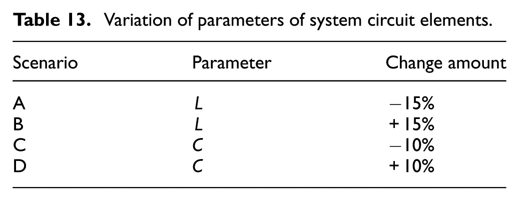
Figure 17 provides the corresponding output voltage profiles in each scenario, while Table 14 lists key performance metrics, namely the rise time, settling time, overshoot, peak time, and steady-state error. Despite these deliberate parameter offsets, the controller consistently maintained regulation very close to the nominal behavior. As shown in Figure 17, variations in inductance or capacitance cause only minor shifts in the transient and steady-state responses. Crucially, none of the scenarios exhibit instability or large overshoot, underscoring the robustness of the proposed design.

Figure 17.

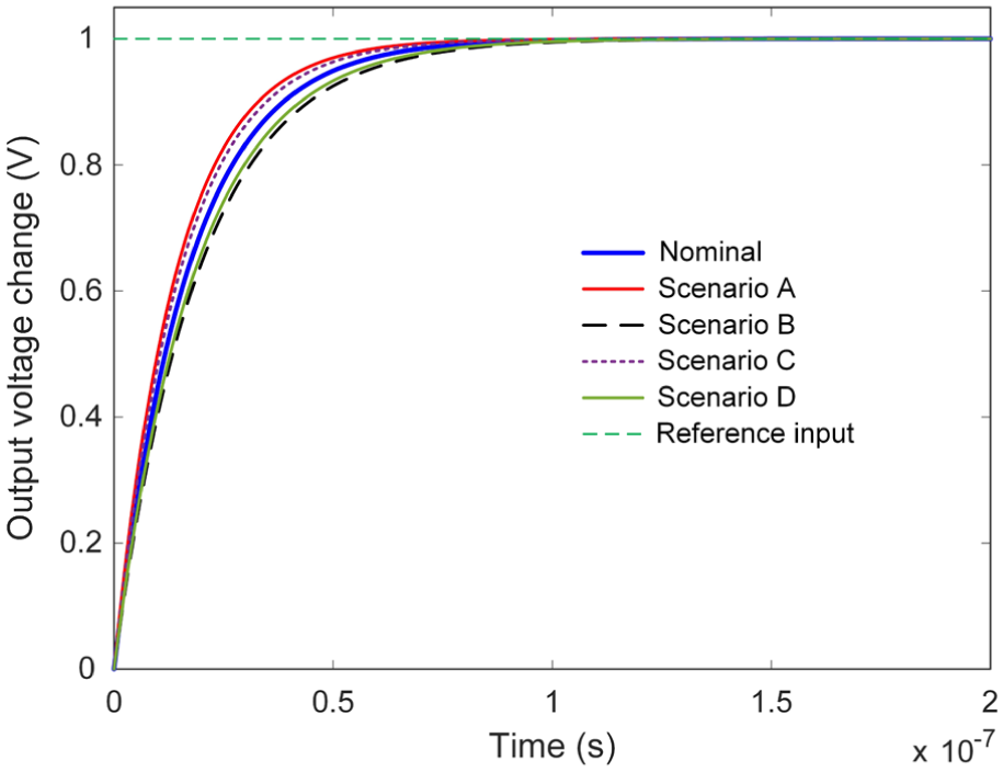
Following the reference signal of the output voltage in case of changes in parameter values.

Table 14.

Comparison of time response performance metrics.

Scenario	t _set (s)	t _rise (s)	t _peak (s)	e _ss (%)
Nominal	6.5680E–08	3.6879E–08	3.3000E–07	0.0030
A	5.5825E–08	3.1341E–08	2.8300E–07	0.0025
B	7.5534E–08	4.2415E–08	3.7700E–07	0.0034
C	5.9109E–08	3.3187E–08	2.9900E–07	0.0030
D	7.2245E–08	4.0570E–08	3.6200E–07	0.0030

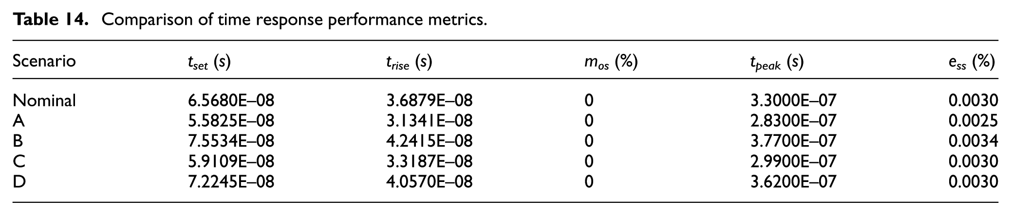
The time-domain performance data in Table 14 corroborate these observations: although each modification in the component values produces slight differences in rise and settling times, the controller’s steady-state accuracy remains virtually unaffected. These results collectively indicate that the EEFO-based cascaded PI-PD controller is not only adept at handling external perturbations and measurement noise but also maintains excellent robustness against moderate parameter drifts. By reliably stabilizing the output even when component values stray from their nominal ratings, the controller demonstrates considerable practical appeal for applications in which component tolerances or aging effects are unavoidable.

In addition to the four test cases shown in Table 13, it is important to note that the proposed EEFO-based PI-PD controller is highly scalable due to its optimization-driven nature. While this study primarily investigates a widely adopted standard buck converter configuration, the same control design procedure can be seamlessly applied to systems operating at higher power levels, different switching frequencies, or modified passive component values. The robustness analysis under varied inductance and capacitance parameters already demonstrates the controller’s resilience to such deviations. Moreover, since the EEFO algorithm operates over a bounded parameter space, it can be retrained for new configurations by redefining the dynamic model and adjusting the objective function as needed. This adaptability ensures that the proposed controller remains viable for a wide range of practical converter designs.

Conclusion

This work introduces a novel control strategy by deploying, for the first time, a cascaded PI–PD controller optimized via the EEFO in the context of DC–DC buck converters. The originality lies in both the structural novelty of the cascaded control design and the unique application of a nature-inspired metaheuristic that has not been previously explored in this domain. The two-loop structure effectively capitalizes on the combined strengths of PI and PD actions: the PI component targets low steady-state errors while the PD component mitigates abrupt transients. For proper parameter calibration and ensuring system performance, EEFO is employed as an effective optimizer. Through extensive simulations and comparisons with multiple cutting-edge optimizers and established controller types, the proposed EEFO-based PI–PD approach consistently demonstrated faster transient settling and lower error accumulations than existing methods. A key observation is how swiftly the converter stabilizes at the desired voltage level, with zero overshoot and minimal steady-state deviation. These favorable dynamics arise from the precise balance of proportional and derivative terms, fine-tuned by EEFO’s robust search mechanism. The controller also maintained remarkable resilience against realistic non-ideal conditions, including abrupt changes in reference voltage, external load disturbances, sensor noise, time delays, and moderate parameter variations in inductance and capacitance. In all these scenarios, the output voltage remained tightly regulated, underscoring the controller’s versatility and reliability.

Beyond validating its capability to provide high-performance regulation under varied conditions, this study highlights the scalability and adaptability of our proposed approach. Its straightforward integration into other power electronic configurations opens avenues for broader industrial deployment, particularly where rapid response and stable operation are paramount. While the current study is centered on a single-converter configuration to rigorously demonstrate the core performance and robustness of the proposed EEFO-based PI–PD controller, the underlying methodology is not limited to this setting. Owing to its modular structure and optimization-driven tuning process, the approach is inherently scalable and well-suited for extension to multi-converter architectures and grid-connected environments.

Footnotes

Acknowledgements

The authors would like to express their sincere gratitude to Lukas Prokop and Stanislav Misak for their exceptional supervision, project administration, and overall guidance throughout the course of this project. Their expertise and support were instrumental to its success.

ORCID iDs

Davut Izci

Ievgen Zaitsev

Author contributions

Davut Izci, Edip Ertuğrul, Serdar Ekinci: Conceptualization, Methodology, Software, Visualization, Investigation, Writing - Original draft preparation, Mohit Bajaj, Mostafa Jabari: Data curation, Validation, Supervision, Resources, Writing - Review & Editing. Emre Çelik, Ievgen Zaitsev, Vojtech Blazek: Project administration, Funding, Supervision, Resources, Writing - Review & Editing.

Funding

The authors disclosed receipt of the following financial support for the research, authorship, and/or publication of this article: This research is funded by European Union under the REFRESH—Research Excellence For Region Sustainability and High-Tech Industries Project via the Operational Program Just Transition under Grant CZ.10.03.01/00/22_003/0000048; in part by the National Center for Energy II and ExPEDite Project a Research and Innovation Action to Support the Implementation of the Climate Neutral and Smart Cities Mission Project TN02000025; and in part by ExPEDite through European Union’s Horizon Mission Program under Grant 101139527.

Declaration of conflicting interests

The authors declared no potential conflicts of interest with respect to the research, authorship, and/or publication of this article.

Data availability statement

All relevant data are within the manuscript. The collection and analysis method complied with the terms and conditions for the source of the data.

References

Maksimovic

Stankovic

Thottuvelil

, et al. Modeling and simulation of power electronic converters. Proc IEEE 2001; 89: 898–912.

Izci

Ekinci

A novel improved version of hunger games search algorithm for function optimization and efficient controller design of buck converter system. e-Prime 2022; 2: 100039.

Aryan

Raja

Mehta

, et al. A resilient tri-parametric fractional frequency control for cybersecurity threats amid latency. IEEE Trans Ind Appl 2025; 61: 5597–5611.

Aryan

Raja

GL.

Design and analysis of novel QOEO optimized parallel fuzzy FOPI-PIDN controller for restructured AGC with HVDC and PEV. Iran J Sci Technol Trans Electr Eng 2022; 46: 565–587.

Kumari

Aryan

Raja

, et al. Dual degree branched type-2 fuzzy controller optimized with a hybrid algorithm for frequency regulation in a triple-area power system integrated with renewable sources. Prot Control Mod Power Syst 2023; 8: 48.

Anand

Aryan

Kumari

, et al. Type-2 fuzzy-based branched controller tuned using arithmetic optimizer for load frequency control. Energy Sour A Recov Utilization Environ Effects 2022; 44: 4575–4596.

Mukherjee

Raja

Kundu

, et al. Modified augmented fractional order control schemes for cart inverted pendulum using constrained Luus-Jaakola optimisation. Int J Model Identif Control 2021; 38: 367.

Izci

Ekinci

Jabari

, et al. A novel gudermannian function-driven controller architecture optimized by starfish optimizer for superior transient performance of automatic voltage regulation. Biomimetics 2025; 11: 7.

Nanyan

Ahmad

Hekimoğlu

Optimal PID controller for the DC-DC buck converter using the improved sine cosine algorithm. Results Control Opt 2024; 14: 100352.

10.

Jabari

Izci

Ekinci

, et al. Performance analysis of DC-DC buck converter with innovative multi-stage PIDn(1+PD) controller using GEO algorithm. Sci Rep 2024; 14: 25612.

11.

Ortatepe

Genetic algorithm based PID tuning software design and implementation for a DC motor control system. Gazi Univ J Sci A Eng Innov 2023; 10: 286–300.

12.

Shehab

Mashal

Momani

, et al. Harris Hawks optimization algorithm: variants and applications. Arch Comput Methods Eng 2022; 29: 5579–5603.

13.

Zhao

Wang

Mirjalili

Artificial hummingbird algorithm: a new bio-inspired optimizer with its engineering applications. Comput Methods Appl Mech Eng 2022; 388: 114194.

14.

Kumar

Narayana

MSS

Gowd

KJ.

Application of a TID controller for the LFC of a multi area system using HGS algorithm. Eng Technol Appl Sci Res 2023; 13: 10691–10697.

15.

Rafeque

Yogendra

Md Safdar

, et al. Palliation of current harmonics by employing optimised FO (PI+ PD) cascade controller regulated SAPF with the exertion of Taguchi SNR method. Tuijin Jishu J Propul Technol 2024; 45: 431–450.

16.

Gopal

Kumari

Panda

, et al. Implementation and analysis of switched-capacitor multilevel inverters in solar photovoltaic system. Sustain Energy Technol Assess 2025; 75: 104227.

17.

El Myasse

El Magri

Watil

, et al. Improvement of real-time state estimation performance in HVDC systems using an adaptive nonlinear observer. IFAC J Syst Control 2024; 27: 100244.

18.

Warrier

Shah

Sekhar

A comparative performance evaluation of a complex-order PI controller for DC–DC converters. Results Control Opt 2024; 15: 100414.

19.

Demircan

Güler

Keçebaş

Meta-heuristic algorithm-based optimal PID controller design for power converters. Adv Artif Intell Res 2021; 1: 67–72.

20.

Ersali

Hekimoglu

Yilmaz

, et al. Disturbance rejecting PID-FF controller design of a non-ideal buck converter using an innovative snake optimizer with pattern search algorithm. Heliyon 2024; 10: e34448.

21.

Izci

Hekimoğlu

Ekinci

A new artificial ecosystem-based optimization integrated with Nelder-Mead method for PID controller design of buck converter. Alex Eng J 2022; 61: 2030–2044.

22.

Sangeetha

Revathi

Balamurugan

, et al. Performance analysis of buck converter with fractional PID controller using hybrid technique. Robot Auton Syst 2023; 169: 104515.

23.

Zheng

Abualigah

, et al. DETDO: an adaptive hybrid dandelion optimizer for engineering optimization. Adv Eng Inform 2023; 57: 102004.

24.

Aribowo

Rohman

Baskoro

, et al. A novel hybrid prairie dog optimization algorithm - marine predator algorithm for tuning parameters power system stabilizer. J Robot Control 2023; 4: 686–695.

25.

Saleem

Ahmad

Iqbal

Fuzzy-augmented model reference adaptive PID control law design for robust voltage regulation in DC–DC buck converters. Mathematics 2024; 12: 1893.

26.

Singha

Das

Chakraborty

, et al. Experimentally validated predictive PI-PD control strategy for delay-dominant chemical processes. Chem Eng Sci 2024; 295: 120197.

27.

Das

Chakraborty

Raja

GL.

Enhanced dual-DOF PI-PD control of integrating-type chemical processes. Int J Chem Reactor Eng 2023; 21: 907–920.

28.

Raja

GL.

Enhanced design of a PI-PD based Smith predictor for industrial plants. IFAC-PapersOnLine 2021; 54: 79–84.

29.

Lloyds Raja

Ali

. New PI-PD controller design strategy for industrial unstable and integrating processes with dead time and inverse response. J Contr Autom Electr Syst 2021; 32: 266–280.

30.

Raja

. Robust I-PD controller design with case studies on boiler steam drum and bioreactor. In: 2023 15th international conference on computer and automation engineering (ICCAE), Sydney, Australia, 2023, pp. 486–491. IEEE.

31.

Alzakari

Izci

Ekinci

, et al. A new control scheme for temperature adjustment of electric furnaces using a novel modified electric eel foraging optimizer. AIMS Math 2024; 9: 13410–13438.

32.

Izci

Ekinci

A novel-enhanced metaheuristic algorithm for FOPID-controlled and Bode’s ideal transfer function–based buck converter system. Trans Inst Meas Contr 2023; 45: 1854–1872.

33.

Ersali

Hekimoğlu

A novel opposition-based hybrid cooperation search algorithm with Nelder–Mead for tuning of FOPID-controlled buck converter. Trans Inst Meas Contr 2024; 46: 1924–1942.

34.

Hekimoğlu

Ekinci

Optimally designed PID controller for a DC-DC buck converter via a hybrid whale optimization algorithm with simulated annealing. Electr 2020; 20: 19–27.

35.

Catania

KC.

Electric eels use high-voltage to track fast-moving prey. Nat Commun 2015; 6: 8638.

36.

Zhao

Wang

Zhang

, et al. Electric eel foraging optimization: a new bio-inspired optimizer for engineering applications. Expert Syst Appl 2024; 238: 122200.

37.

Maged

Hasanien

Alharbi

Electric eel foraging algorithm-based optimal control for low voltage ride through capability improvement of grid-connected photovoltaic power plants. Ain Shams Eng J 2024; 15: 102855.

38.

Izci

Ekinci

Abualigah

, et al. Parameter extraction of photovoltaic cell models using electric eel foraging optimizer. Front Energy Res 2024; 12: 1407125. DOI: 10.3389/fenrg.2024.1407125

39.

Padhy

Panda

A hybrid stochastic fractal search and pattern search technique based cascade PI-PD controller for automatic generation control of multi-source power systems in presence of plug in electric vehicles. CAAI Trans Intell Technol 2017; 2: 12–25.

40.

Ghasemi

Golalipour

Zare

, et al. Flood algorithm (FLA): an efficient inspired meta-heuristic for engineering optimization. J Supercomput 2024; 80: 22913–23017.

41.

Agushaka

Ezugwu

Abualigah

Gazelle optimization algorithm: a novel nature-inspired metaheuristic optimizer. Neural Comput Appl 2023; 35: 4099–4131.

42.

Jabari

Ekinci

Izci

, et al. Efficient DC motor speed control using a novel multi-stage FOPD(1 + PI) controller optimized by the pelican optimization algorithm. Sci Rep 2024; 14: 22442.

43.

Izci

Ekinci

Hekimoğlu

A novel modified Lévy flight distribution algorithm to tune proportional, integral, derivative and acceleration controller on buck converter system. Trans Inst Meas Contr 2022; 44: 393–409.

44.

Ekinci

Hekimoglu

Demiroren

, et al. Harris Hawks optimization approach for tuning of FOPID controller in DC-DC buck converter. In: 2019 International artificial intelligence and data processing symposium (IDAP), Malatya, Turkey, 2019, pp. 1–9. IEEE.

45.

Izci

Ekinci

Hekimoğlu

Fractional-order PID controller design for buck converter system via hybrid Lévy flight distribution and simulated annealing algorithm. Arab J Sci Eng 2022; 47: 13729–13747.

A novel EEFO-tuned cascaded PI–PD controller for nonlinear dynamic regulation of DC–DC buck converters under uncertainty

Abstract

Keywords

Introduction

Mathematical modeling of DC-DC buck converter

Overview of electric eel foraging optimizer

Interaction

Resting

Hunting

Migration

Transition from exploration to exploitation

Recommended EEFO-based cascaded PI-PD controller for buck converter system

Simulation results and discussion

Comparative assessment using more recent metaheuristic optimization methods

Comparison with reported PID controlled methods

Comparison with reported PIDA controlled methods

Comparison with reported FOPID controlled methods

Robustness of EEFO-based cascaded PI-PD controller under non-ideal conditions

Effect of variable setpoints

Effect of nonlinearities

Effect of time delay

Effect of parametric uncertainty

Conclusion

Footnotes

Acknowledgements

ORCID iDs

Author contributions

Funding

Declaration of conflicting interests

Data availability statement

References