Inverse physics-informed neural networks for fault diagnosis of friction pair in axial piston pump under imbalanced samples

Abstract

Fault diagnosis of friction pairs in axial piston pumps is essential for ensuring the safe operation of hydraulic systems. However, deep learning-based diagnostic methods are often limited by scarce and imbalanced fault samples, while conventional dynamics simulations rely on empirical parameters, resulting in poor data fidelity. To overcome these challenges, this paper proposes a novel fault diagnosis method that integrates an Inverse Physics-Informed Neural Network (IPINN) with a Bidirectional Temporal Convolutional Network (BiTCN). A dynamic model of an axial piston pump with swash plate defects is developed. The network structure and hyperparameters are determined through preliminary experiments and grid search. The IPINN is then employed to optimize key dynamic parameters, generating high-fidelity simulation data that closely align with experimental measurements, thereby significantly improving data quality and alleviating class imbalance. Subsequently, the augmented dataset is fed into the BiTCN, which utilizes bidirectional residual units and an attention mechanism to extract complex fault features from vibration signals. Experimental results demonstrate that the simulation data optimized by IPINN exhibit significantly better statistical metrics than those based on empirical parameters. The BiTCN achieves a diagnostic accuracy of 0.98, outperforming traditional algorithms such as TCN and LSTM by more than 8%. Moreover, noise robustness analysis confirms that the BiTCN maintains an accuracy of 0.91 under strong noise conditions of 5 dB, highlighting its excellent environmental adaptability. This study provides an effective solution for the intelligent maintenance of axial piston pumps.

Introduction

As a core power component of hydraulic systems, piston pumps possess advantages such as compact structure, high rated pressure, large output power, and flexible flow regulation, making them widely used in fields including aerospace, marine engineering, automotive, construction machinery, and metallurgical chemistry.^1,2 When piston pumps operate under high-temperature, high-pressure, and heavy-load conditions for a long time, their internal friction pairs such as pistons and cylinder bores, as well as slippers and swash plates, are prone to damages like wear, scratches, and abnormal clearances. These issues directly affect the stability of hydraulic systems and further threaten the normal operation of equipment. ³ Therefore, researching efficient fault diagnosis methods for friction pairs is of great significance for improving the operational reliability of hydraulic systems. ⁴

Intelligent fault diagnosis methods based on machine learning and deep learning have seen rapid development in recent years. Traditional approaches, such as Support Vector Machines (SVM) and Artificial Neural Networks (ANN),^5,6 have been widely applied but are inherently limited in their ability to autonomously extract complex features from raw data. Since the theoretical framework of deep learning was established by Hinton et al., ⁷ deep neural networks, particularly Convolutional Neural Networks (CNN) and Recurrent Neural Networks (RNN) including Long Short-Term Memory (LSTM) networks, have become predominant in this field.^8,9 Wen et al. ¹⁰ applied CNN to the condition recognition of the swash plate wear and the valve plate wear of the piston pump and achieved good results. Huang et al. ¹¹ effectively improved the prediction accuracy and anti-noise performance of fault diagnosis by combining CNN and LSTM. Sohaib and Kim ¹² constructed a Deep Neural Network (DNN) based on SSAE and successfully solved the difficult problem of bearing fault diagnosis under changing shaft speeds.

Despite these advances, a major barrier to translating these advances into practical industrial applications is the dual problem of scarce fault sample data and severe class imbalance, which are often intertwined.^13,14 On the one hand, the probability of some rare faults occurring in the full life cycle of the equipment is extremely low, making it difficult to effectively collect the corresponding sample data. On the other hand, the number of samples of different fault types shows significant differences. This imbalance in data distribution is very likely to cause over-fitting or under-fitting during the model training process. When training an intelligent diagnosis model with unbalanced data, it is easy to cause over-fitting of single healthy/fault distribution data, resulting in a decline in diagnostic generalization performance. Therefore, improving the diagnostic performance under the condition of unbalanced data is of great significance for practical engineering applications.^15,16

Recent research has explored various strategies to mitigate data imbalance. Traditional data-level methods, such as SMOTE and ADASYN,^17–20 augment minority classes through mathematical interpolation. However, these methods often ignore the underlying physical generation mechanisms of fault signals, potentially creating synthetic data that lacks physical fidelity and fails to support high-precision diagnostics. Algorithm-level approaches have integrated generative models like Variational Autoencoders (VAE) ²¹ and Generative Adversarial Networks (GAN)^22–24 for data augmentation. While promising, the quality and physical plausibility of the generated data can be inconsistent. An alternative physics-based strategy involves using fault dynamic models to generate simulation data.^25–27 By constructing mathematical models that represent the system’s physics, these methods attempt to produce data that conforms to actual working conditions. However, such models typically rely on empirical parameter settings, making it difficult to accurately capture complex nonlinear dynamics and often resulting in significant deviations between simulation outputs and real measured signals. ²⁸

Physics-informed neural networks (PINNs) have emerged as a powerful paradigm for integrating physical laws with data-driven learning, showing great potential for solving both forward and inverse problems in scientific computing.^29,30 Building on this, inverse problem frameworks have been proposed to identify unknown parameters in dynamic models from measured data. For example, Qin et al. ³¹ introduced an inverse PINN method for bearing systems, embedding the dynamic model into the network to achieve accurate parameter identification, thereby improving simulation fidelity.

Beyond conventional sequence or grid-based models, Graph Neural Networks (GNNs) have emerged as a powerful paradigm for fault diagnosis, particularly in systems with inherent structural or functional dependencies. ³² GNNs operate on graph-structured data, where nodes represent system components (e.g. sensors, gears, pistons) and edges represent their physical connections, signal correlations, or fault propagation paths. This formulation is naturally suited for capturing the non-Euclidean relationships and topological dynamics within complex machinery like axial piston pumps. ³³

Early applications employed static GNNs on predefined graphs, such as sensor networks. However, fault interactions are often dynamic and latent. Recent advances focus on dynamic and adaptive graph learning. For instance, models like DCAGGCN construct heterogeneous device-fault mode graphs and utilize dynamic attention mechanisms to adaptively learn association strengths between nodes, effectively capturing fault coupling and propagation in multi-component systems. ³⁴ More sophisticated approaches, such as A-TSGNN, integrate an attention-aware module to accomplish multi-source vibration signals information fusion. ³⁵ While GNNs demonstrate strong capabilities in modeling relational data, their performance critically depends on the quality and quantity of node-level signal data. In scenarios with severely imbalanced or scarce fault samples, the graph structure itself may be poorly defined or insufficiently trained, limiting their effectiveness. This highlights a fundamental constraint: regardless of the sophistication of the diagnostic model (CNNs, RNNs, or GNNs), its performance is ultimately bounded by the availability of balanced, high-fidelity training data. Hence, the challenge of sample imbalance remains a critical bottleneck that must be addressed at the data level.

To address these interconnected challenges of sample imbalance and simulation fidelity, this paper proposes a novel integrated fault diagnosis framework for axial piston pump friction pairs. The main contributions are threefold:

• (1) An Inverse Physics-Informed Neural Network (IPINN) is developed to inversely identify and optimize the key unknown parameters of a high-fidelity axial piston pump dynamic model (with swash plate defects) from limited experimental vibration signals. This breaks the reliance on empirical parameter estimation.

• (2) The optimized dynamic model generates physically consistent simulation data that closely matches real measurements in both time and frequency domains. Augmenting the scarce real dataset with this high-fidelity synthetic data effectively alleviates the class imbalance problem.

• (3) A Bidirectional Temporal Convolutional Network (BiTCN) is designed, incorporating bidirectional residual units, dilated causal convolutions, and a Squeeze-and-Excitation (SE) attention mechanism. This architecture effectively captures multi-scale temporal dependencies from vibration signals for highly accurate fault classification, and demonstrates superior noise robustness.

The remainder of this paper is organized as follows: Section 2 details the methodology, including the dynamic model formulation, the IPINN framework, and the BiTCN architecture. Section 3 presents the experimental setup and validates the fidelity of the IPINN-generated data. Section 4 applies the proposed IPINN-BiTCN framework to fault diagnosis under two challenging scenarios (few samples and missing data) and conducts comprehensive comparisons and ablation studies. Finally, Section 5 concludes the paper and discusses future work.

Methodology

Dynamic model of axial piston pump

The axial piston pump is mainly composed of core components such as the cylinder block, pistons, swash plate, slippers, valve plate, and main shaft. The cylinder block is connected to the main shaft through splines and performs a rotational motion driven by the main shaft. Multiple pistons are evenly distributed along the circumference of the cylinder block, making a reciprocating linear motion inside the piston holes while rotating with the cylinder block. The slippers are installed at the ends of the pistons, making contact with the swash plate, and achieving relative sliding through oil film lubrication. The valve plate controls the oil suction and oil discharge processes of the piston chambers.

In this paper, a dynamic model with swash plate defects is constructed, which consists of two parts: local defect modeling and system dynamic equations. ³⁶

In this paper, the swash plate defect is taken as an example. During the operation, there is high-speed and continuous friction between the slippers and the swash plate. Due to the frequent contact between them and the need to withstand large pressure and alternating loads, such harsh working conditions make the swash plate extremely vulnerable to damage, thus triggering swash plate defects. As one of the more common fault forms in the axial piston pump, the swash plate defect is mainly manifested in various situations such as local wear, cracks, and geometric deformation. When analyzing the actual fault morphology, it is found that the motion trajectory of the slippers on the surface of the swash plate is roughly circular. Correspondingly, the surface profile of the defect is generally fan-shaped, as shown in Figure 1. For the convenience of calculation, the swash plate defect is simplified into a regular rectangle. Let the diameter of the slipper be a, the distance between adjacent slippers be s, the length of the defect be b, and the width and depth of the defect be represented by w and d respectively.

Figure 1.

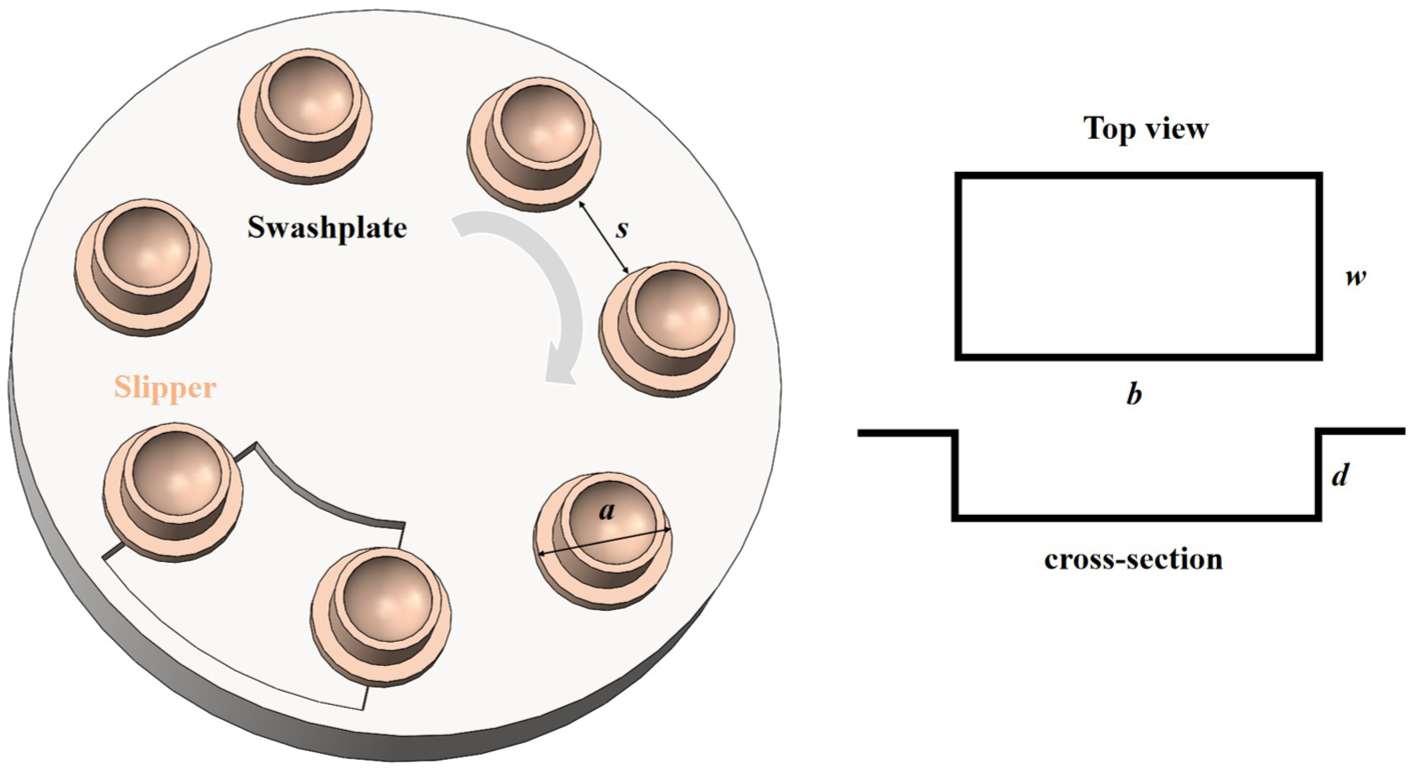
Simplified schematic diagram of the slipper and the defective swash plate.

When b > a and w > a, the motion process is shown in Figure 2. The contact between the slipper and the defect is divided into three stages: when the slider approaches the defect, it triggers a half-sine rising-edge excitation; when it is in full contact with the bottom of the defect, it generates the maximum excitation; then, as it leaves the defect, it causes a half-sine falling-edge excitation. The piecewise sine function is selected to simulate H(j) based on contact mechanics: the slipper undergoes smooth elastic deformation during contact, buffered by the oil film between the slipper and swash plate. Its continuous curvature matches the gradual variation of displacement/force in practice, whereas square waves and triangular waves cannot reflect this elastic-buffering effect. As shown in Figure 2, the time-varying displacement excitation H(j) caused by the fault is defined using a piecewise formula of a half-sine function.

$$H(j)=\{\begin{array}{cc}d·\sin [\frac{\pi }{2t_1}·(\mathrm{mod}(t,T)-t_j)]\hfill & t_j\le t\le t_1+t_j\hfill \\ \multicolumn{1}{c}{d}& t_1+t_j<t<t_1+t_j\hfill \\ \multicolumn{1}{c}{d·\sin [\frac{\pi }{2t_1}·(\mathrm{mod}(t,T)-t_2-t_j)+\frac{\pi }{2}]}& t_2+t_j\le t\le t_3+t_j\hfill \\ \multicolumn{1}{c}{0}& \mathrm{else}\hfill \end{array}$$

(1)

Figure 2.

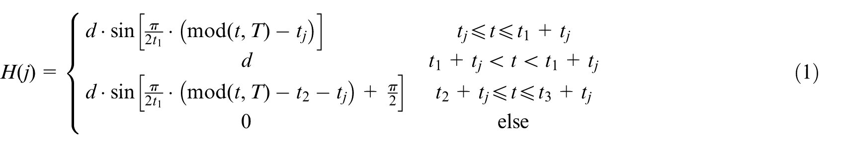
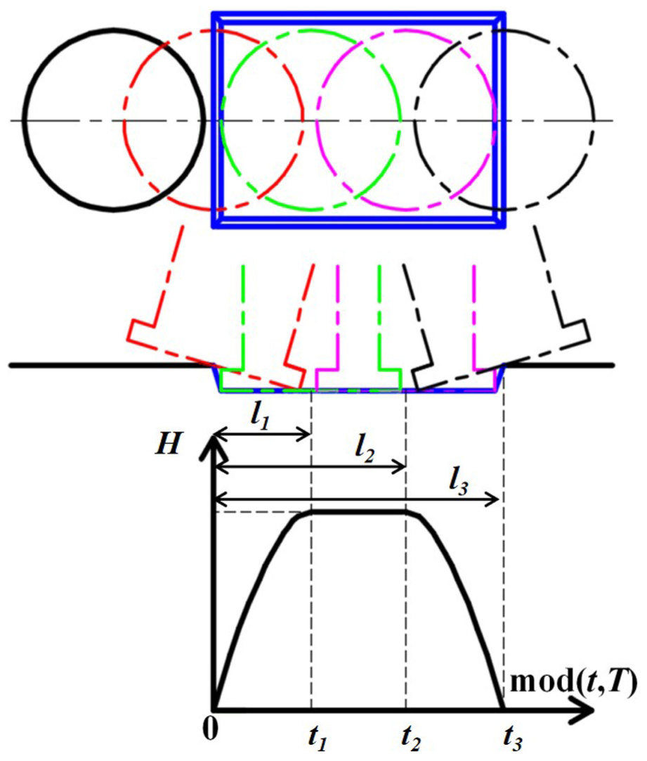
The time-varying displacement excitation H caused by the defect.

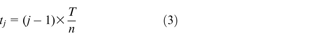
In the formula, T represents the motion period. By means of the remainder function Mod(t, T), the relative position of the time t within the motion period T can be accurately determined, so as to precisely define the time nodes corresponding to the excitation changes in different stages during the contact process between the slider and the swash plate defect. Among them, t_i(i = 1, 2, 3) and the time difference t_j(j = 1…n) between the j-th slipper’s entry into the defect and the first slipper’s entry into the defect can be expressed as follows:

$$t_i=T\times \frac{l_i}{n\times (a+s)}$$

(2)

$$t_j=(j-1)\times \frac{T}{n}$$

(3)

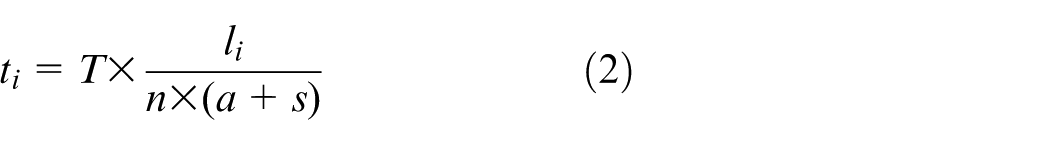
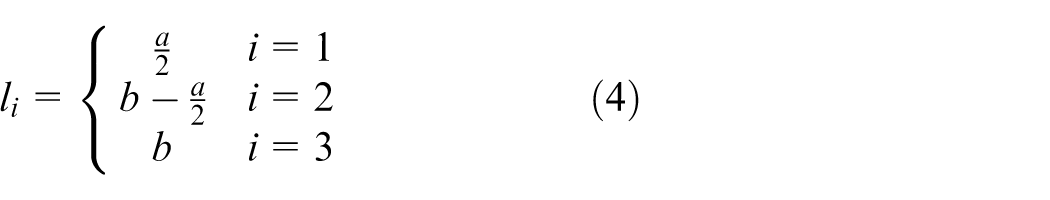
In the formula, n is the number of slippers, and l_i(i = 1, 2, 3) is the distance between the center of the slipper and the entrance edge of the defect. The expression for l _i is:

$$l_i=\{\begin{array}{cc}\frac{a}{2}\hfill & i=1\hfill \\ \multicolumn{1}{c}{b-\frac{a}{2}}& i=2\hfill \\ \multicolumn{1}{c}{b}& i=3\hfill \end{array}$$

(4)

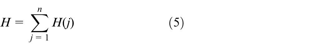
According to the above content, the total displacement excitation of n slippers is:

$$H=\sum _{j=1}^{n}H(j)$$

(5)

A dynamic model of the axial piston pump with a swash plate defect is established. As illustrated in Figure 3, the model adopts a three-mass-block configuration with 13 degrees of freedom. The pump structure is categorized into three main assemblies: the shell assembly (comprising the housing, swash plate, and valve plate), the rotor assembly (including the transmission shaft, cylinder block, pistons, and three bearings), and the remaining components (consisting of the pressure plate and spring). To simplify the dynamic modeling, the following assumptions are adopted:

• (1) The contact interfaces between the slippers and the swash plate, the valve plate and the cylinder block, and the pistons and the cylinder block are modeled as massless spring and damper elements.

• (2) The rotational motions of the pistons and slippers are neglected, and gyroscopic effects arising from rotating components are disregarded.

• (3) The housing, rotor, and remaining structural components are treated as rigid bodies.

Figure 3.

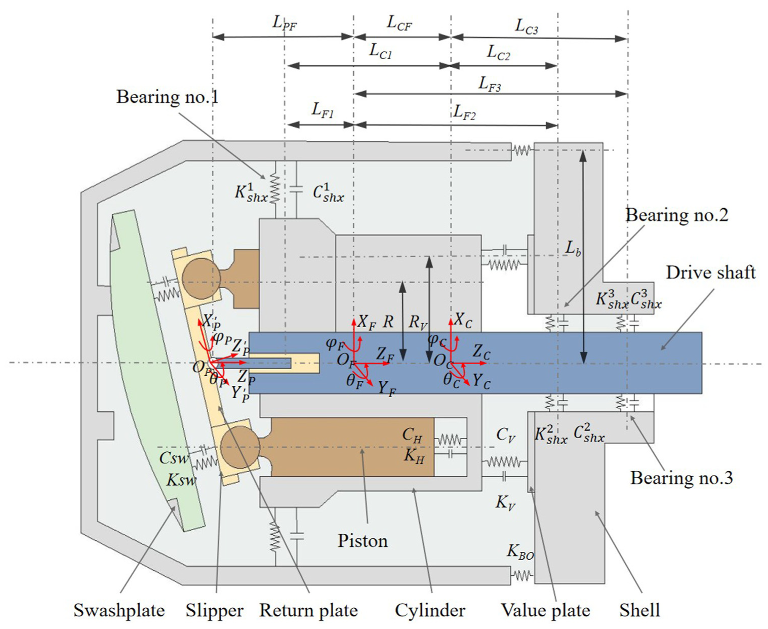
Structural schematic diagram of dynamic model of axial piston pump.

Based on these simplifications, the governing equations of motion can be derived as follows.

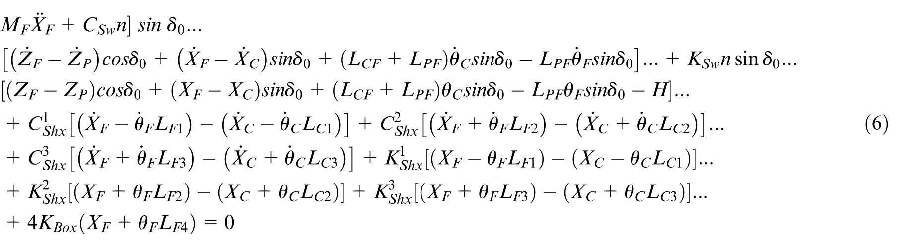
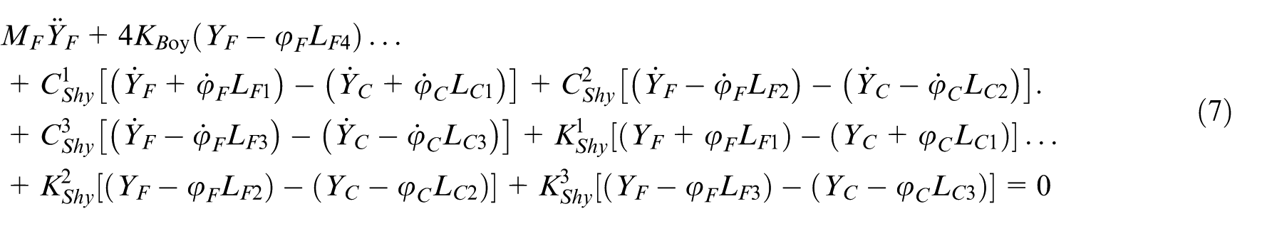
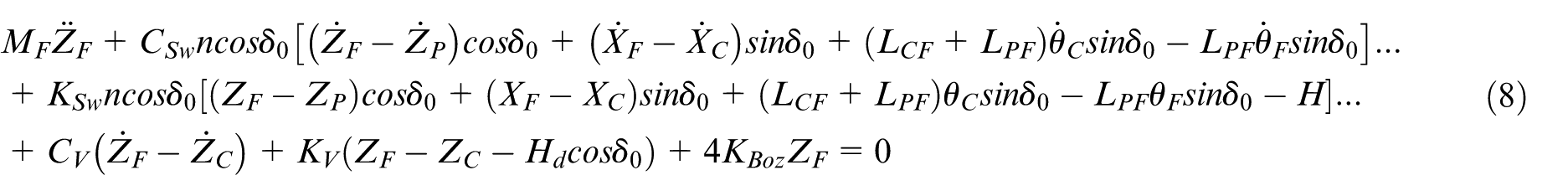
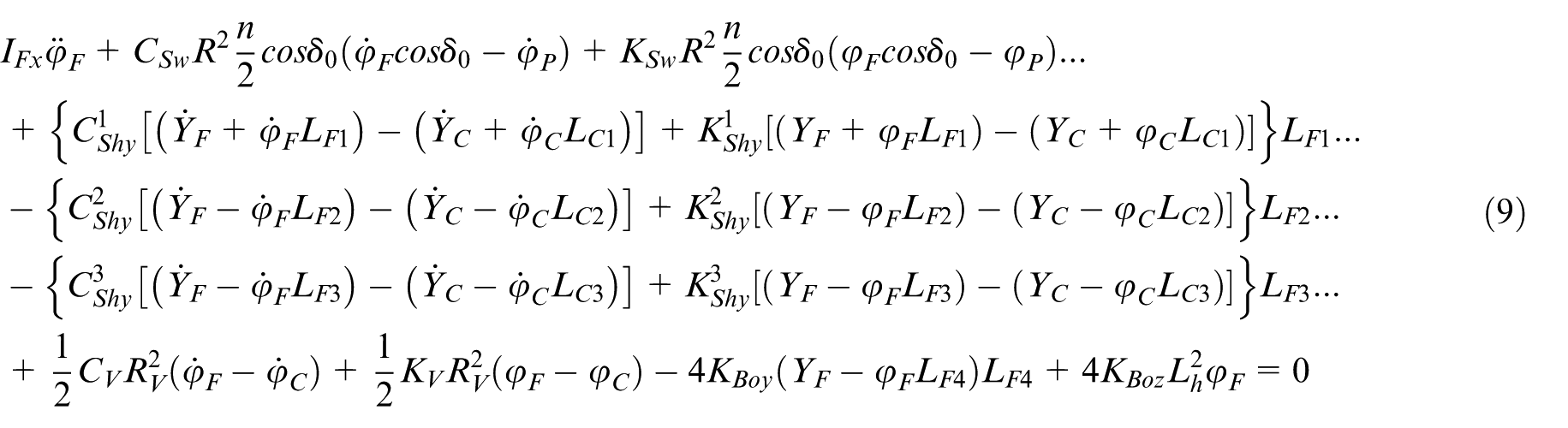
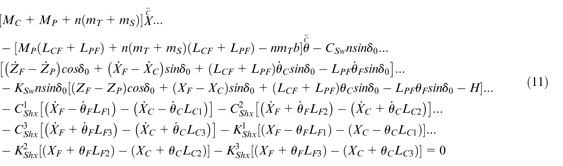
The translational motion equations of the shell assembly along the X _F , Y _F , and Z _F axes, and the rotational motion equations along the X _F and Y _F axes:

$$\begin{array}{c}{M}_F{\stackrel{··}{X}}_F+C_{\mathrm{Sw}}n]\sin {\delta }_0...\hfill \\ [({\stackrel{·}{Z}}_F-{\stackrel{·}{Z}}_P)\cos {\delta }_0+({\stackrel{·}{X}}_F-{\stackrel{·}{X}}_C)\sin {\delta }_0+(L_{\mathrm{CF}}+L_{\mathrm{PF}}){\stackrel{·}{\theta }}_C\sin {\delta }_0-L_{\mathrm{PF}}{\stackrel{·}{\theta }}_F\sin {\delta }_0]...+K_{\mathrm{Sw}}n\sin {\delta }_0...\hfill \\ [(Z_F-Z_P)\cos {\delta }_0+(X_F-X_C)\sin {\delta }_0+(L_{\mathrm{CF}}+L_{\mathrm{PF}}){\theta }_C\sin {\delta }_0-L_{\mathrm{PF}}{\theta }_F\sin {\delta }_0-H]...\hfill \\ +C_{\mathrm{Shx}}^1[({\stackrel{·}{X}}_F-{\stackrel{·}{\theta }}_F{L}_{F1})-({\stackrel{·}{X}}_C-{\stackrel{·}{\theta }}_C{L}_{C1})]+C_{\mathrm{Shx}}^2[({\stackrel{·}{X}}_F+{\stackrel{·}{\theta }}_F{L}_{F2})-({\stackrel{·}{X}}_C+{\stackrel{·}{\theta }}_C{L}_{C2})]...\hfill \\ +C_{\mathrm{Shx}}^3[({\stackrel{·}{X}}_F+{\stackrel{·}{\theta }}_F{L}_{F3})-({\stackrel{·}{X}}_C+{\stackrel{·}{\theta }}_C{L}_{C3})]+K_{\mathrm{Shx}}^1[(X_F-{\theta }_F{L}_{F1})-(X_C-{\theta }_C{L}_{C1})]...\hfill \\ +K_{\mathrm{Shx}}^2[(X_F+{\theta }_F{L}_{F2})-(X_C+{\theta }_C{L}_{C2})]+K_{\mathrm{Shx}}^3[(X_F+{\theta }_F{L}_{F3})-(X_C+{\theta }_C{L}_{C3})]...\hfill \\ +4K_{\mathrm{Box}}(X_F+{\theta }_F{L}_{F4})=0\hfill \end{array}$$

(6)

$$\begin{array}{c}\multicolumn{1}{c}{M_F{\stackrel{··}{Y}}_F+4K_{B\mathrm{oy}}(Y_F-{\phi }_F{L}_{F4})\dots }\\ \multicolumn{1}{c}{+C_{\mathrm{Shy}}^1[({\stackrel{·}{Y}}_F+{\stackrel{·}{\phi }}_F{L}_{F1})-({\stackrel{·}{Y}}_C+{\stackrel{·}{\phi }}_C{L}_{C1})]+C_{\mathrm{Shy}}^2[({\stackrel{·}{Y}}_F-{\stackrel{·}{\phi }}_F{L}_{F2})-({\stackrel{·}{Y}}_C-{\stackrel{·}{\phi }}_C{L}_{C2})].}\\ \multicolumn{1}{c}{+C_{\mathrm{Shy}}^3[({\stackrel{·}{Y}}_F-{\stackrel{·}{\phi }}_F{L}_{F3})-({\stackrel{·}{Y}}_C-{\stackrel{·}{\phi }}_C{L}_{C3})]+K_{\mathrm{Shy}}^1[(Y_F+{\phi }_F{L}_{F1})-(Y_C+{\phi }_C{L}_{C1})]\dots }\\ \multicolumn{1}{c}{+K_{\mathrm{Shy}}^2[(Y_F-{\phi }_F{L}_{F2})-(Y_C-{\phi }_C{L}_{C2})]+K_{\mathrm{Shy}}^3[(Y_F-{\phi }_F{L}_{F3})-(Y_C-{\phi }_C{L}_{C3})]=0}\end{array}$$

(7)

$$\begin{array}{c}{M}_F{\stackrel{··}{Z}}_F+C_{\mathrm{Sw}}\mathrm{ncos}{\delta }_0[({\stackrel{·}{Z}}_F-{\stackrel{·}{Z}}_P)\cos {\delta }_0+({\stackrel{·}{X}}_F-{\stackrel{·}{X}}_C)\sin {\delta }_0+(L_{\mathrm{CF}}+L_{\mathrm{PF}}){\stackrel{·}{\theta }}_C\sin {\delta }_0-L_{\mathrm{PF}}{\stackrel{·}{\theta }}_F\sin {\delta }_0]...\hfill \\ +K_{\mathrm{Sw}}\mathrm{ncos}{\delta }_0[(Z_F-Z_P)\cos {\delta }_0+(X_F-X_C)\sin {\delta }_0+(L_{\mathrm{CF}}+L_{\mathrm{PF}}){\theta }_C\sin {\delta }_0-L_{\mathrm{PF}}{\theta }_F\sin {\delta }_0-H]...\hfill \\ +C_V({\stackrel{·}{Z}}_F-{\stackrel{·}{Z}}_C)+K_V(Z_F-Z_C-H_d\cos {\delta }_0)+4K_{\mathrm{Boz}}{Z}_F=0\hfill \end{array}$$

(8)

$$\begin{array}{c}{I}_{\mathrm{Fx}}{\stackrel{··}{\phi }}_F+C_{\mathrm{Sw}}{R}^2\frac{n}{2}\cos {\delta }_0({\stackrel{·}{\phi }}_F\cos {\delta }_0-{\stackrel{·}{\phi }}_P)+K_{\mathrm{Sw}}{R}^2\frac{n}{2}\cos {\delta }_0({\phi }_F\cos {\delta }_0-{\phi }_P)...\hfill \\ +\{C_{\mathrm{Shy}}^1[({\stackrel{·}{Y}}_F+{\stackrel{·}{\phi }}_F{L}_{F1})-({\stackrel{·}{Y}}_C+{\stackrel{·}{\phi }}_C{L}_{C1})]+K_{\mathrm{Shy}}^1[(Y_F+{\phi }_F{L}_{F1})-(Y_C+{\phi }_C{L}_{C1})]\}{L}_{F1}...\hfill \\ -\{C_{\mathrm{Shy}}^2[({\stackrel{·}{Y}}_F-{\stackrel{·}{\phi }}_F{L}_{F2})-({\stackrel{·}{Y}}_C-{\stackrel{·}{\phi }}_C{L}_{C2})]+K_{\mathrm{Shy}}^2[(Y_F-{\phi }_F{L}_{F2})-(Y_C-{\phi }_C{L}_{C2})]\}{L}_{F2}...\hfill \\ -\{C_{\mathrm{Shy}}^3[({\stackrel{·}{Y}}_F-{\stackrel{·}{\phi }}_F{L}_{F3})-({\stackrel{·}{Y}}_C-{\stackrel{·}{\phi }}_C{L}_{C3})]+K_{\mathrm{Shy}}^3[(Y_F-{\phi }_F{L}_{F3})-(Y_C-{\phi }_C{L}_{C3})]\}{L}_{F3}...\hfill \\ +\frac{1}{2}{C}_V{R}_V^2({\stackrel{·}{\phi }}_F-{\stackrel{·}{\phi }}_C)+\frac{1}{2}{K}_V{R}_V^2({\phi }_F-{\phi }_C)-4K_{\mathrm{Boy}}(Y_F-{\phi }_F{L}_{F4})L_{F4}+4K_{\mathrm{Boz}}{L}_h^2{\phi }_F=0\hfill \end{array}$$

(9)

$$\begin{array}{c}{I}_{\mathrm{Fy}}{\stackrel{··}{\theta }}_F-C_{\mathrm{Sw}}{L}_{\mathrm{PF}}n\sin {\delta }_0\hfill \\ [({\stackrel{·}{Z}}_F-{\stackrel{·}{Z}}_P)\cos {\delta }_0+({\stackrel{·}{X}}_F-{\stackrel{·}{X}}_C)\sin {\delta }_0+(L_{\mathrm{CF}}+L_{\mathrm{PF}}){\stackrel{·}{\theta }}_C\sin {\delta }_0-L_{\mathrm{PF}}{\stackrel{·}{\theta }}_F\sin {\delta }_0]...\hfill \\ -K_{\mathrm{Sw}}{L}_{\mathrm{PF}}n\sin {\delta }_0\hfill \\ [(Z_F-Z_P)\cos {\delta }_0+(X_F-X_C)\sin {\delta }_0+(L_{\mathrm{CF}}+L_{\mathrm{PF}}){\theta }_C\sin {\delta }_0-L_{\mathrm{PF}}{\theta }_F\sin {\delta }_0-H]...\hfill \\ +C_{\mathrm{Sw}}\frac{n}{2}\frac{R^2}{{\cos }^2{\delta }_0}({\stackrel{·}{\theta }}_F-{\stackrel{·}{\theta }}_P)+K_{\mathrm{Sw}}\frac{n}{2}\frac{R^2}{{\cos }^2{\delta }_0}({\theta }_F-{\theta }_P)...\hfill \\ -C_{\mathrm{Shx}}^1[({\stackrel{·}{X}}_F-{\stackrel{·}{\theta }}_F{L}_{F1})-({\stackrel{·}{X}}_C-{\stackrel{·}{\theta }}_C{L}_{C1})]L_{F1}+C_{\mathrm{Shx}}^2[({\stackrel{·}{X}}_F+{\stackrel{·}{\theta }}_F{L}_{F2})-({\stackrel{·}{X}}_C+{\stackrel{·}{\theta }}_C{L}_{C2})]L_{F2}...\hfill \\ +C_{\mathrm{Shx}}^3[({\stackrel{·}{X}}_F+{\stackrel{·}{\theta }}_F{L}_{F3})-({\stackrel{·}{X}}_C+{\stackrel{·}{\theta }}_C{L}_{C3})]L_{F3}-K_{\mathrm{Shx}}^1[(X_F-{\theta }_F{L}_{F1})-(X_C-{\theta }_C{L}_{C1})]L_{F1}...\hfill \\ +K_{\mathrm{Shx}}^2[(X_F+{\theta }_F{L}_{F2})-(X_C+{\theta }_C{L}_{C2})]L_{F2}+K_{\mathrm{Shx}}^3[(X_F+{\theta }_F{L}_{F3})-(X_C+{\theta }_C{L}_{C3})]L_{F3}...\hfill \\ +\frac{1}{2}{C}_V{R}_V^2({\stackrel{·}{\theta }}_F-{\stackrel{·}{\theta }}_C)+\frac{1}{2}{K}_V{R}_V^2({\theta }_F-{\theta }_C)+4K_{\mathrm{Box}}(X_F+{\theta }_F{L}_{F4})L_{F4}+4K_{\mathrm{Boz}}{L}_b^2{\theta }_F=0\hfill \end{array}$$

(10)

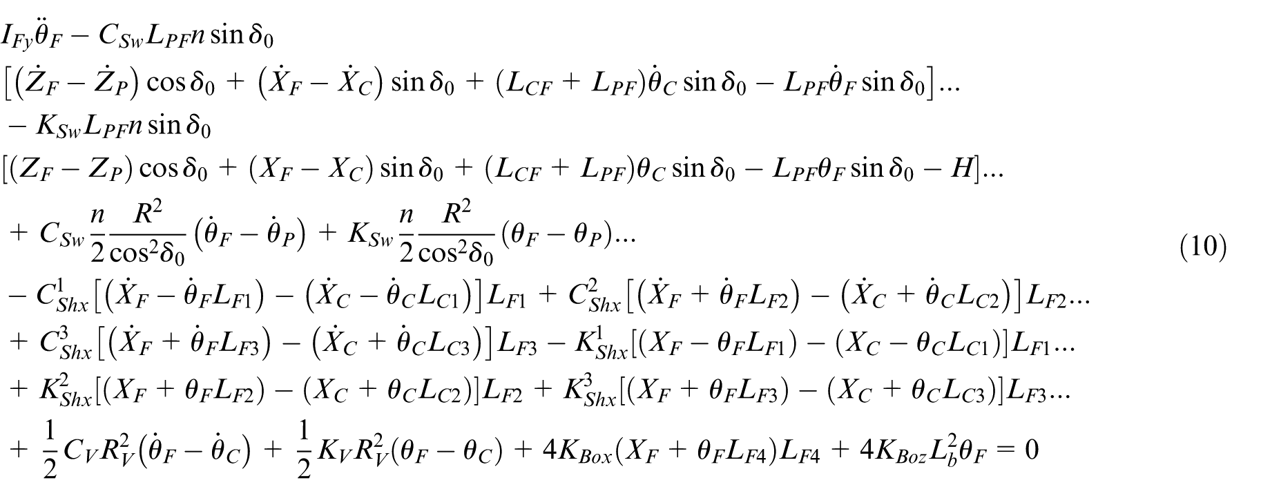
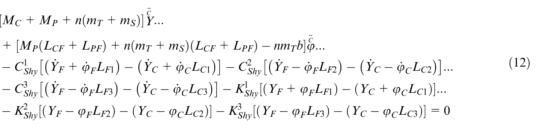
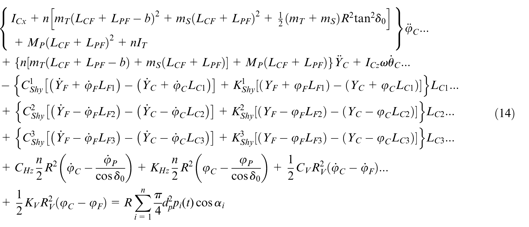
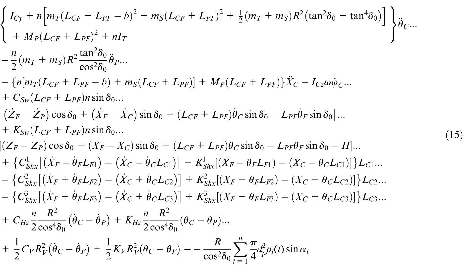
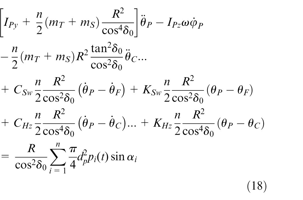
The translational motion equations of the rotor assembly along the X _C , Y _C , and Z _C axes, and the rotational motion equations along the X _C and Y _C axes:

$$\begin{array}{c}[M_C+M_P+n(m_T+m_S)]X^{\stackrel{··}{C}}...\hfill \\ -[M_P(L_{\mathrm{CF}}+L_{\mathrm{PF}})+n(m_T+m_S)(L_{\mathrm{CF}}+L_{\mathrm{PF}})-n{m}_{T}b]{\theta }^{\stackrel{··}{C}}-C_{\mathrm{Sw}}\mathrm{nsin}{\delta }_0...\hfill \\ [({\stackrel{·}{Z}}_F-{\stackrel{·}{Z}}_P)\cos {\delta }_0+({\stackrel{·}{X}}_F-{\stackrel{·}{X}}_C)\sin {\delta }_0+(L_{\mathrm{CF}}+L_{\mathrm{PF}}){\stackrel{·}{\theta }}_C\sin {\delta }_0-L_{\mathrm{PF}}{\stackrel{·}{\theta }}_F\sin {\delta }_0]...\hfill \\ -K_{\mathrm{Sw}}\mathrm{nsin}{\delta }_0[(Z_F-Z_P)\cos {\delta }_0+(X_F-X_C)\sin {\delta }_0+(L_{\mathrm{CF}}+L_{\mathrm{PF}}){\theta }_C\sin {\delta }_0-L_{\mathrm{PF}}{\theta }_F\sin {\delta }_0-H]...\hfill \\ -C_{\mathrm{Shx}}^1[({\stackrel{·}{X}}_F-{\stackrel{·}{\theta }}_F{L}_{F1})-({\stackrel{·}{X}}_C-{\stackrel{·}{\theta }}_C{L}_{C1})]-C_{\mathrm{Shx}}^2[({\stackrel{·}{X}}_F+{\stackrel{·}{\theta }}_F{L}_{F2})-({\stackrel{·}{X}}_C+{\stackrel{·}{\theta }}_C{L}_{C2})]...\hfill \\ -C_{\mathrm{Shx}}^3[({\stackrel{·}{X}}_F+{\stackrel{·}{\theta }}_F{L}_{F3})-({\stackrel{·}{X}}_C+{\stackrel{·}{\theta }}_C{L}_{C3})]-K_{\mathrm{Shx}}^1[(X_F-{\theta }_F{L}_{F1})-(X_C-{\theta }_C{L}_{C1})]...\hfill \\ -K_{\mathrm{Shx}}^2[(X_F+{\theta }_F{L}_{F2})-(X_C+{\theta }_C{L}_{C2})]-K_{\mathrm{Shx}}^3[(X_F+{\theta }_F{L}_{F3})-(X_C+{\theta }_C{L}_{C3})]=0\hfill \end{array}$$

(11)

$$\begin{array}{c}[M_C+M_P+n(m_T+m_S)]Y^{\stackrel{··}{C}}...\hfill \\ +[M_P(L_{\mathrm{CF}}+L_{\mathrm{PF}})+n(m_T+m_S)(L_{\mathrm{CF}}+L_{\mathrm{PF}})-n{m}_{T}b]{\phi }^{\stackrel{··}{C}}...\hfill \\ -C_{\mathrm{Shy}}^1[({\stackrel{·}{Y}}_F+{\stackrel{·}{\phi }}_F{L}_{F1})-({\stackrel{·}{Y}}_C+{\stackrel{·}{\phi }}_C{L}_{C1})]-C_{\mathrm{Shy}}^2[({\stackrel{·}{Y}}_F-{\stackrel{·}{\phi }}_F{L}_{F2})-({\stackrel{·}{Y}}_C-{\stackrel{·}{\phi }}_C{L}_{C2})]...\hfill \\ -C_{\mathrm{Shy}}^3[({\stackrel{·}{Y}}_F-{\stackrel{·}{\phi }}_F{L}_{F3})-({\stackrel{·}{Y}}_C-{\stackrel{·}{\phi }}_C{L}_{C3})]-K_{\mathrm{Shy}}^1[(Y_F+{\phi }_F{L}_{F1})-(Y_C+{\phi }_C{L}_{C1})]...\hfill \\ -K_{\mathrm{Shy}}^2[(Y_F-{\phi }_F{L}_{F2})-(Y_C-{\phi }_C{L}_{C2})]-K_{\mathrm{Shy}}^3[(Y_F-{\phi }_F{L}_{F3})-(Y_C-{\phi }_C{L}_{C3})]=0\hfill \end{array}$$

(12)

$$\begin{array}{c}{M}_C{\stackrel{··}{Z}}_C+C_{\mathrm{Hz}}n({\stackrel{·}{Z}}_C-{\stackrel{·}{Z}}_P)+K_{\mathrm{Hz}}n(Z_C-Z_P)+C_V({\stackrel{·}{Z}}_C-{\stackrel{·}{Z}}_F)...\hfill \\ +K_V(Z_C-Z_F+H_d\cos {\delta }_0)+K_P(Z_C-Z_P+H_d\cos {\delta }_0)=\sum _{i=1}^n\frac{\pi }{4}{d}_p^2{p}_i(t)\hfill \end{array}$$

(13)

$$\begin{array}{c}\left\{\begin{array}{c}{I}_{\mathrm{Cx}}+n[m_T{(L_{\mathrm{CF}}+L_{\mathrm{PF}}-b)}^2+m_S{(L_{\mathrm{CF}}+L_{\mathrm{PF}})}^2+\frac{1}{2}(m_T+m_S)R^2{\tan }^2{\delta }_0]\hfill \\ \multicolumn{1}{c}{+M_P{(L_{\mathrm{CF}}+L_{\mathrm{PF}})}^2+n{I}_T}\end{array}\right\}{\stackrel{··}{\phi }}_C...\hfill \\ +\{n[m_T(L_{\mathrm{CF}}+L_{\mathrm{PF}}-b)+m_S(L_{\mathrm{CF}}+L_{\mathrm{PF}})]+M_P(L_{\mathrm{CF}}+L_{\mathrm{PF}})\}{\stackrel{··}{Y}}_C+I_{\mathrm{Cz}}\omega {\stackrel{·}{\theta }}_C...\hfill \\ -\{C_{\mathrm{Shy}}^1[({\stackrel{·}{Y}}_F+{\stackrel{·}{\phi }}_F{L}_{F1})-({\stackrel{·}{Y}}_C+{\stackrel{·}{\phi }}_C{L}_{C1})]+K_{\mathrm{Shy}}^1[(Y_F+{\phi }_F{L}_{F1})-(Y_C+{\phi }_C{L}_{C1})]\}{L}_{C1}...\hfill \\ +\{C_{\mathrm{Shy}}^2[({\stackrel{·}{Y}}_F-{\stackrel{·}{\phi }}_F{L}_{F2})-({\stackrel{·}{Y}}_C-{\stackrel{·}{\phi }}_C{L}_{C2})]+K_{\mathrm{Shy}}^2[(Y_F-{\phi }_F{L}_{F2})-(Y_C-{\phi }_C{L}_{C2})]\}{L}_{C2}...\hfill \\ +\{C_{\mathrm{Shy}}^3[({\stackrel{·}{Y}}_F-{\stackrel{·}{\phi }}_F{L}_{F3})-({\stackrel{·}{Y}}_C-{\stackrel{·}{\phi }}_C{L}_{C3})]+K_{\mathrm{Shy}}^3[(Y_F-{\phi }_F{L}_{F3})-(Y_C-{\phi }_C{L}_{C3})]\}{L}_{C3}...\hfill \\ +C_{\mathrm{Hz}}\frac{n}{2}{R}^2({\stackrel{·}{\phi }}_C-\frac{{\stackrel{·}{\phi }}_P}{\cos {\delta }_0})+K_{\mathrm{Hz}}\frac{n}{2}{R}^2({\phi }_C-\frac{{\phi }_P}{\cos {\delta }_0})+\frac{1}{2}{C}_V{R}_V^2({\stackrel{·}{\phi }}_C-{\stackrel{·}{\phi }}_F)...\hfill \\ +\frac{1}{2}{K}_V{R}_V^2({\phi }_C-{\phi }_F)=R\sum _{i=1}^n\frac{\pi }{4}{d}_p^2{p}_i(t)\cos {\alpha }_i\hfill \end{array}$$

(14)

$$\begin{array}{l}\left\{I_{Cy}+n\left[m_T{\left(L_{CF}+L_{PF}-b\right)}^2+m_S{\left(L_{CF}+L_{PF}\right)}^2+\frac{1}{2}\left(m_T+m_S\right)R^2\left({\tan }^2{\delta }_0+{\tan }^4{\delta }_0\right)\right]+M_P{\left(L_{CF}+L_{PF}\right)}^2+n{I}_T\right\}{\stackrel{··}{\theta }}_C\dots \\ -\frac{n}{2}\left(m_T+m_S\right)R^2\frac{{\tan }^2{\delta }_0}{{\cos }^2{\delta }_0}{\stackrel{··}{\theta }}_P\dots -\left\{n\left[m_T\left(L_{CF}+L_{PF}-b\right)+m_S\left(L_{CF}+L_{PF}\right)\right]+M_P\left(L_{CF}+L_{PF}\right)\right\}{\stackrel{··}{X}}_C-I_{Cz}\omega {\stackrel{·}{\phi }}_C\dots \\ +C_{Sw}\left(L_{CF}+L_{PF}\right)n\sin {\delta }_0\dots \left[\left({\stackrel{·}{Z}}_F-{\stackrel{·}{Z}}_P\right)\cos {\delta }_0+\left({\stackrel{·}{X}}_F-{\stackrel{·}{X}}_C\right)\sin {\delta }_0+\left(L_{CF}+L_{PF}\right){\stackrel{·}{\theta }}_C\sin {\delta }_0-L_{PF}{\stackrel{·}{\theta }}_F\sin {\delta }_0\right]\dots +K_{Sw}\left(L_{CF}+L_{PF}\right)n\sin {\delta }_0\dots \\ \left[\left(Z_F-Z_P\right)\cos {\delta }_0+\left(X_F-X_C\right)\sin {\delta }_0+\left(L_{CF}+L_{PF}\right){\theta }_C\sin {\delta }_0-L_{PF}{\theta }_F\sin {\delta }_0-H\right]\dots \\ +\left\{C_{Shx}^1\left[\left({\stackrel{·}{X}}_F-{\stackrel{·}{\theta }}_F{L}_{F1}\right)-\left({\stackrel{·}{X}}_C-{\stackrel{·}{\theta }}_C{L}_{C1}\right)\right]+K_{Shx}^1\left[\left(X_F-{\theta }_F{L}_{F1}\right)-\left(X_C-{\theta }_C{L}_{C1}\right)\right]\right\}{L}_{C1}\dots \\ -\left\{C_{Shx}^2\left[\left({\stackrel{·}{X}}_F+{\stackrel{·}{\theta }}_F{L}_{F2}\right)-\left({\stackrel{·}{X}}_C+{\stackrel{·}{\theta }}_C{L}_{C2}\right)\right]+K_{Shx}^2\left[\left(X_F+{\theta }_F{L}_{F2}\right)-\left(X_C+{\theta }_C{L}_{C2}\right)\right]\right\}{L}_{C2}\dots \\ \left\{C_{Shx}^3\left[\left({\stackrel{·}{X}}_F+{\stackrel{·}{\theta }}_F{L}_{F3}\right)-\left({\stackrel{·}{X}}_C+{\stackrel{·}{\theta }}_C{L}_{C3}\right)\right]+K_{Shx}^3\left[\left(X_F+{\theta }_F{L}_{F3}\right)-\left(X_C+{\theta }_C{L}_{C3}\right)\right]\right\}{L}_{C3}\dots \\ +C_{Hz}\frac{n}{2}\frac{R^2}{{\cos }^4{\delta }_0}\left({\stackrel{·}{\theta }}_C-{\stackrel{·}{\theta }}_P\right)+K_{Hz}\frac{n}{2}\frac{R^2}{{\cos }^4{\delta }_0}\left({\theta }_C-{\theta }_P\right)\dots +\frac{1}{2}{C}_V{R}_V^2\left({\stackrel{·}{\theta }}_C-{\stackrel{·}{\theta }}_F\right)+\frac{1}{2}{K}_V{R}_V^2\left({\theta }_C-{\theta }_F\right)=-\frac{R}{{\cos }^2{\delta }_0}\sum _{i=1}^n\frac{\pi }{4}{d}_p^2{p}_i(t)\sin {\alpha }_i\end{array}$$

(15)

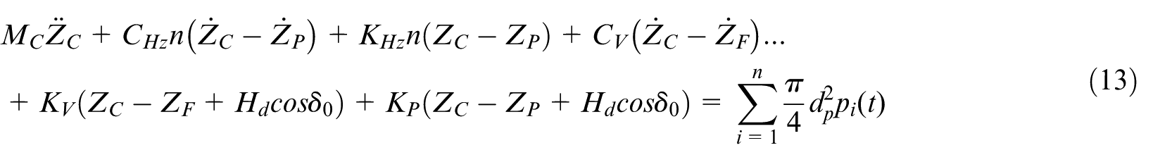
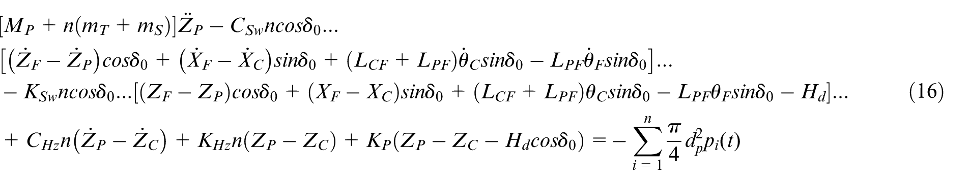
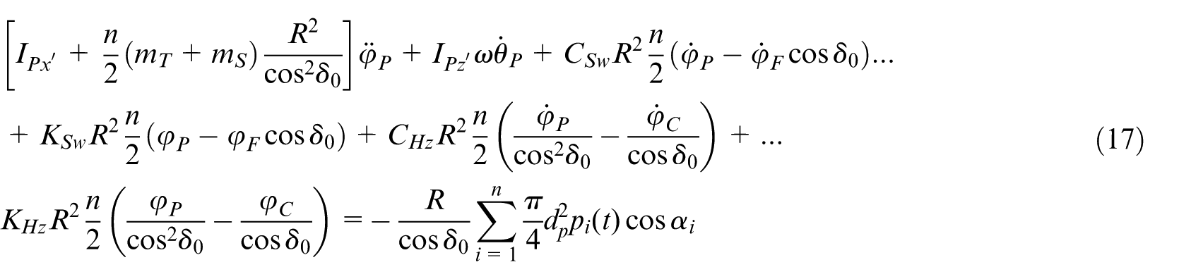
The translational motion equations of the remaining components along the Z _P axis, and the translational motion equations along the X_P′ and Y _{P ′} axes:

$$\begin{array}{c}[M_P+n(m_T+m_S)]{\stackrel{··}{Z}}_P-C_{\mathrm{Sw}}\mathrm{ncos}{\delta }_0...\hfill \\ [({\stackrel{·}{Z}}_F-{\stackrel{·}{Z}}_P)\cos {\delta }_0+({\stackrel{·}{X}}_F-{\stackrel{·}{X}}_C)\sin {\delta }_0+(L_{\mathrm{CF}}+L_{\mathrm{PF}}){\stackrel{·}{\theta }}_C\sin {\delta }_0-L_{\mathrm{PF}}{\stackrel{·}{\theta }}_F\sin {\delta }_0]...\hfill \\ -K_{\mathrm{Sw}}\mathrm{ncos}{\delta }_0...[(Z_F-Z_P)\cos {\delta }_0+(X_F-X_C)\sin {\delta }_0+(L_{\mathrm{CF}}+L_{\mathrm{PF}}){\theta }_C\sin {\delta }_0-L_{\mathrm{PF}}{\theta }_F\sin {\delta }_0-H_d]...\hfill \\ +C_{\mathrm{Hz}}n({\stackrel{·}{Z}}_P-{\stackrel{·}{Z}}_C)+K_{\mathrm{Hz}}n(Z_P-Z_C)+K_P(Z_P-Z_C-H_d\cos {\delta }_0)=-\sum _{i=1}^n\frac{\pi }{4}{d}_p^2{p}_i(t)\hfill \end{array}$$

(16)

$$\begin{array}{c}[I_{{\mathrm{Px}}^{\prime }}+\frac{n}{2}(m_T+m_S)\frac{R^2}{{\cos }^2{\delta }_0}]{\stackrel{··}{\phi }}_P+I_{{\mathrm{Pz}}^{\prime }}\omega {\stackrel{·}{\theta }}_P+C_{\mathrm{Sw}}{R}^2\frac{n}{2}({\stackrel{·}{\phi }}_P-{\stackrel{·}{\phi }}_F\cos {\delta }_0)...\hfill \\ +K_{\mathrm{Sw}}{R}^2\frac{n}{2}({\phi }_P-{\phi }_F\cos {\delta }_0)+C_{\mathrm{Hz}}{R}^2\frac{n}{2}(\frac{{\stackrel{·}{\phi }}_P}{{\cos }^2{\delta }_0}-\frac{{\stackrel{·}{\phi }}_C}{\cos {\delta }_0})+...\hfill \\ K_{\mathrm{Hz}}{R}^2\frac{n}{2}(\frac{{\phi }_P}{{\cos }^2{\delta }_0}-\frac{{\phi }_C}{\cos {\delta }_0})=-\frac{R}{\cos {\delta }_0}\sum _{i=1}^n\frac{\pi }{4}{d}_p^2{p}_i(t)\cos {\alpha }_i\hfill \end{array}$$

(17)

$$\begin{array}{c}[I_{\mathrm{Py}}+\frac{n}{2}(m_T+m_S)\frac{R^2}{{\cos }^4{\delta }_0}]{\stackrel{··}{\theta }}_P-I_{\mathrm{Pz}}\omega {\stackrel{·}{\phi }}_P\hfill \\ \multicolumn{1}{c}{-\frac{n}{2}(m_T+m_S)R^2\frac{{\tan }^2{\delta }_0}{{\cos }^2{\delta }_0}{\stackrel{··}{\theta }}_C...}\\ +C_{\mathrm{Sw}}\frac{n}{2}\frac{R^2}{{\cos }^2{\delta }_0}({\stackrel{·}{\theta }}_P-{\stackrel{·}{\theta }}_F)+K_{\mathrm{Sw}}\frac{n}{2}\frac{R^2}{{\cos }^2{\delta }_0}({\theta }_P-{\theta }_F)\hfill \\ \multicolumn{1}{c}{+C_{\mathrm{Hz}}\frac{n}{2}\frac{R^2}{{\cos }^4{\delta }_0}({\stackrel{·}{\theta }}_P-{\stackrel{·}{\theta }}_C)...+K_{\mathrm{Hz}}\frac{n}{2}\frac{R^2}{{\cos }^4{\delta }_0}({\theta }_P-{\theta }_C)}\\ \multicolumn{1}{c}{=\frac{R}{{\cos }^2{\delta }_0}\sum _{i=1}^n\frac{\pi }{4}{d}_p^2{p}_i(t)\sin {\alpha }_i}\end{array}$$

(18)

The dynamic equations are solved by Runge-Kutta method. For the key parameters in the equation, such as damping and stiffness, the coefficients refer to the provisions in References.^37,38 In the next chapter, we will discuss how to accurately identify the parameters through the fault vibration signal of the piston pump measured in the experiment.

Inverse physics-informed neural network

Physics-informed neural networks (PINNs) represent a cutting-edge methodology that integrates physical principles with deep learning to solve scientific and engineering problems. A PINN typically learns a mapping between spatiotemporal coordinates (e.g. time t and spatial coordinates x ) and the observed system response y using architectures such as Multilayer Perceptrons (MLPs), Residual Networks (ResNets), or Deep Operator Networks (DeepONets). PINN problems are broadly categorized into forward and inverse problems. In forward problems, the governing physical equations are fully known, and the network is trained to approximate the system’s response. Conversely, inverse problems treat the observed signals as known conditions. The network is then tasked with identifying unknown parameters within partially known governing equations by jointly minimizing a loss function that incorporates both data fidelity and physical consistency.

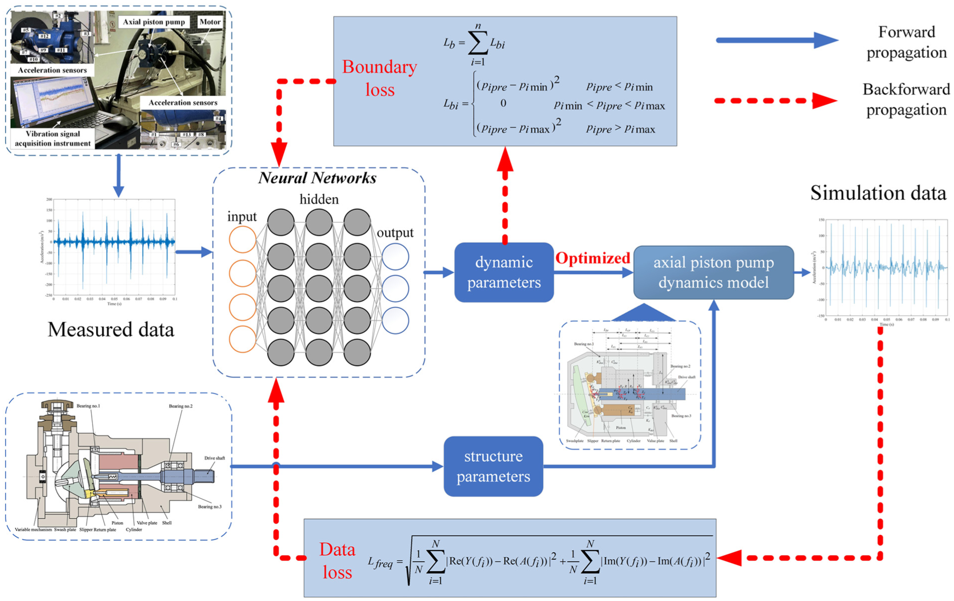
This study proposes an Inverse Physics-Informed Neural Network (IPINN), a novel architecture designed to refine the key dynamic parameters of the axial piston pump model described in Section 2.1. Unlike traditional PINNs aimed at direct response prediction, the IPINN’s objective is the inverse identification of unknown model parameters from measured vibration signals. The overall architecture of the proposed IPINN is illustrated in Figure 4.

Figure 4.

IPINN structure.

The IPINN takes the measured vibration acceleration signals of the axial piston pump as input. A multi-layer convolutional network extracts hierarchical features from these signals. A critical design innovation is implemented at the output layer. To address the significant scale disparity (spanning orders of 10⁴–10⁸) among different dynamic parameters (e.g. stiffness K _sw and damping C _sw ), which can destabilize training, a “base value × magnitude” decoupling mechanism is introduced. The output layer uses a linear activation function to generate six parameter base values, θ = [θ₁, θ₂,…, θ₆]. These base values are then reconstructed into physically meaningful dynamic parameters P = [P₁, P₂,…, P₆] using a predefined magnitude coefficient matrix S = [s₁, s₂,…, s₆], derived from engineering expertise:

$$P=\theta \odot S$$

(19)

where ⊙ denotes element-wise multiplication. During network initialization, the bias of the output layer is fixed to a preset baseline b, ensuring that the initial forward pass yields parameters within a reasonable engineering range.

The reconstructed parameters P are substituted, along with fixed structural parameters, into the axial piston pump dynamic equations established in Section 2.1. The fourth-order Runge-Kutta method is employed to numerically solve these equations, yielding simulated acceleration signals. A composite loss function enforcing both physical constraints and data fidelity guides the training:

$$\mathrm{Loss}=L_b+L_{\mathrm{freq}}$$

(20)

Where Loss is the total loss, composed of a boundary lossL _b and a data loss L _freq .

The boundary loss function ensures the physical reasonableness of optimized parameters by restricting their value ranges, guides network training using prior knowledge such as parameter upper and lower limits, accelerates the convergence process, and avoids unreasonable parameter values. The expressions of the boundary loss Lb are shown in equations (21) and (22).

$$L_{\mathrm{bi}}=\{\begin{array}{cc}{(P_{\mathrm{ipre}}-P_{\mathrm{imin}})}^2\hfill & P_{\mathrm{ipre}}<P_{\mathrm{imin}}\hfill \\ \multicolumn{1}{c}{0}& P_{\mathrm{imin}}<P_{\mathrm{ipre}}<P_{\mathrm{imax}}\hfill \\ \multicolumn{1}{c}{{(P_{\mathrm{ipre}}-P_{\mathrm{imax}})}^2}& P_{\mathrm{ipre}}>P_{\mathrm{imax}}\hfill \end{array}$$

(21)

$$L_b=\sum _{i=1}^n{L}_{\mathrm{bi}}$$

(22)

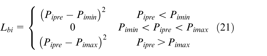
Here, P _ipre represents the j-th parameter output by the network model. P _imin and P _imax are respectively the lower and upper limits of this parameter. n is the number of parameters. The specific upper and lower limits of the parameters are set according to their value ranges, while the approximate ranges of the parameter values are determined based on the empirical knowledge related to the target object.

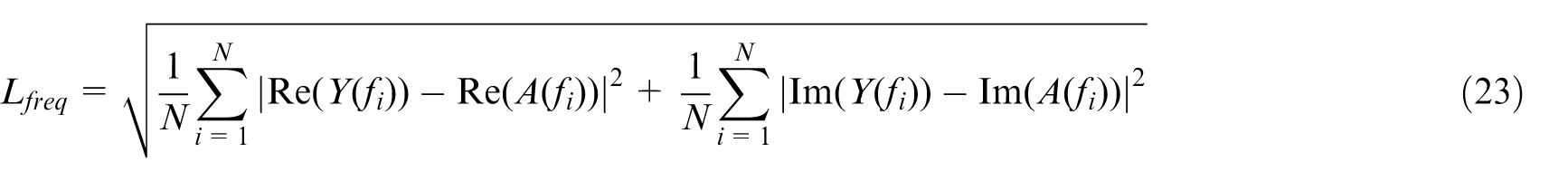
To calculate the discrepancy between the simulation and experimental data, we analyze the signals in the frequency domain. Converting the time-domain signals to the frequency domain effectively eliminates interference from factors such as phase differences while accentuating the impact of dynamic parameters on the spectrum. To ensure the optimized parameters accurately reflect the actual physical process, we employ the Root Mean Square Error (RMSE) to quantify the difference between the simulation and experimental data. The data loss is defined as shown in equation (23).

$$L_{\mathrm{freq}}=\sqrt{\frac{1}{N}\sum _{i=1}^N{|\mathrm{Re}(Y(f_i))-\mathrm{Re}(A(f_i))|}^2+\frac{1}{N}\sum _{i=1}^N{|\mathrm{Im}(Y(f_i))-\mathrm{Im}(A(f_i))|}^2}$$

(23)

Specific Steps of the Proposed IPINN

• Step 1: Feed the structural parameters of the axial piston pump into the system, and input the vibration acceleration signals collected under working conditions into the IPINN. Utilizing expert knowledge, establish the optimal value ranges for the dynamic parameters, and set those parameters to their initial values within the defined ranges.

• Step 2: Using dynamic/structural parameters, the dynamic equations of an axial piston pump with a tilted plate fault are solved via the Runge-Kutta-Tensor method to generate simulated vibration acceleration signals.

• Step 3: Calculate the Fourier transforms for both the signals that have been simulated and those that have been measured experimentally. The IPINN then calculates and outputs the dynamic parameters.

• Step 4: Use equation (23) to calculate the data loss L _freq , and use equations (21) and (22) to compute the boundary loss L _b .

• Step 5: Use Adam Optimizer to determine the total loss and train reverse IPINN. Adjust network parameters according to these losses.

• Step 6: Repeat 2–5 steps to the IPINN. After training, accurately detect dynamic parameters.

• Step 7: Optimized dynamic parameters are included in the dynamic model to generate new data from the analog signal.

The process is shown in Figure 5 demonstrates that by integrating simulated samples into the training dataset, the imbalance present in swash plate fault samples is alleviated, which enhances the accuracy of diagnosing imbalanced faults.

Figure 5.

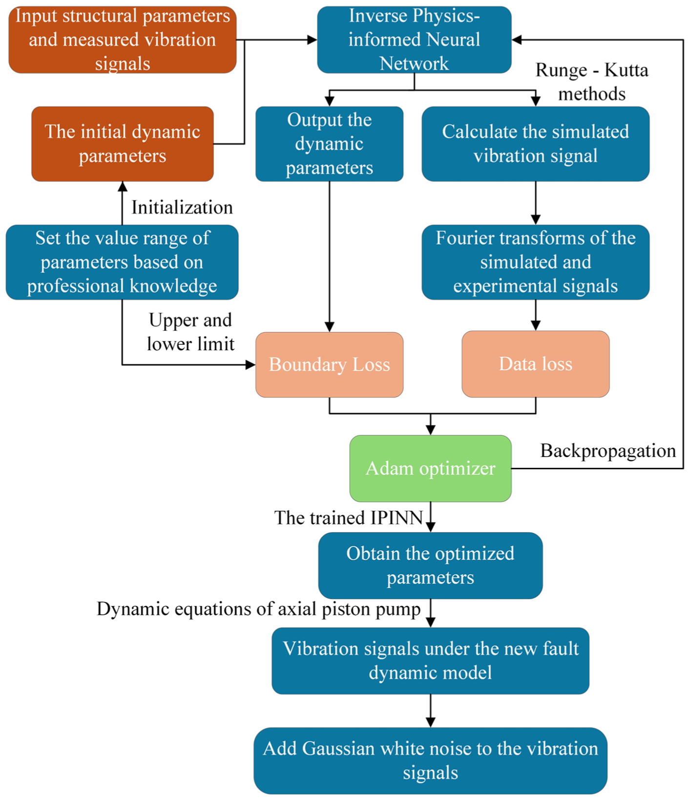
Specific steps of the fault data generation method.

Bidirectional temporal convolutional network (BiTCN)

In the field of rotating machinery fault diagnosis, the non-stationarity and multi-scale coupling characteristics of vibration signals pose significant challenges for fault feature extraction. Traditional manual feature extraction methods are not only inefficient but also struggle to adapt to complex working conditions, resulting in suboptimal diagnostic accuracy. The Bidirectional Temporal Convolutional Network (BiTCN), which integrates the advantages of bidirectional temporal dependency modeling and CNN, offers a new solution for fault diagnosis.

Residual unit structure

The residual unit serves as a fundamental building block for constructing the BiTCN, and its specific structure is illustrated in Figure 6. Its design addresses the challenges of vanishing or exploding gradients that may arise in deep networks, ensuring the stability of the network as its depth increases. Within the residual unit, the Dilated Causal Convolution operation effectively extracts features at different temporal scales without significantly increasing computational complexity by configuring parameters such as the convolution kernel size, dilation rate, and padding. Adjusting the dilation rate expands the receptive field of the convolution kernel, enabling the capture of long-range temporal dependencies in the signal, while padding ensures that the output feature dimensions remain consistent.

Figure 6.

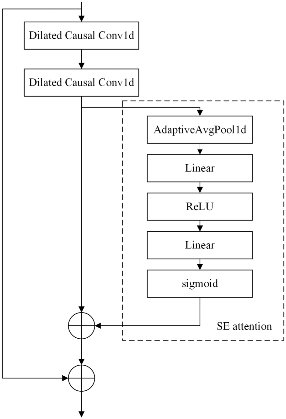
Schematic diagram of residual unit structure.

The Batch Normalization layer accelerates network convergence and mitigates internal covariate shift. The ReLU activation function introduces non-linearity, enhancing the network’s expressive power. The Dropout layer prevents overfitting by randomly disabling neurons during training. Additionally, the residual unit incorporates the Squeeze-and-Excitation (SE) attention mechanism, as shown within the dashed box in Figure 6. This mechanism globally aggregates channel-wise features through Adaptive Average Pooling to capture global information, then employs two linear layers with ReLU and Sigmoid activations to learn channel dependencies and generate channel weights. These weights are multiplied element-wise with the original feature maps to emphasize important channels and suppress irrelevant ones, enabling the network to focus on critical fault features.

Overall structure of BiTCN

Figure 7 depicts the overall architecture of the BiTCN, which primarily consists of Positive Residual Units and Inverse Residual Units. Upon entering the network, the input signal is processed in parallel by these two types of units. The Positive Residual Units process the signal in chronological order to explore the “past-to-future” development trends of faults, while the Inverse Residual Units process the time-reversed signal to capture “future-to-past” contextual information. Both units share a similar structure, comprising multiple stacked residual unit modules that progressively extract deeper fault features. In addition to dilated causal convolutions, batch normalization, ReLU activation functions, Dropout, and the SE attention mechanism, 1 × 1 convolutions are applied at both ends of these units. These 1 × 1 convolutions adjust the number of feature channels to facilitate residual connections and further integrate multi-scale features. The features processed by the forward and inverse paths are then fused through residual connections. The fused features are fed into a Fully Connected (FC) layer, which maps them to diagnostic outputs for accurate identification of rotating machinery fault types.

Figure 7.

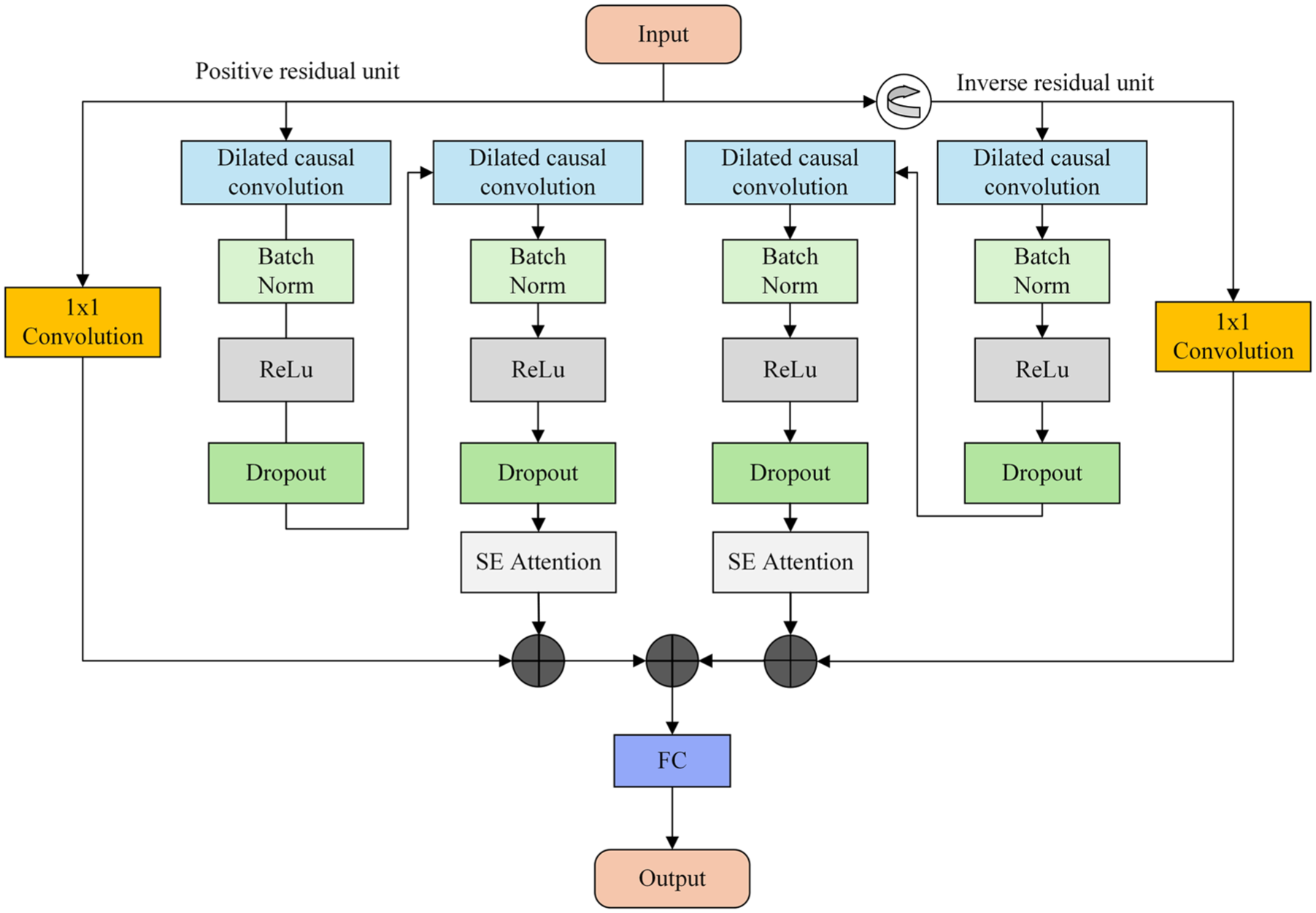
Structural diagram of BiTCN.

Experiments and analyses

Experimental description

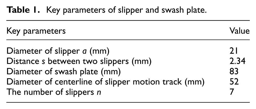
To verify the effectiveness of the proposed method, an axial piston pump test rig was built as shown in Figure 8(a). The experimental setup consists of a 25SCY14-1B type piston pump, a variable frequency motor, a relief valve, a vibration signal collector, and 13 acceleration sensors of the same model. During the experiment, the drive shaft maintains a rotational speed of 860 revolutions per minute, the suction port pressure is stabilized at 0.11 MPa, the discharge port pressure is set to 15 MPa, and the hydraulic oil temperature is controlled within the range of 30°C to 60°C. The system real-time collects and monitors key operating parameters such as shaft rotational speed, outlet pressure, outlet flow rate, and hydraulic oil temperature in the tank. The key geometric parameters of the swash plate and slippers are detailed in Table 1.

Figure 8.

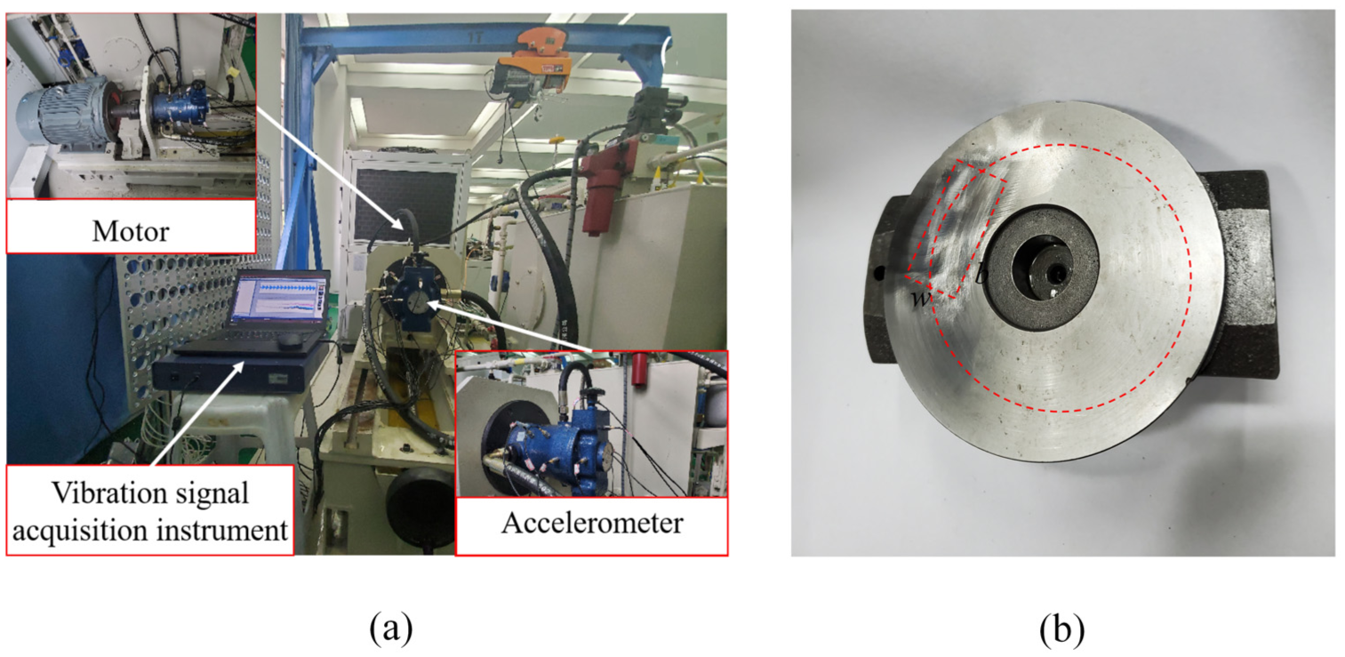
Experimental test platform: (a) experimental apparatus and (b) defective experimental swash plate.

Table 1.

Key parameters of slipper and swash plate.

Key parameters	Value
Diameter of slipper a (mm)	21
Distance s between two slippers (mm)	2.34
Diameter of swash plate (mm)	83
Diameter of centerline of slipper motion track (mm)	52
The number of slippers n	7

As shown in Figure 8(b), it is a schematic diagram of the artificially prepared defective swash plate, with its defect dimensions being: length b = 30 mm, width w = 24 mm, and depth d = 0.6 mm. Based on this physical model, the fault defect excitation function is calculated through equation (1). Figure 9 displays the displacement excitation response curves of the 7 slippers when passing through the defective area of the swash plate, while the total displacement excitation result described by equation (5) is shown in Figure 10. These experimental data provide a foundation for subsequent data augmentation and fault diagnosis algorithm verification.

Figure 9.

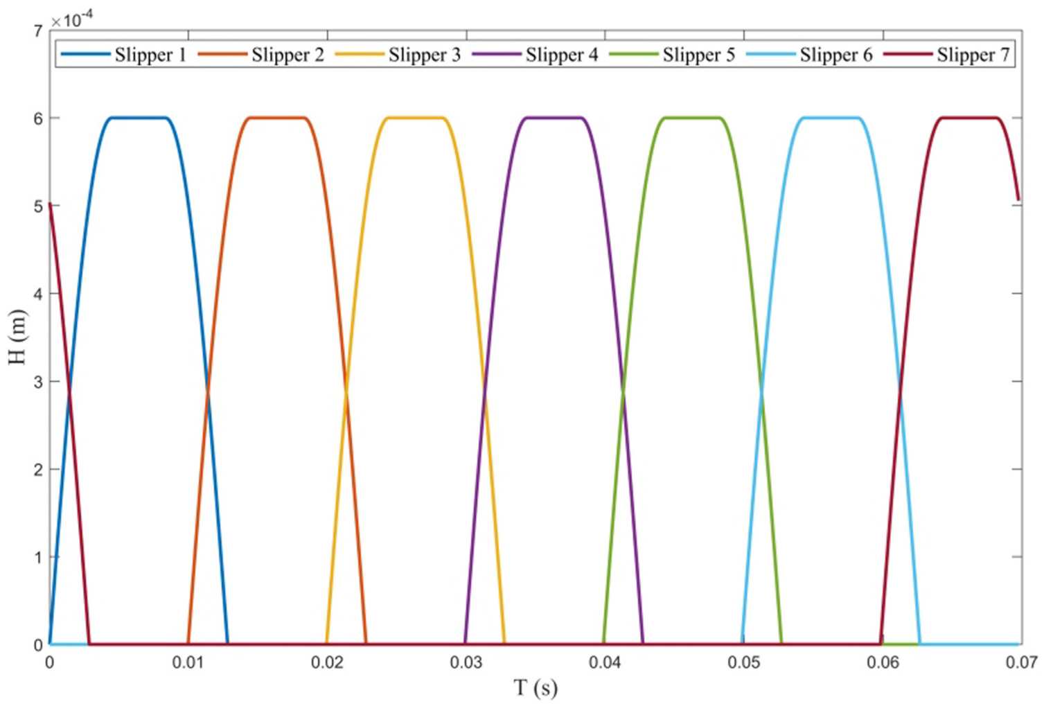
Displacement excitation response of 7 slippers passing through swash plate defect area.

Figure 10.

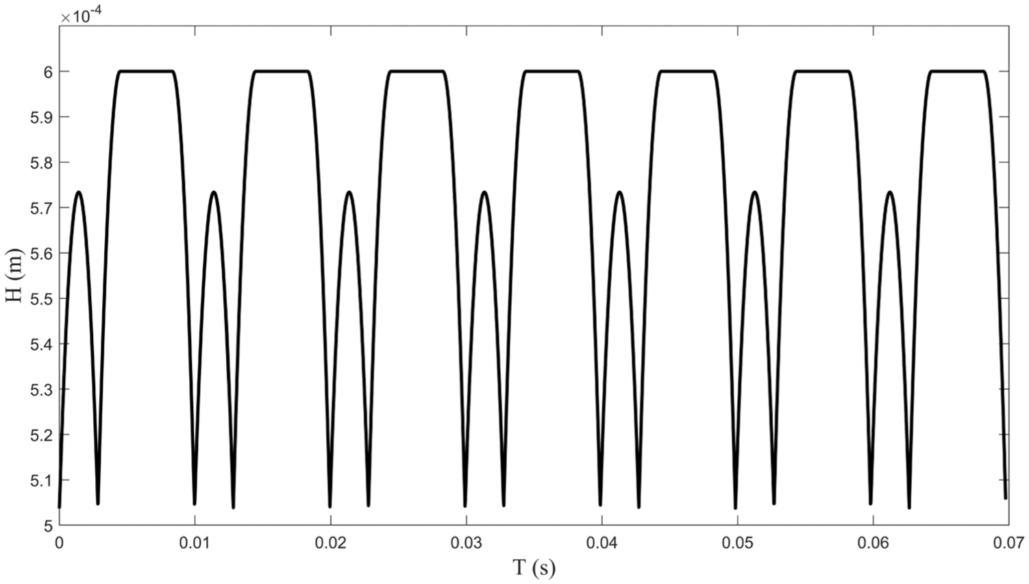
Total excitation diagram of 7 slippers.

Simulation data validation

Training details

To optimize the key dynamic parameters of the axial piston pump model, the Inverse Physics-Informed Neural Network (IPINN) was implemented with the following computational setup and hyperparameters. The training environment consisted of an Intel Core i7-12700H CPU, 16 GB RAM, and an NVIDIA GeForce RTX 4060 GPU. The software was built on Python 3.8, utilizing PyTorch and NumPy packages for network implementation and numerical computations.

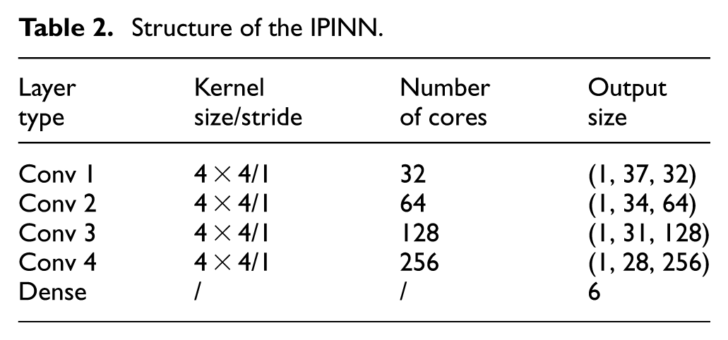
The architecture of the IPINN, detailed in Table 2, comprises a four-layer convolutional neural network (CNN) followed by a dense output layer. This structure was determined through preliminary experiments to balance model performance and complexity. The channel dimensions progressively double from 32 to 256 across the layers (32→64→128→256) to enhance feature representation capacity. The network was trained for 500 epochs using the Adam optimizer, which was selected for its stability and adaptive learning rate properties, particularly advantageous for inverse problem solving. The learning rate was set to 0.0001, optimized via a grid search over the set {0.1, 0.01, 0.001, 0.0001}. Training was monitored via loss curves to ensure convergence. These design choices, grounded in empirical tuning and established deep learning principles, ensure the reproducibility and systematic rigor of the parameter identification process.

Table 2.

Structure of the IPINN.

Layer type	Kernel size/stride	Number of cores	Output size
Conv 1	4 × 4/1	32	(1, 37, 32)
Conv 2	4 × 4/1	64	(1, 34, 64)
Conv 3	4 × 4/1	128	(1, 31, 128)
Conv 4	4 × 4/1	256	(1, 28, 256)
Dense	/	/	6

Experimental result analysis

To calibrate the dynamic model of the axial piston pump, this study employs the Inverse Physics-Informed Neural Network (IPINN) to optimize six key dynamic parameters: the damping coefficient between the slipper and the swash plate (C _sw ), the stiffness coefficient between the slipper and the swash plate (K _sw ), the cylinder damping coefficient (C _v ), the cylinder stiffness coefficient (K _Hz ), the valve plate stiffness coefficient (K _v ), and the piston damping coefficient (C _Hz ). These parameters are selected based on their central role in the dynamic model and their sensitivity to vibration responses, as they directly define the dynamic behavior of critical friction pairs such as the slipper-swash plate and piston-cylinder interfaces. After 500 training iterations, the IPINN achieved the minimum loss at the 453rd iteration, and the optimized results are summarized in Table 3.

Table 3.

The optimized dynamic parameters obtained through IPINN.

Index	Parameter	Preset baseline b	Optimized baseline θ	Magnitude S	Parameter P
1	C sw	1.86	0.778	106	7.78 × 105
2	K sw	4.32	3.58	108	3.58 × 108
3	C v	3.60	7.2	104	7.2 × 104
4	K Hz	1.20	8.2	107	8.2 × 107
5	K v	9.80	2.34	108	2.34 × 108
6	C Hz	3.40	15.3	104	1.53 × 105

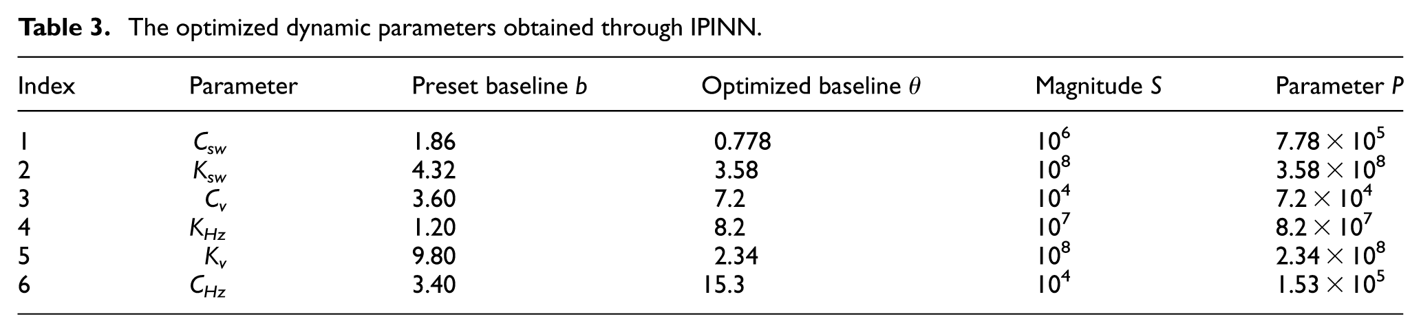
The optimized values show significant adjustments compared to the empirical baseline. For instance, C _sw decreased from 1.86 × 10⁶ N·s/m to 0.778 × 10⁶ N·s/m, while C _Hz increased from 3.40 × 10⁴ N·s/m to 15.3 × 10⁴ N·s/m. These adjustments effectively correct the systematic bias introduced by empirical estimations. All optimized parameters fall within physically plausible ranges: stiffness coefficients are on the order of 10⁷–10⁸ N/m, and damping coefficients are on the order of 10⁴–10⁵ N·s/m. This not only validates the effectiveness of the boundary loss function constraints but also demonstrates that the IPINN yields a physically self-consistent set of optimal parameters.

To evaluate the performance of the simulated signals after parameter optimization, Figure 11 compares the time-domain waveforms of vibration signals generated using empirical parameters and IPINN-optimized parameters against experimental measurements. The results indicate that the simulated signals based on optimized parameters (Figure 11(b)) exhibit high agreement with the experimental signals at key features such as peaks and troughs, and their overall fluctuation trends are more consistent. In contrast, the simulation results based on empirical parameters (Figure 11(a)) show noticeable deviations. Visual comparison confirms that the simulation accuracy is significantly improved with the optimized parameters, enabling a more accurate representation of the dynamic characteristics and variation patterns of the experimental signals.

Figure 11.

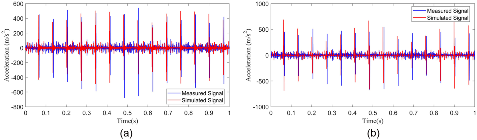
Time-domain comparison between simulation signals and experimental signals: (a) empirical simulation results and (b) simulation results after optimization.

The simulation and experimental signals were converted into spectrograms via FFT, as shown in Figure 12(a) displays the simulation spectrum derived from empirical parameters, and Figure 12(b) shows the spectrum from the optimized parameters. The optimized model also demonstrates remarkable enhancement in frequency-domain consistency with the experimental signals, especially at the fundamental frequency and its harmonics. This further validates the effectiveness of IPINN in accurately predicting the frequency characteristics of axial piston pumps.

Figure 12.

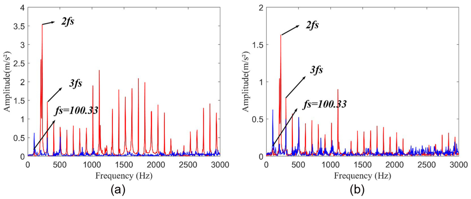
Frequency-domain comparison between the simulation signals and the experimental signals: (a) empirical simulation results and (b) simulation results after optimization.

To further verify the differences between the simulation data and the experimental data, three metrics were calculated: the Root Mean Square Error (RMSE), the Peak Error (PE), and the Spectrum Value Error (SVE). The calculation and comparison results are presented in Table 4.

Table 4.

Evaluation results of time-domain signals for different parameters.

Type of parameters	RMSE	PE	SVE
Empirical parameters	0.1054	3.6099	0.0656
Optimized parameters	0.0928	1.9833	0.0610

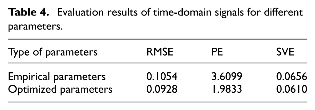
The numerical values of RMSE, PE, and SVE corresponding to the optimized parameters are all lower than those corresponding to the empirical parameters. This indicates that the simulation data obtained using the parameters optimized by IPINN have a higher degree of agreement with the experimental data, confirming the superiority of the proposed IPINN method in parameter identification and data simulation.

Application in fault diagnosis of axial piston pump

Case I: Few samples for a working condition

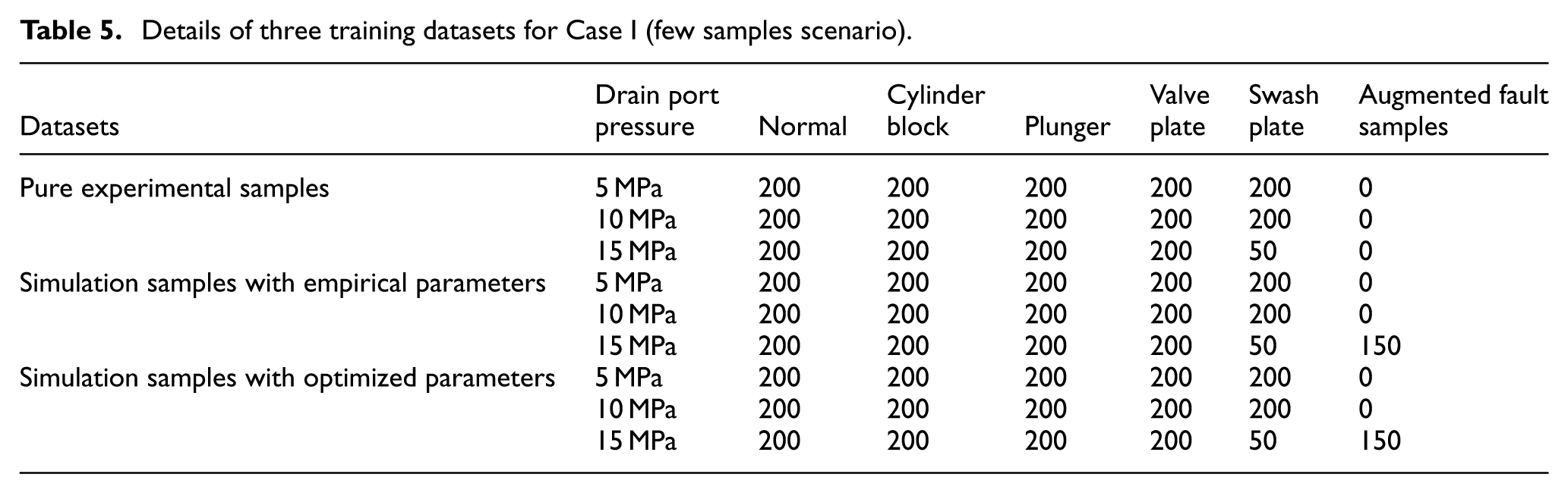
This case study was designed to validate the efficacy of the IPINN-based data augmentation method under a scenario of severe sample scarcity for a specific fault condition. The experimental data collection covered five states of the axial piston pump. While the normal state and three other fault types (cylinder block, plunger, and valve plate) each had 650 samples under three pressure conditions (5, 10, and 15 MPa), the swash plate fault was critically under-represented with only 500 total samples. The scarcity was most acute at the 15 MPa condition, where only 50 swash plate fault samples were available, creating a significant class imbalance.

To address this, simulation data was generated under the 15 MPa condition to augment the scarce swash plate fault class. Two simulation strategies were employed for comparison: one using traditional empirical parameters and the other using parameters optimized by the proposed IPINN method. Each strategy generated 150 supplementary swash plate fault samples. To validate the effectiveness of the method in extreme data-absent scenarios, this study established a condition where experimental data for the swash plate fault under 15 MPa working condition were completely missing, and constructed three comparative training datasets (see Table 5 for details): Pure Experimental Dataset (containing only measured data), Empirical-Parameter Simulation Dataset (filling the missing data with 200 simulation samples generated using traditional empirical parameters), and Optimized-Parameter Simulation Dataset (filling the missing data with 200 high-fidelity simulation samples generated using IPINN-optimized parameters). The employed BiTCN diagnostic model, with its detailed network architecture and hyperparameter configuration provided in Table 6, is designed with bidirectional dilated causal convolutions and an attention mechanism to ensure efficient extraction and classification of temporal fault features.

Table 5.

Details of three training datasets for Case I (few samples scenario).

Datasets	Drain port pressure	Normal	Cylinder block	Plunger	Valve plate	Swashplate	Augmented fault samples
Pure experimental samples	5 MPa	200	200	200	200	200	0
	10 MPa	200	200	200	200	200	0
	15 MPa	200	200	200	200	50	0
Simulation samples with empirical parameters	5 MPa	200	200	200	200	200	0
	10 MPa	200	200	200	200	200	0
	15 MPa	200	200	200	200	50	150
Simulation samples with optimized parameters	5 MPa	200	200	200	200	200	0
	10 MPa	200	200	200	200	200	0
	15 MPa	200	200	200	200	50	150

Table 6.

BiTCN network layer parameters.

Layer	Hyperparameters	Output Shape
Dilated Causal Conv1d	Kernel = 3, Stride = 1, Padding = 1, Dilation = 1	(−1, 32, 1000)
Dilated Causal Conv1d	Kernel = 3, Stride = 1, Padding = 2, Dilation = 2	(−1, 16, 1000)
SE attention	/	(−1, 16, 1)
Positive Residual Unit	/	(−1, 16, 1000)
Dilated Causal Conv1d	Kernel = 3, Stride = 1, Padding = 1, Dilation = 1	(−1, 32, 1000)
Dilated Causal Conv1d	Kernel = 3, Stride = 1, Padding = 2, Dilation = 2	(−1, 32, 1000)
SE attention	/	(−1, 16, 1)
Inverse Residual Unit	/	(−1, 16, 1000)
FC	/	(−1, 5)

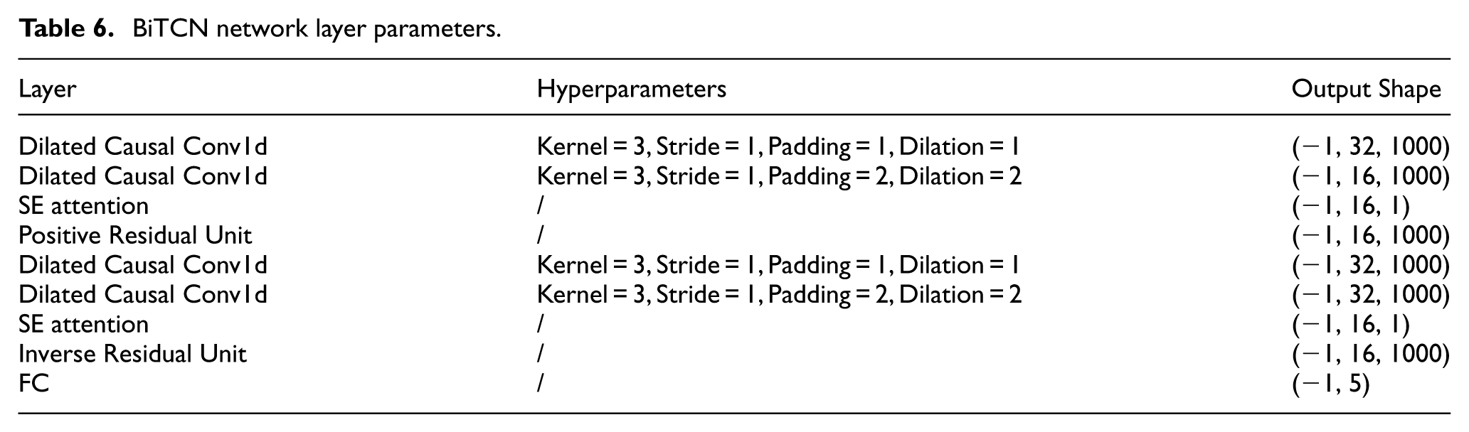
The Bidirectional Temporal Convolutional Network (BiTCN), with architecture parameters specified in Table 6, was employed as the fault classifier. It was trained with 200 epochs, a batch size of 30, and a learning rate of 0.001. The diagnostic performance, evaluated on an independent test set, demonstrated the superiority of the proposed method.

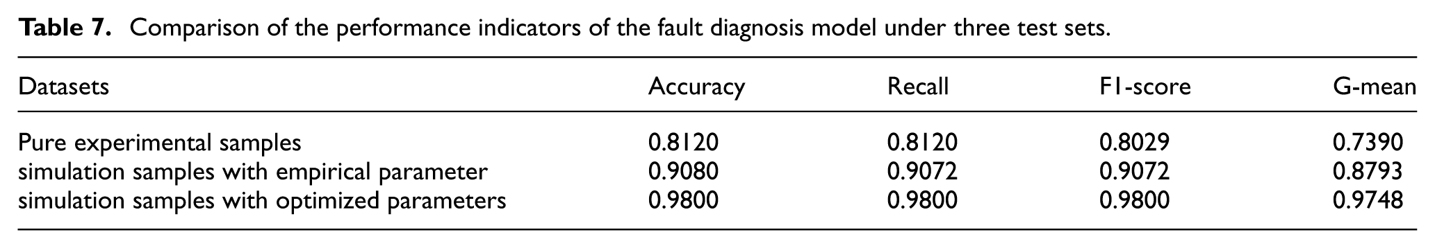
After training the diagnostic network with three training datasets, the diagnostic performance was evaluated using the test dataset. Four metrics, namely accuracy, recall, F1-score, and G-mean, were employed for the evaluation, as shown in Table 7. An analysis of the results of the three test sets from the perspectives of sample balance and optimization reveals that the pure experimental samples led to poor performance of the model in all metrics and an imbalance in the recognition of positive and negative samples due to insufficient data volume and uneven class distribution. The simulation samples with empirical parameters improved the sample distribution to some extent by increasing sample diversity, thereby enhancing the diagnostic performance, but still had limitations. In contrast, the simulation samples with optimized parameters significantly improved the sample quality and feature representation through precise parameter adjustment. They not only achieved a balanced distribution of sample classes but also provided the model with more abundant and accurate feature information. In key metrics such as accuracy (0.98), recall (0.98), F1-score (0.98), and G-mean (0.9748), these samples far outperformed the other test sets, effectively enhancing the model’s ability to diagnose various faults in axial piston pumps. This validates the significant value of sample optimization and balancing strategies in improving the performance of fault diagnosis models.

Table 7.

Comparison of the performance indicators of the fault diagnosis model under three test sets.

Datasets	Accuracy	Recall	F1-score	G-mean
Pure experimental samples	0.8120	0.8120	0.8029	0.7390
simulation samples with empirical parameter	0.9080	0.9072	0.9072	0.8793
simulation samples with optimized parameters	0.9800	0.9800	0.9800	0.9748

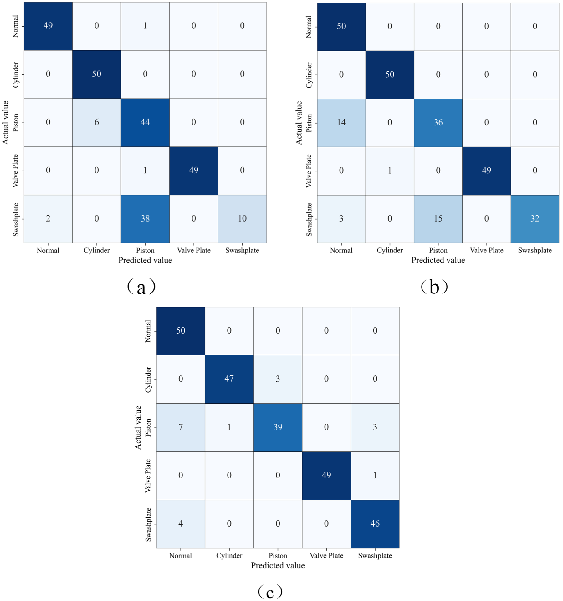
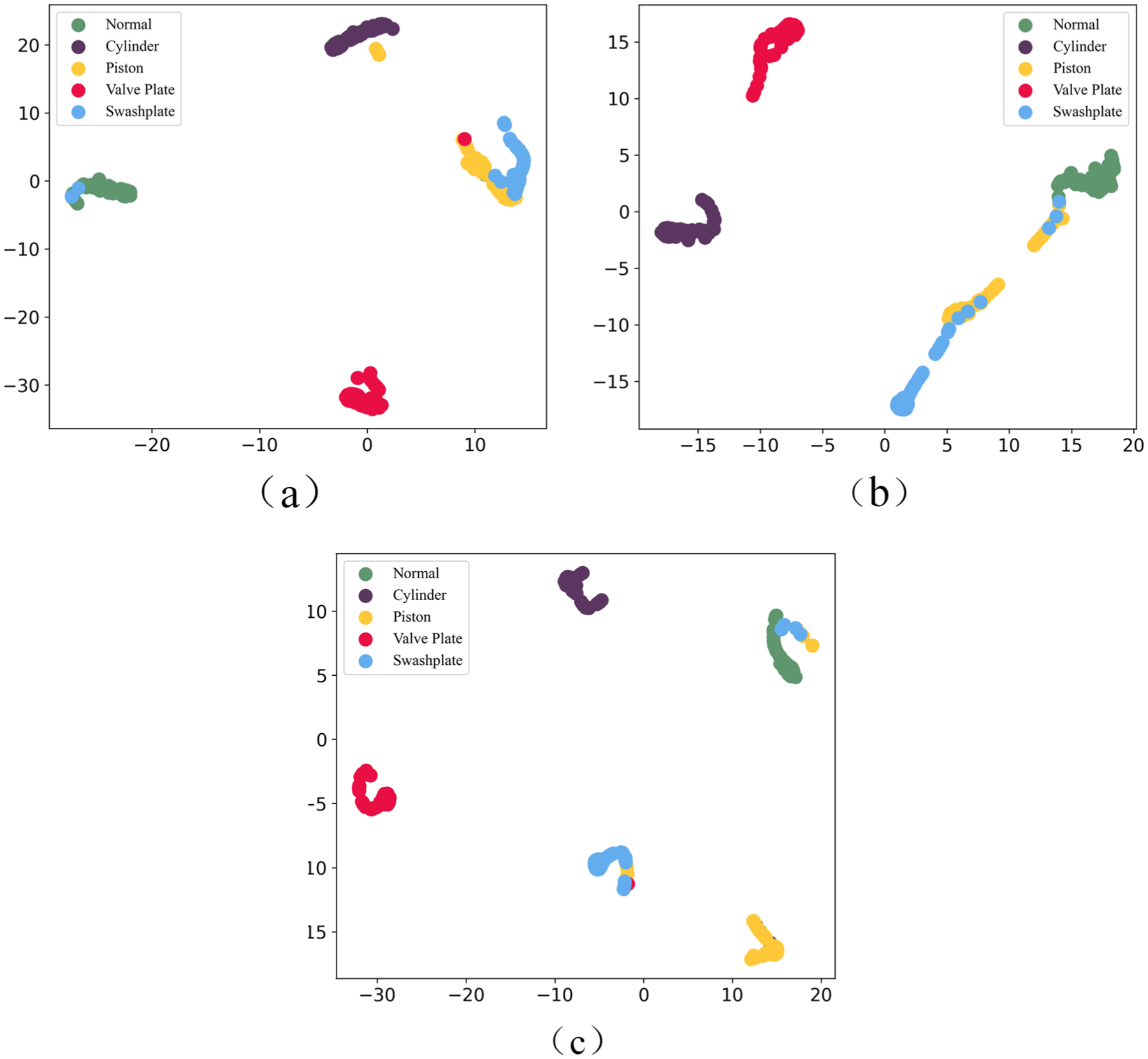
As shown in Figure 13 (confusion matrix) and Figure 14 (t-SNE), the three test sets differ significantly in validating the axial piston pump fault diagnosis model, revealing how sample optimization impacts model performance. Pure experimental samples, limited by small data size and imbalanced classes, show numerous misjudgments in the confusion matrix, especially for similar faults. The t-SNE plot shows randomly scattered data points with overlapping features, indicating poor feature extraction. Simulation samples with empirical parameters improve some diagnostic accuracies by diversifying samples but still have misclassifications. The t-SNE plot shows better clustering, yet highly related faults still overlap, reflecting limited feature discrimination. Optimized-parameter simulation samples stand out with high identification accuracy and negligible misjudgments in the confusion matrix. In the t-SNE plot, fault categories form distinct clusters with wide separations, proving that parameter optimization and sample balancing enhance the model’s ability to distinguish complex faults, offering an effective approach to boost diagnostic performance.

Figure 13.

Confusion matrix diagram of axial piston pump fault data under different test sets (Case I: few samples).

Figure 14.

t-SNE dimensionality reduction clustering diagram of axial piston pump fault data under different test sets (Case I: few samples).

Case II: Missing data for a working condition

To further evaluate the proposed framework, Case II considers a more extreme and practical situation: the experimental data for a specific fault under a given working condition are entirely missing, presenting a more rigorous test of the diagnostic methodology.

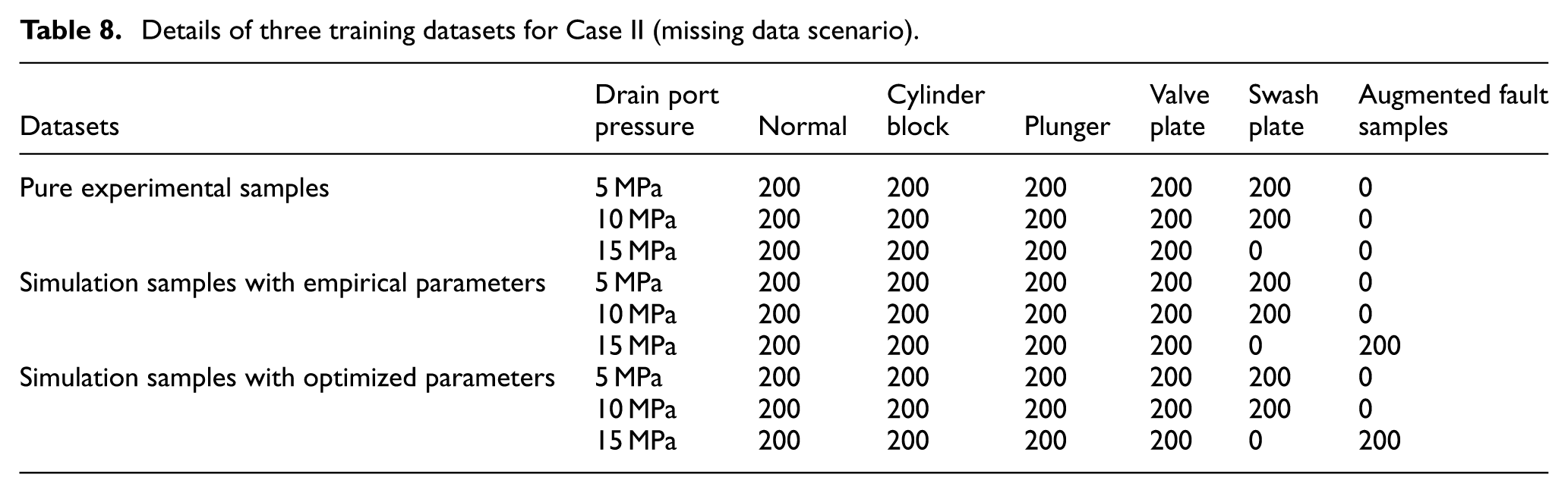
Under three discharge pressure conditions of 5, 10, and 15 MPa, the normal state, cylinder block fault, plunger fault, and valve plate fault each have 650 samples. However, for the swash plate fault under the 15 MPa condition, samples are severely lacking, resulting in a notably imbalanced sample distribution. To compensate for this, 200 swash plate fault samples were generated directly using simulation data based on IPINN-optimized parameters to supplement this category. For comparison, an equal number of simulation samples were generated simultaneously using empirical parameters. Consequently, three types of training sets were constructed: the pure experimental dataset, the empirical-parameter simulation dataset, and the optimized-parameter simulation dataset, with their specific compositions detailed in Table 8. During the testing phase, 50 samples were selected from each state to form the test set. Fault diagnosis was performed using the BiTCN model, with its training parameters consistent with those in Case 4.1.

Table 8.

Details of three training datasets for Case II (missing data scenario).

Datasets	Drain port pressure	Normal	Cylinder block	Plunger	Valve plate	Swash plate	Augmented fault samples
Pure experimental samples	5 MPa	200	200	200	200	200	0
	10 MPa	200	200	200	200	200	0
	15 MPa	200	200	200	200	0	0
Simulation samples with empirical parameters	5 MPa	200	200	200	200	200	0
	10 MPa	200	200	200	200	200	0
	15 MPa	200	200	200	200	0	200
Simulation samples with optimized parameters	5 MPa	200	200	200	200	200	0
	10 MPa	200	200	200	200	200	0
	15 MPa	200	200	200	200	0	200

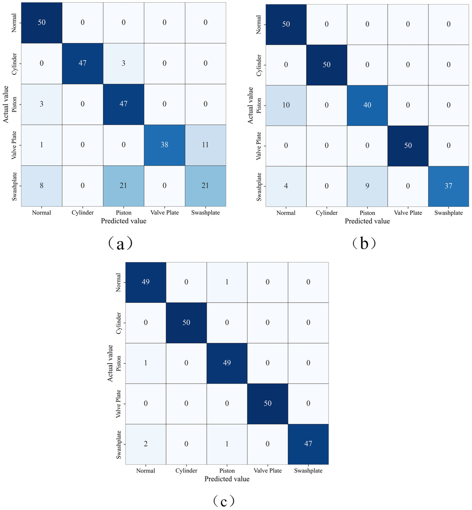
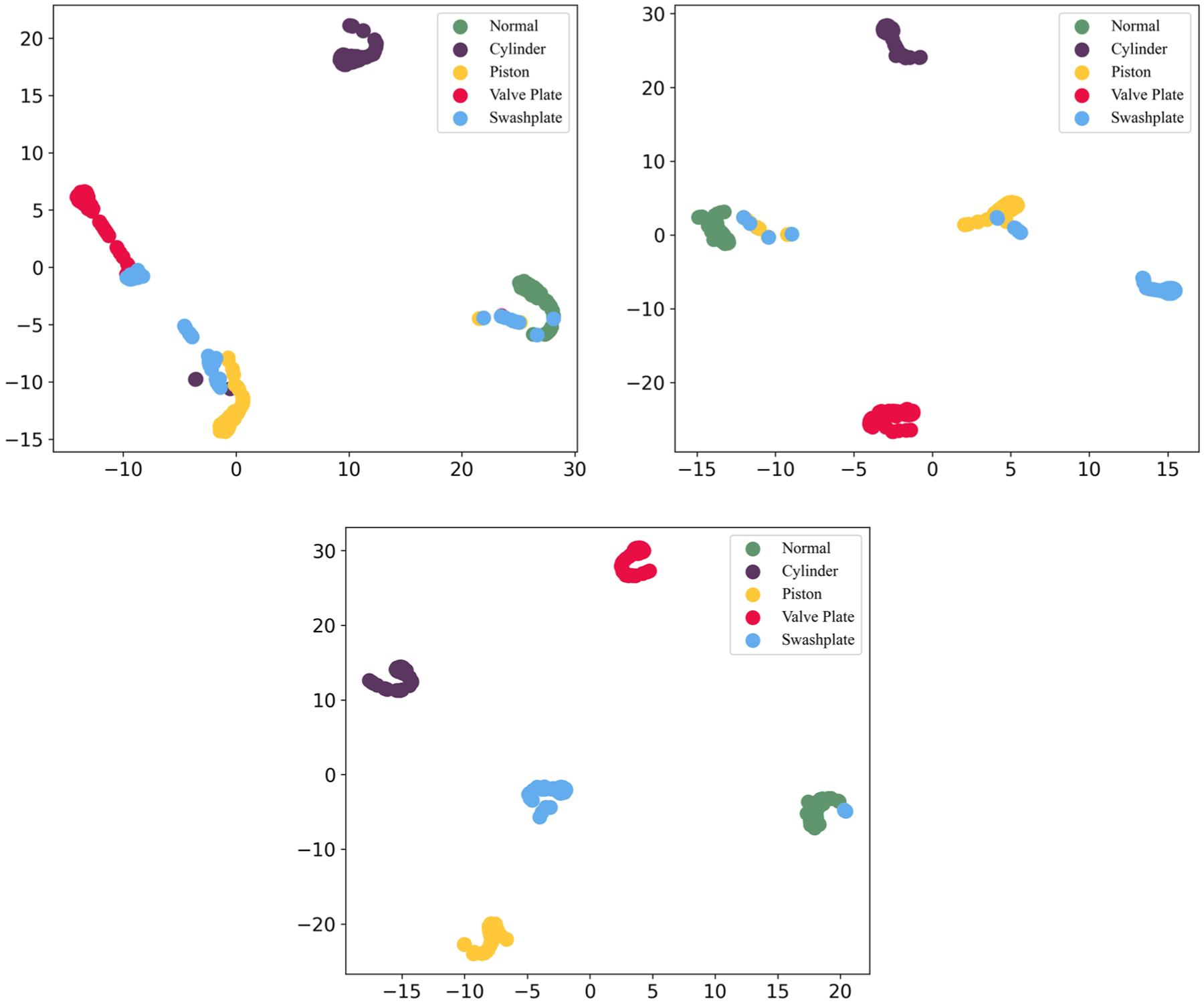
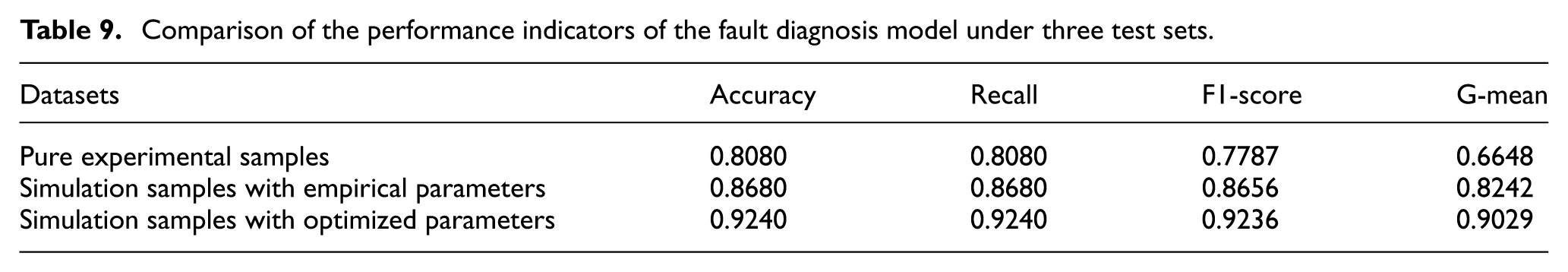
The diagnostic results indicate that the model trained with pure experimental samples showed poor performance in diagnostic indicators due to data absence, making it difficult to accurately identify faults. Although the simulation sample set with empirical parameters increased the sample size, the improvement in diagnostic performance was limited. By contrast, the simulation sample set with optimized parameters significantly improved sample quality, enabling the model to achieve excellent performance in metrics such as accuracy, recall, F1-score, and G-mean, reaching 0.9240, 0.9240, 0.9236, and 0.9029 respectively, far surpassing the other two groups. Detailed comparisons of performance metrics are listed in Table 9. As shown in Confusion Matrix Figure 15 and t-SNE Visualization Figure 16, the simulation sample set with optimized parameters had extremely few misjudgments and clear data clustering, fully verifying the effectiveness and superiority of the proposed method in addressing data absence issues and demonstrating its capability to significantly enhance the performance of fault diagnosis models.

Table 9.

Comparison of the performance indicators of the fault diagnosis model under three test sets.

Datasets	Accuracy	Recall	F1-score	G-mean
Pure experimental samples	0.8080	0.8080	0.7787	0.6648
Simulation samples with empirical parameters	0.8680	0.8680	0.8656	0.8242
Simulation samples with optimized parameters	0.9240	0.9240	0.9236	0.9029

Figure 15.

Confusion matrix diagram of axial piston pump fault data under different test sets (Case II: missing data).

Figure 16.

t-SNE dimensionality reduction clustering diagram of axial piston pump fault data under different test sets (Case II: missing data).

Compare with different algorithms

In the field of axial piston pump fault diagnosis, the reliability and stability of algorithm performance are of crucial importance. To further verify the advantages of the method proposed in this paper, which is based on IPINN and BiTCN, 10 repeated experiments were conducted using the “simulation samples with optimized parameters” training set in Section 4.1. This method was compared and analyzed with classic neural network algorithms such as TCN, LSTM, BiLSTM, and BiGRU. The experiments strictly adhered to the sample selection and model training parameter settings in Section 4.1.

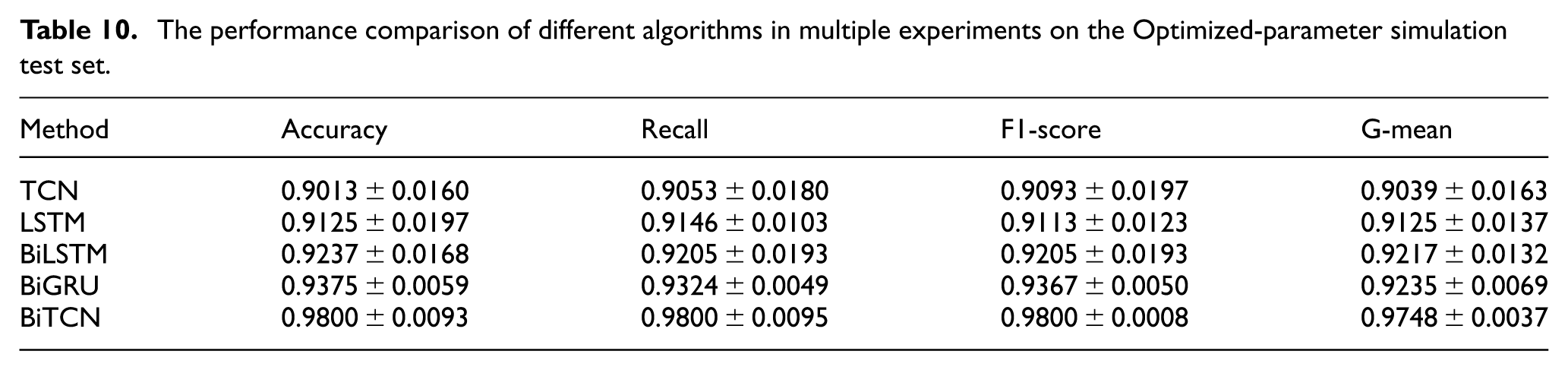
After completing the 10 experiments, the accuracy, recall rate, F1-score, and G-mean of each model were recorded, and the results are presented in Table 10. BiTCN performed best, with the average values of its indicators reaching 0.9800, 0.9800, 0.9800, and 0.9748 respectively, far surpassing those of other algorithms. The average values of the indicators for TCN, LSTM, BiLSTM, and BiGRU were all lower than those of BiTCN. It can be seen more intuitively from Figure 17 that BiTCN has a distinct advantage in all indicators. The dilated causal convolution, bidirectional structure, and SE attention mechanism of BiTCN enable it to handle time-series data in fault diagnosis more effectively.

Table 10.

The performance comparison of different algorithms in multiple experiments on the Optimized-parameter simulation test set.

Method	Accuracy	Recall	F1-score	G-mean
TCN	0.9013 ± 0.0160	0.9053 ± 0.0180	0.9093 ± 0.0197	0.9039 ± 0.0163
LSTM	0.9125 ± 0.0197	0.9146 ± 0.0103	0.9113 ± 0.0123	0.9125 ± 0.0137
BiLSTM	0.9237 ± 0.0168	0.9205 ± 0.0193	0.9205 ± 0.0193	0.9217 ± 0.0132
BiGRU	0.9375 ± 0.0059	0.9324 ± 0.0049	0.9367 ± 0.0050	0.9235 ± 0.0069
BiTCN	0.9800 ± 0.0093	0.9800 ± 0.0095	0.9800 ± 0.0008	0.9748 ± 0.0037

Figure 17.

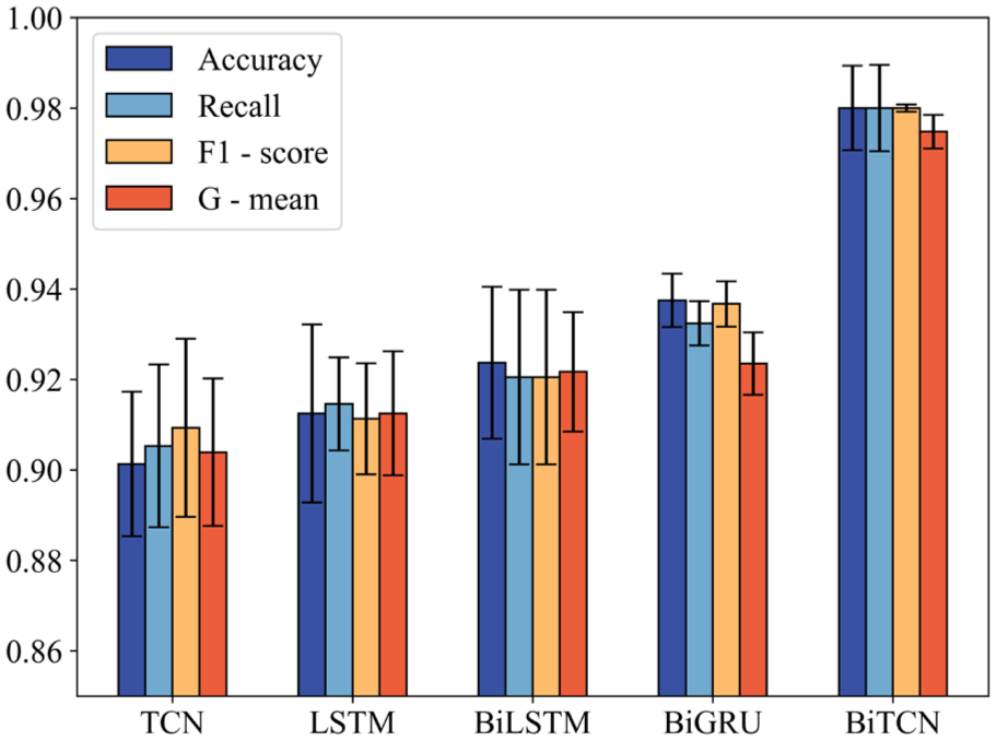
Comparison of performance indicators of different algorithms.

In conclusion, the experiments demonstrate that BiTCN has higher accuracy and stability in axial piston pump fault diagnosis, providing a better solution for fault diagnosis.

Ablation study

To evaluate the individual contributions of each component in the proposed BiTCN model, an ablation study was conducted. By removing specific modules one by one, their impacts on the fault diagnosis performance of axial piston pumps were analyzed to determine the importance of each module in the overall architecture and quantify the relative contributions of the dilated causal convolution, SE attention mechanism, and bidirectional residual structure. The baseline model was the complete BiTCN network model. Three network structures were considered in the experiment: Model A (replacing the dilated causal convolution with ordinary convolution), Model B (removing the SE attention mechanism), and Model C (removing the backward residual structure while retaining only the forward residual structure).

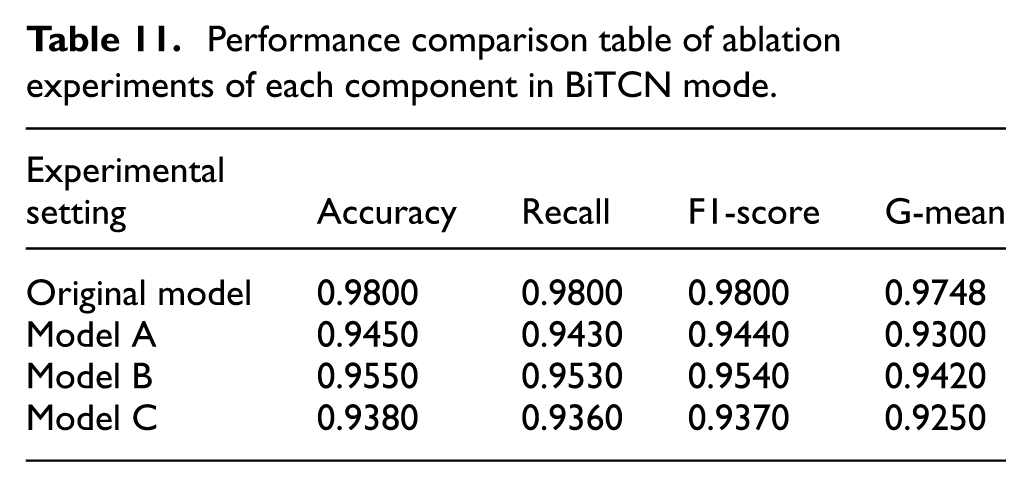
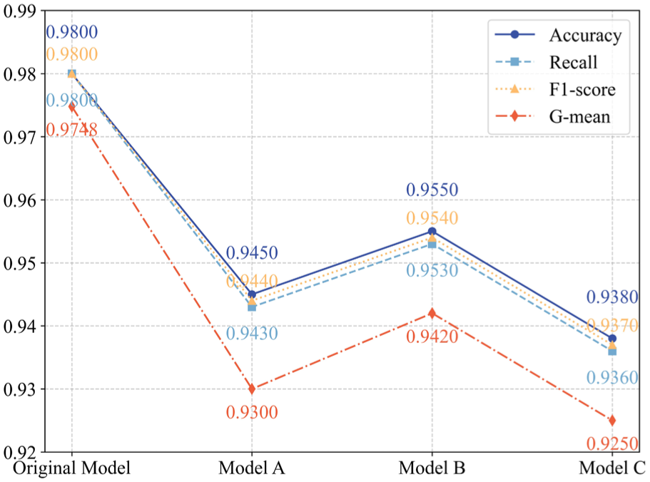
As shown in Table 11 and Figure 18, each component has a significant impact on performance. The significant decline in multiple performance indicators of Model A highlights the critical role of dilated causal convolution in processing time-series data. The performance changes of Model B demonstrate the value of the SE attention mechanism in feature focusing, while the results of Model C verify the necessity of the bidirectional structure in utilizing forward and backward time-series information.

Table 11.

Performance comparison table of ablation experiments of each component in BiTCN mode.

Experimental setting	Accuracy	Recall	F1-score	G-mean
Original model	0.9800	0.9800	0.9800	0.9748
Model A	0.9450	0.9430	0.9440	0.9300
Model B	0.9550	0.9530	0.9540	0.9420
Model C	0.9380	0.9360	0.9370	0.9250

Figure 18.

The performance comparison diagram of each component ablation experiment in BiTCN mode.

Compared with the complete BiTCN model, the accuracy rates of these models were lower, which verifies the necessity of each component. The complete BiTCN model also converged faster, further demonstrating its superiority.

Noise robustness analysis of the BiTCN model

Vibration signals collected in real industrial environments are often contaminated by varying degrees of background noise, posing a significant challenge to the stability and reliability of fault diagnosis models. To comprehensively evaluate the applicability of the proposed BiTCN diagnostic model in practical industrial settings, we systematically investigated the impact of different noise intensities on its diagnostic performance.

To simulate the noise interference encountered in real industrial environments, Gaussian white noise with different signal-to-noise ratios (SNR) was added to the test set constructed in Section 4.1. The signal-to-noise ratio is defined as:

$${\mathrm{SNR}}_{\mathrm{dB}}=10\mathrm{lo}{g}_{10}\left(\frac{P_{\mathrm{signal}}}{P_{\mathrm{noise}}}\right)$$

(24)

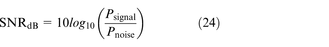
where P _signal and P _noise represent the power of the signal and the noise, respectively. In the experiment, five different SNR levels were set: ∞ (no noise), 20, 15, 10, and 5 dB. This range covers scenarios from ideal laboratory conditions to extremely harsh industrial environments. At each SNR level, the diagnostic performance of the BiTCN model was evaluated using the same test set, and compared with TCN, LSTM, and BiLSTM models. All models utilized parameters trained on clean data to ensure a fair comparison of their generalization capabilities and noise robustness.

The performance comparison of different diagnostic models under varying SNRs is illustrated in Figure 19. The experimental results clearly demonstrate that BiTCN maintains optimal performance across all noise environments. Under no-noise conditions, BiTCN achieves an accuracy of 0.980, significantly outperforming the other models. As the noise level increases, the performance of all models declines, but BiTCN exhibits the best robustness, with its accuracy curve declining the most gradually. Notably, even under strong noise conditions of 5 dB, BiTCN maintains an accuracy of 0.910, which is 9% and 11% higher than TCN and LSTM, respectively. This result fully demonstrates the stability and reliability of BiTCN under noise interference, highlighting its significant advantage for industrial field applications. The superior noise robustness can be attributed to BiTCN’s bidirectional temporal convolution structure, which effectively captures contextual information from both forward and backward time sequences, and its SE attention mechanism, which enhances focus on critical fault features while suppressing noise-induced disturbances.

Figure 19.

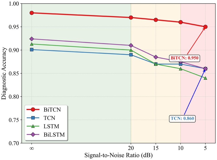
Performance comparison of different diagnostic models under varying signal-to-noise ratios.

Conclusion

This study proposes a novel fault diagnosis framework combining Inverse Physics-Informed Neural Networks (IPINN) and Bidirectional Temporal Convolutional Networks (BiTCN) for axial piston pumps under imbalanced samples. Through systematic methodological design and experimental validation, the following key conclusions are drawn:

• (1) The proposed IPINN method successfully mitigates sample imbalance by achieving accurate inversion of key dynamic parameters and generating high-fidelity simulation data. By integrating physical models with measured signals, it identifies a physically consistent parameter set, breaking the reliance on empirical estimations. The optimized data shows superior fidelity in both time and frequency domains. Augmenting scarce datasets with IPINN-generated data drastically improves diagnostic performance, raising accuracy from 0.812 to 0.98, and maintaining 0.9240 even under complete data absence. Visualization confirms clearer fault cluster separation, effectively alleviating overfitting caused by data imbalance.

• (2) The BiTCN model demonstrates exceptional diagnostic performance and strong noise robustness, outperforming traditional sequential models. In repeated experiments, it achieves the highest average accuracy, recall, F1-score (all 0.9800) and G-mean (0.9748) with superior stability. Ablation studies validate the critical roles of its dilated convolution, SE attention, and bidirectional structure. Under strong noise, BiTCN maintains 0.910 accuracy, outperforming TCN and LSTM by 9–11 percentage points, highlighting its practical value in noisy industrial environments. This highlights its practical value for real-world applications where signal contamination is inevitable, attributed to its ability to robustly extract multi-scale temporal features and focus on fault-related frequency components via the SE mechanism.

In summary, the IPINN-BiTCN framework addresses the critical challenge of fault diagnosis under imbalanced samples through a two-pronged approach: IPINN provides physics-informed, high-quality data generation and balancing, while BiTCN delivers a high-performance, robust classifier. This integrated methodology offers an effective and innovative solution for accurate and reliable fault diagnosis of axial piston pumps, establishing a solid foundation for subsequent research and intelligent maintenance strategies. The optimization results for the swash plate fault scenario demonstrate the output of this general IPINN framework for a specific case. Systematically extending this framework to other fault types (e.g. piston, cylinder block, and valve plate faults) and uncovering the mapping between parameter optimization patterns and underlying fault physics constitute the core future research direction envisioned in this work.