Sage Journals: Discover world-class research

Abstract

Unsteady aerodynamics can significantly affect the design of highly maneuverable aircraft that fly at high angles of attack. Conventional modeling methods, such as polynomial methods or lookup tables, are of limited value. This investigation was motivated by the need for an accurate and simplified prediction of unsteady aerodynamics by modeling experimental data. Such modeling is important for preliminary aircraft design purposes and control law development, which is a challenging problem when considering a highly nonlinear aerodynamic loading model. In this study, a neuro-fuzzy (NF) model developed using experimental data was favorably compared with other modeling techniques and semi-empirical methods. The model uses three inputs (angle of attack, non-dimensional pitch rate, and aspect ratio) and outputs the aerodynamic normal force coefficient, which was found with a root mean square error of less than 6% for an angle of attack range of 0°–90°. The proposed NF modeling procedure is demonstrated and recommended for use with other aerodynamic force coefficients as the new model outputs. The minimum and maximum angles of attack should be used as model inputs to improve model accuracy for multiple ranges of angles of attack.

Keywords

AI neuro-fuzzy angle of attack

Introduction

In aerodynamics, laminar airflow is smooth and orderly, reducing drag and improving fuel efficiency and performance, while turbulent airflow is chaotic, increasing drag and energy loss. Laminar flow creates less disruptive wake turbulence, enhancing safety for trailing aircraft, whereas turbulent airflow (vortex) may produce significant wake vortices that pose hazards, especially to smaller aircraft following larger ones.¹ Furthermore, to reduce the airplane, drag force, designers optimize the aircraft’s shape for smooth airflow, ensuring surfaces are clean and free of debris. Many aerodynamic designs can be applied for that purpose such as winglets and streamlined fuselage contours to reduce parasitic drag. Modern aircraft are designed to operate under unsteady aerodynamics and at high angles of attack. For example, tactical fighters and other aircraft types can reach 90° and execute controlled transient maneuvers beyond the stall angle. This capability requires fly-by-wire control, thrust vectoring, and low-aspect-ratio (AR) lifting surfaces for airflow control at high angles of attack. Delta wings and their flight envelopes, which include extremely high angles of attack, were critical in this case. These requirements have motivated several experimental attempts to investigate and model complex unsteady aerodynamics, including the characteristics of flow separation, vortex sheets, and vortex bursting. In existing flight simulations, few methods are commonly used to address unsteady aerodynamics attributed to high angles of attack.^2–7 Although some conventional approaches to system modeling perform poorly in handling complex nonlinear systems, where it is difficult to find a global functional or analytical structure, artificial intelligence (AI), particularly neuro-fuzzy (NF) logic, can help model such complex systems. Fuzzy logic (FL) is developed as a mathematical framework to solve uncertainty. In traditional logic, true and false statements are used, while (FL) allows for degrees of truth between 0 and 1.⁸ FL is suitable for handling problems in real-world scenarios that involve vagueness and ambiguity. Aslan et al.⁹ utilized FL for Model reference adaptive controllers (MRACs), which are widely employed in various industrial application areas due to their adaptability to variable conditions. FL was proposed to improve MRAC performance. This methodology is employed in the current study. On the other hand, Machine Learning (ML) is a computational algorithm developed to perform a task without being explicitly programed. This enables computers to learn and make predictions or decisions based on data. ML has various types of algorithms mainly; supervised learning, unsupervised learning, and reinforcement learning.^10,11 The author in Ref.¹² conducted a study to check the appropriateness of Fuzzy Logic (FL) to model unsteady aerodynamics where it was found promising and hence carried out the full investigation as presented in this paper and extensively discussed in the next sections.

Talpur et al.¹³ conducted a thorough investigation and indicated that in recent years, deep neural networks (DNN) have made significant strides in handling large and complex datasets, albeit criticized for their black-box nature. This criticism has spurred the exploration of hybrid approaches, leading to the development of novel systems termed deep neuro-fuzzy systems (DNFS). Research on DNFS implementation has surged across various domains like computing, healthcare, transportation, finance, and aerospace offering high interpretability and reasonable accuracy. Talpur et al. study undertakes a systematic review to assess the current progress, trends, challenges, and future scope of DNFS research. The study identifies and analyzes 105 relevant publications between 2015 and 2020. Findings indicate active growth in DNFS research with significant potential for future applications. Tumse et al.¹⁴ conducted a study aimed to create a monthly average Heat Index (HI) map for Türkiye using a mathematical model by AccuWeather, an artificial neural network (ANN), and an adaptive neuro-fuzzy inference system (ANFIS). Using data from 81 measuring stations, including temperature, humidity, wind speed, and atmospheric pressure; it was found that HI can be efficiently predicted in locations lacking data through ANN and ANFIS methods. The models demonstrated good agreement with actual HI values, though ANN outperformed ANFIS in accuracy. Both models effectively predict HI using geographical inputs, reducing the need for extensive testing and saving resources.

Fuzzy logic (FL) techniques have been successfully utilized to model nonlinear unsteady aerodynamics. The angle of attack (α), side-slip angle, and elevator deflection were used as FL inputs to reasonably predict the aerodynamic coefficients.¹⁵ Furthermore, FL was investigated using aerodynamic data obtained from forced pitching and rolling oscillations at high angles of attack, which shows that it can effectively predict unsteady aerodynamics.¹⁶ Other AI techniques, such as recurrent neural networks, have been used to identify aerodynamic stalls at high angles of attack. For instance, Zhang et al.¹⁷ used recurrent neural networks with training data obtained from a computational fluid dynamics method to investigate the unsteady aerodynamic parameters of an NACA0012 airfoil. Machine learning techniques have been widely applied across diverse fields, including complex engineering applications. Li et al.¹⁸ leveraged machine learning to model the intricate structures of aeroengine turbine rotors. Their study focused on evaluating the reliability performance of turbine rotors, characterized by multiple correlated failure modes. To address this challenge, they proposed a Vectorial Surrogate Model (VSM) method, which integrates a linkage sampling technique and a model updating strategy. This innovative approach was tested on a typical high-pressure turbine rotor, considering correlated failure modes such as deformation, stress, and strain failures. The proposed method enabled the researchers to obtain critical insights, including response distributions, reliability degrees, sensitivity metrics, and correlation relationships between the failure modes. Comparative analyses demonstrated that the VSM method outperformed existing approaches by providing an efficient and accurate probabilistic evaluation of multi-failure correlations.

Pradhan et al.¹⁹ employed a Convolutional Neural Network (CNN) combined with Shapley Additive Explanation (SHAP) for geological mapping and the exploration of gold mineral prospects. Their study aimed to model known gold occurrences about multiple thematic layers, facilitating the replication of results in adjacent regions. The findings revealed that the central parts of the study area exhibited a significantly higher gold prospect potential compared to surrounding regions. A cascade ensemble learning (CEL) approach was developed using a wavelet neural network-based AdaBoost model and a cascade synchronous strategy (CSS) for multi-level reliability analysis. This innovative approach offers a heuristic framework for evaluating the multi-level reliability of complex aerospace engineering systems. Applied to a turbine rotor system, the method provided insights into reliability performance under varying operating conditions and multiple failure modes. Specifically, it quantified the failure correlations across three operating conditions (90%, 95%, and 100% loading) and three failure modes: deformation, stress, and strain. The results validated the effectiveness of the proposed method in modeling and simulating complex engineering systems from a system-engineering perspective. Despite its strengths, the method has limitations. The current validation case considers only maximum deformation, stress, and strain as failure modes. Additional research is needed to extend its applicability to more complex failure scenarios, such as low-cycle and high-cycle fatigue. Given the pervasive challenges of reliability evaluation and optimization in aerospace systems, the approach holds promising potential for broader applications in various engineering fields requiring robust analysis under complex operating conditions and multiple failure modes.²⁰

Machine learning techniques can be suitable and reliable, depending on the system being investigated.²¹ Given the importance of supermaneuvrability in the design of advanced aircraft, unsteady aerodynamics has been a popular topic in both experimental and theoretical investigations. For example, Jarrah²² conducted an experimental program on unsteady aerodynamics to measure the aerodynamic forces of maneuvering delta wings with ARs of 1, 1.5, and 2. The data obtained by Jarrah²² were used in the current study for NF modeling, which represents the aerodynamics of advanced fighter super maneuvers at high angles of attack up to 90°. Bragg et al.²³ studied the aerodynamic loads on a delta wing oscillating up to a post-stall angle of attack. The aerodynamic load coefficients (lift, drag, normal force, rolling moment, and pitching moment) were obtained and plotted for various Reynolds numbers and reduced frequencies at the side-slip angles of 0°, 5°, and 15°. An appreciable aerodynamic load hysteresis was observed, and the effect of the Reynolds number was moderate. Several other relevant investigations have been conducted to date. Ericsson²⁴ presented an analysis based on small perturbations in the mean static α. Superposition was used to obtain unsteady aerodynamic derivatives, and Smith²⁵ reviewed theoretical methods for predicting steady and unsteady separated flows over wings at high angles of attack. Tumse et al.²⁶ investigated machine learning techniques to estimate the aerodynamic coefficients of a 40° swept delta wing under ground effect using three approaches: feed-forward neural network (FNN), Elman neural network (ENN), and adaptive neuro-fuzzy inference system (ANFIS). The optimal configurations of these models were compared, with ENN emerging as the most accurate. The models predicted the lift (CL) and drag (CD) coefficients at a ground proximity of h/c = 0.4 using data from h/c = 1, 0.7, 0.55, 0.25, and 0.1 (h/c refers to the ratio of the height h above the ground to the chord length c of the wing. Inputs included the angle of attack (α) and ground distance (h/c), with outputs being C_L and C_D. The ENN achieved the highest accuracy, with 1.0709% MAPE, 0.00595 RMSE, and 0.00504 MAE for C_L prediction, outperforming FNN and ANFIS. Results demonstrate that these models can effectively forecast the aerodynamic coefficients underground effect, reducing the need for extensive experimental measurements and associated costs. Zhang et al²⁷ used a promising data-driven approach to predict the thrust of the rocket engine by employing a deep neural network architecture. They extracted advanced features from the preprocessed data to predict solid rocket motor thrust.

Tümse et al.²⁸ studied wind energy due to the significant attention it received over the last decade, with wind speed being the most critical factor influencing the power output from wind turbines. Due to the unstable nature of wind, it is challenging to establish a direct theoretical relationship between wind power and speed, making simulation essential. Their study predicted wind turbine power (P) using three forecasting methods: adaptive neuro-fuzzy inference system (ANFIS), Elman neural network (ENN), and feed-forward neural network (FNN). The models were trained using wind speed (V) and turbine rotor speed (ṅ) from a dataset of 43,800 entries, with 80% for training and 20% for testing. ANFIS outperformed ENN and FNN, showing lower mean absolute error (MAE) and root mean square error (RMSE) in both stages. Specifically, ANFIS achieved 52.448 kW MAE and 87.204 kW RMSE during training, and 48.675 kW MAE and 78.453 kW RMSE during testing. The coefficient of determination (R²) for ANFIS was 0.9948 in training and 0.9961 in testing, slightly higher than ENN and FNN. Thus, ANFIS proves effective for estimating wind power, reducing the need for extensive experimental measurements and associated costs.

Jarrah²² and Bragg et al.²³ were most relevant to this investigation, and their experimental data were compared with the NF model outputs. Classical logic cannot simulate the human brain’s approach to abstract decision making. Human expertise is provided by fuzzy linguistic expressions (e.g. when the flow is unsteady), which can be considerably useful if modeled. The FL developed by Zadeh²⁹ is a form of many-valued logic used to model complex systems influenced by human decisions based on imprecise and non-numerical information. To date, FL has been used in many applications, including control systems, decision-making processes, language processing, automotive systems, and aerospace applications.³⁰ FL modeling involves appropriately selecting the universe of information and partitioning it into several fuzzy sets represented by membership functions (MFs) that uniformly cover the universe range. MFs are mathematical expressions with subjective parameters that depend on the individual differences in the perception and expression of abstract concepts. Furthermore, MFs are represented by a curve that relates each point in the input space to a membership value between zero and one, known as the degree of membership. The most commonly used MFs investigated and implemented in this study are shown in Figure 1.

Figure 1.

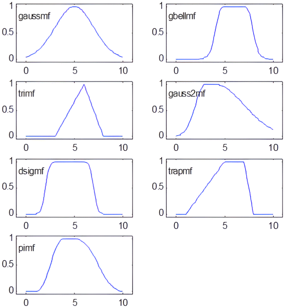
Various types of the most commonly used membership functions.

To date, many investigations have been conducted to determine the MFs that yield the best FL performance. For example, Simon³¹ proposed an optimization approach that ensured that the resulting MFs were normal, which is desirable for its natural appeal and easier real-time implementation of FL systems. Many other strategies to select the MFs that are most appropriate for providing an optimal-performance FL model have been investigated and discussed.³² For example, Sugeno and Tanaka³³ suggested a method for successive identification of a fuzzy model. This method involves two levels. The first level (supervisor) determines the parameter adjustment policy using a set of fuzzy adjustment rules derived from the fuzzy implications of a fuzzy model. The second level (adjustment level) executes the parameter adjustment policy determined by the fuzzy adjustment rules. Two major fuzzy inference systems differ in the manner in which their rules are aggregated and defuzzified: Mamdani, which was initially used to control a steam engine with linguistic rules, and Sugeno, developed by Takagi, Sugeno, and Kang.³⁴ The main difference between these two systems is that the rule conclusion of the former is a fuzzy set, whereas that of the latter is a crisp value or a function. The preference between the Mamdani and Sugeno types is problem-dependent; the Sugeno method is preferred if numerical data are available.³⁵ The manner in which fuzzy rules are produced facilitates the incorporation of the human knowledge of a target system into the fuzzy model. The Sugeno system is also referred to as an adaptive-network-based fuzzy inference system,³⁶ wherein the rule conclusion is a crisp value or function. A fuzzy system with two inputs (x, y) and two rules (Figure 2) has five layers, each having a number of nodes with similar functions.

Figure 2.

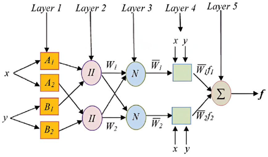
Equivalent adaptive network-based fuzzy inference system architecture for the two-input and two rules first-order Sugeno fuzzy model.

In the next sections various mathematical models were discussed and compared with the investigated modeling method. Followed by detailed analysis and discussion of results. The conclusion is presented highlighting the paper’s main outcomes and future works.

Mathematical model

In this study, NF modeling was performed using experimental data obtained from different resources. The characteristics of these experiments and the obtained data were analyzed to select the appropriate inputs and outputs for the NF models.

Jarrah’s experiment

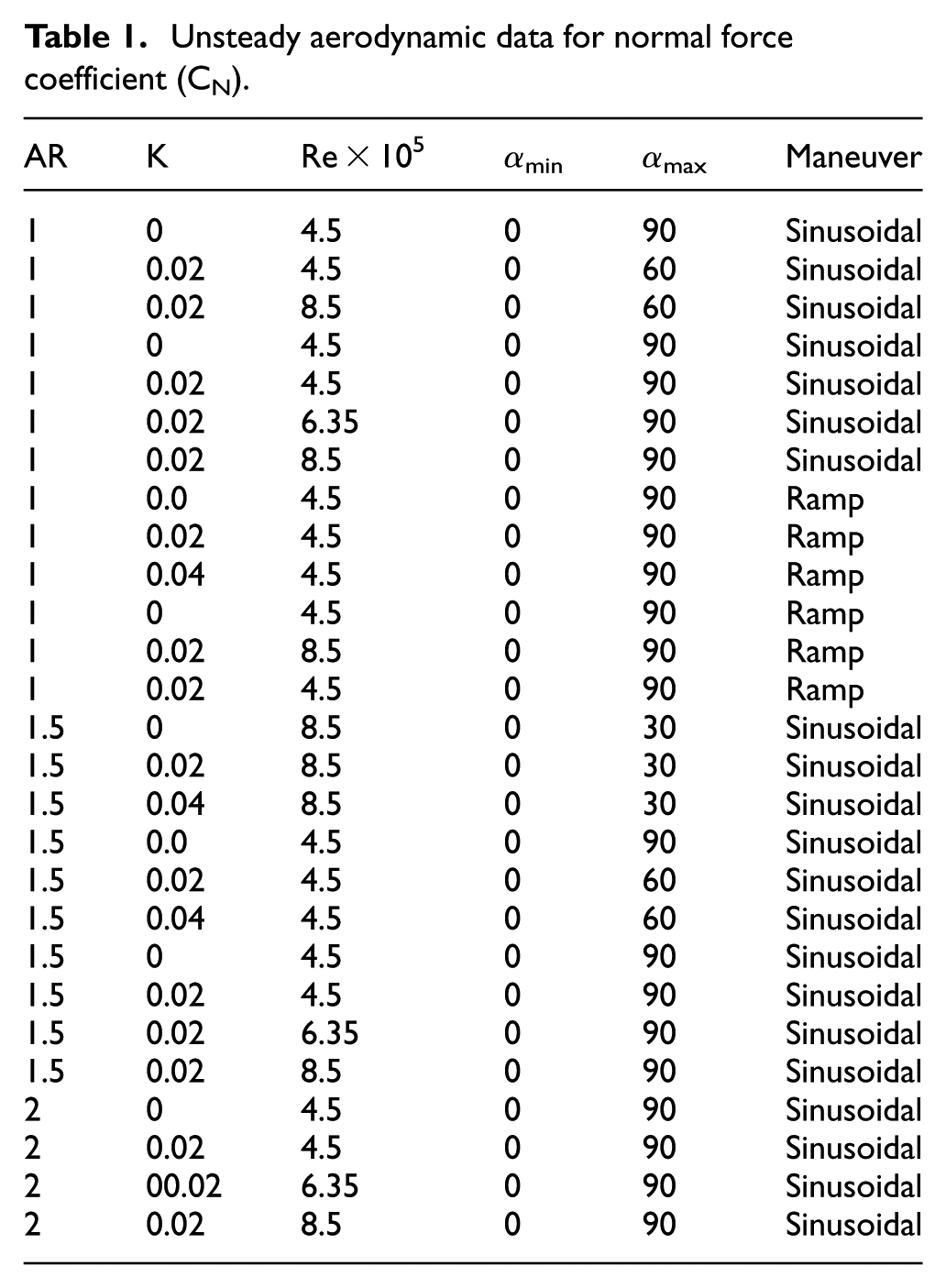
Jarrah’s experiment²² generated a large amount of data; however, only representative data for typical and important cases were selected and discussed in this study (Tables 1 and 2) to illustrate the effects and interactions of the following parameters: α, (AR), and rate of change of the angle of attack ( $\overset{\cdot}{α}$ ) through the presentation of the non-dimensional pitch rate (K), maximum and minimum angles of attack ( $α_{\max}$ and $α_{\min}$ ), and Reynolds number (Re). The rolling moment coefficient ( $C_{RM}$ ) was part of the experiment and was obtained for all modes. However, it had a very small effect compared to that of the other coefficients. Therefore, the following analysis considered only four aerodynamic coefficients: ( $C_{L}$ ), ( $C_{N}$ ), ( $C_{D}$ ), and ( $C_{M}$ ). However, in this study, only ( $C_{N}$ ) is used as the output of the NF model, and the other aerodynamic coefficients could be modeled similarly. The analysis is presented for AR = 1, 1.5, and 2, wherein the data are grouped into three α ranges: low-to-moderate (0°–30°), low-to-high (0°–60°), and low-to-extremely high (0°–90°). This order of analysis was performed for sinusoidal maneuvers, followed by ramp maneuvers, for each AR. The analysis was based on the data presented in Tables 1 and 2. The essential parameters affecting aerodynamic forces include α, AR, $\overset{\cdot}{α}$ , $α_{\max}$ , and $α_{\min}$ . Hence, $C_{N}$ can be written as:

C_{N} = f (α, \overset{\cdot}{α}, A R, α_{m i n}, α_{m a x}) .

(1)

Table 1.

Unsteady aerodynamic data for normal force coefficient (C_N).

AR	K	Re × 10⁵	α_max	Maneuver
1	0	4.5	90	Sinusoidal
1	0.02	4.5	60	Sinusoidal
1	0.02	8.5	60	Sinusoidal
1	0	4.5	90	Sinusoidal
1	0.02	4.5	90	Sinusoidal
1	0.02	6.35	90	Sinusoidal
1	0.02	8.5	90	Sinusoidal
1	0.0	4.5	90	Ramp
1	0.02	4.5	90	Ramp
1	0.04	4.5	90	Ramp
1	0	4.5	90	Ramp
1	0.02	8.5	90	Ramp
1	0.02	4.5	90	Ramp
1.5	0	8.5	30	Sinusoidal
1.5	0.02	8.5	30	Sinusoidal
1.5	0.04	8.5	30	Sinusoidal
1.5	0.0	4.5	90	Sinusoidal
1.5	0.02	4.5	60	Sinusoidal
1.5	0.04	4.5	60	Sinusoidal
1.5	0	4.5	90	Sinusoidal
1.5	0.02	4.5	90	Sinusoidal
1.5	0.02	6.35	90	Sinusoidal
1.5	0.02	8.5	90	Sinusoidal
2	0	4.5	90	Sinusoidal
2	0.02	4.5	90	Sinusoidal
2	00.02	6.35	90	Sinusoidal
2	0.02	8.5	90	Sinusoidal

Table 2.

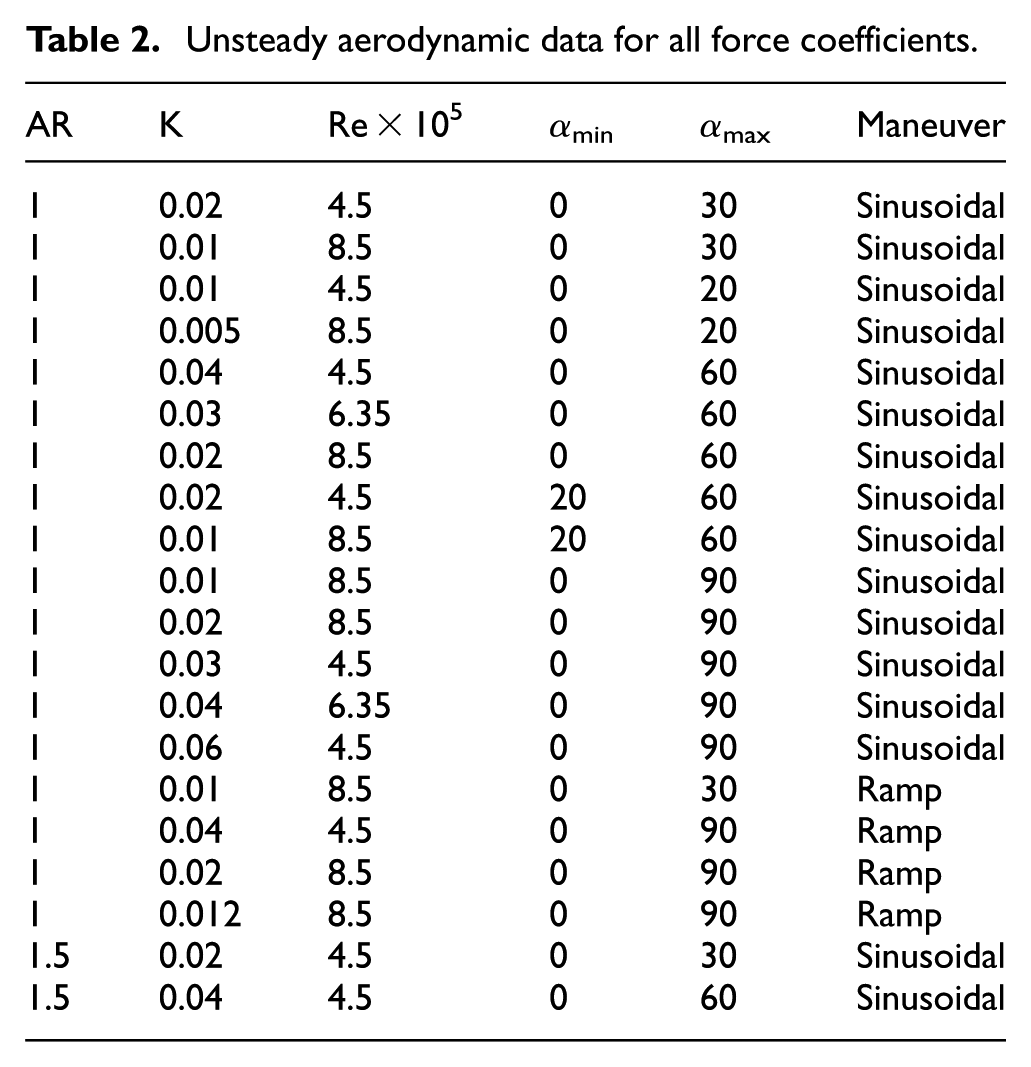
Unsteady aerodynamic data for all force coefficients.

AR	K	Re × 10⁵	α_min	α_max	Maneuver
1	0.02	4.5	0	30	Sinusoidal
1	0.01	8.5	0	30	Sinusoidal
1	0.01	4.5	0	20	Sinusoidal
1	0.005	8.5	0	20	Sinusoidal
1	0.04	4.5	0	60	Sinusoidal
1	0.03	6.35	0	60	Sinusoidal
1	0.02	8.5	0	60	Sinusoidal
1	0.02	4.5	20	60	Sinusoidal
1	0.01	8.5	20	60	Sinusoidal
1	0.01	8.5	0	90	Sinusoidal
1	0.02	8.5	0	90	Sinusoidal
1	0.03	4.5	0	90	Sinusoidal
1	0.04	6.35	0	90	Sinusoidal
1	0.06	4.5	0	90	Sinusoidal
1	0.01	8.5	0	30	Ramp
1	0.04	4.5	0	90	Ramp
1	0.02	8.5	0	90	Ramp
1	0.012	8.5	0	90	Ramp
1.5	0.02	4.5	0	30	Sinusoidal
1.5	0.04	4.5	0	60	Sinusoidal

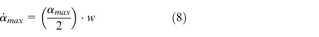
The effect of K is integrated in the model through $\overset{\cdot}{α}$ as

{\overset{\cdot}{α}}_{\max} = 2 (U_{\infty} . K) / C_{R} .

(2)

The time history of α used to obtain the experimental data is

α = (α_{\max} / 2) \cdot (1 - \cos (wt)) .

(3)

Therefore,

wt = co s^{- 1} (1 - \frac{2 α}{α_{\max}}) .

(4)

w (t) = si n^{- 1} (1 - \frac{2 \overset{\cdot}{α}}{α_{\max}}) .

(5)

\overset{\cdot}{α} = \pm 2 \cdot (U_{\infty} \cdot K) / [C_{R} \cdot \sin (w (t))]

(6)

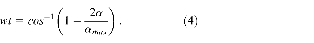
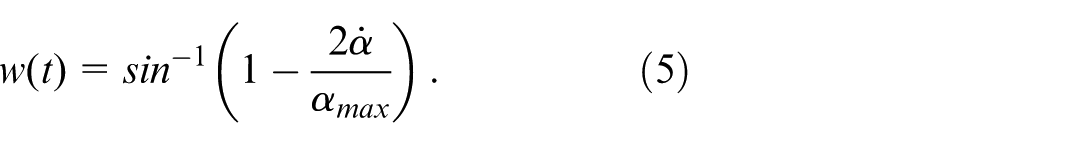
where the ± signs in equation (6) correspond to the pitch-up and pitch-down motions, respectively.

Bragg’s experiment

Bragg et al.²³ conducted an experiment on a simple flat-plate delta wing with a 70° leading-edge sweep using a 5 × 3 × 8 inch wind tunnel to investigate the aerodynamic forces and moments. The wing was made of 0.5-inch-thick plywood with a 20.61-inch root chord and sharp leading and trailing edges. They applied a sinusoidal pitching motion from 0° to 55°, with a steady side-slip angle of up to 15° in increments of 5°. The reduced frequency was kept constant by varying the oscillation frequency with the tunnel speed. A potentiometer was used to determine the instantaneous α. The wing was pitched at ∼57% of the root chord. The z-location of the pitch axis was at about 3.12 inch below the wing chord line. Velocity measurements were performed using a hot-wire probe and pressure transducer. Through data acquisition and reduction procedures, the dynamic data were digitally filtered using an average of several cycles at a sample rate based on the reduced frequency. The data recorded for each angle were the average of several hundred samples over a period of 10–15 s. The second input of the NF model is $\overset{\cdot}{α}$ , which is directly affected by the non-dimensional pitch rate coefficient (K) through equation (7). Therefore, the definition directly influences model prediction. Jarrah²² and Bragg et al.²³ used different definitions of K.

Jarrah defines K as

K = {\overset{\cdot}{α}}_{\max} (\frac{C}{2}) / U

(7)

{\overset{\cdot}{α}}_{\max} = (\frac{α_{\max}}{2}) \cdot w

(8)

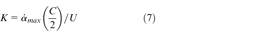
Bragg et al. define K as

K_{b} = w \cdot C / U

(9)

K = (α_{\max} / 4) \cdot k_{b}

(10)

According to equation (9), the following K_b values were expressed in terms of the Jarrah definition of K and the corresponding aerodynamic data were used in this study. $(K_{b}, K)$ = [(0,0); (0.03,0.0072); (0.043,0.0103); (0.072,0.0173); (0.098,0.0235); (0.165,0.0396)]. Bragg et al.²³ indicated that the experimental data deviated from those predicted by potential theory with an increase in α; they attributed the deviations to the additional lift generated by the wing. The large deviation between the experimental and theoretical values above 28° was attributed to the bursting phenomenon. Bragg et al.²³ reported that the maximum normal force coefficient decreased with an increase in Reynolds number.

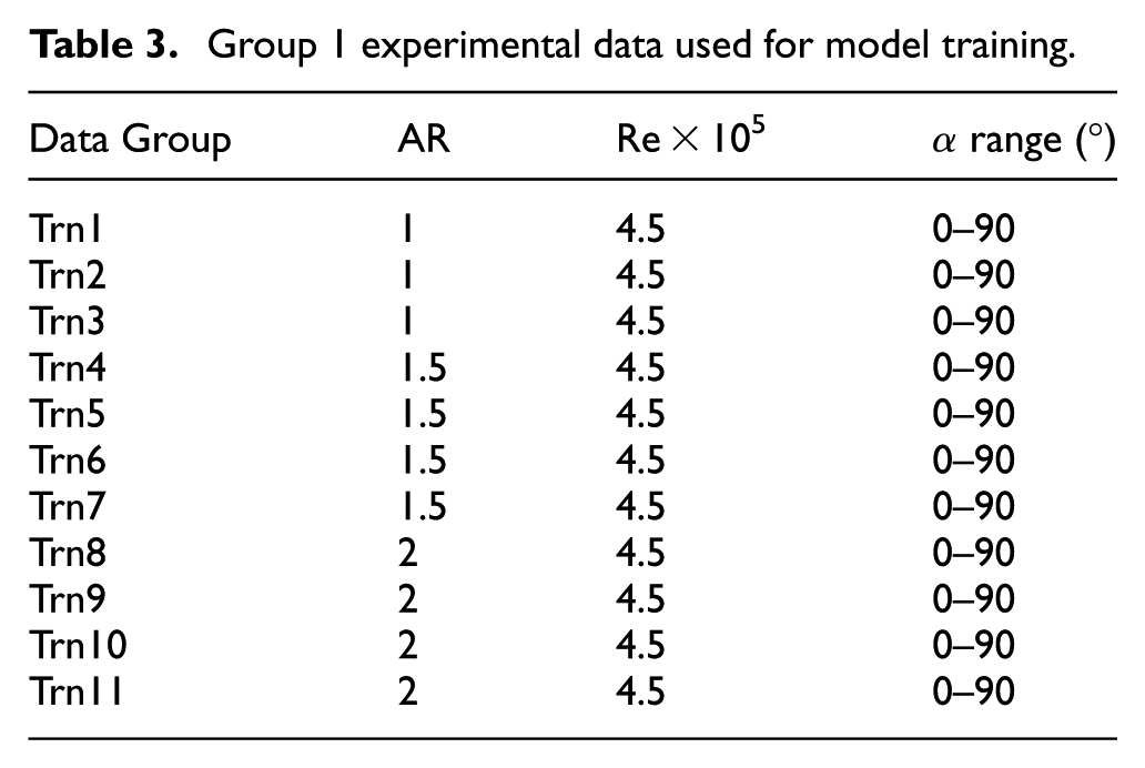
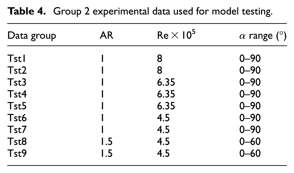
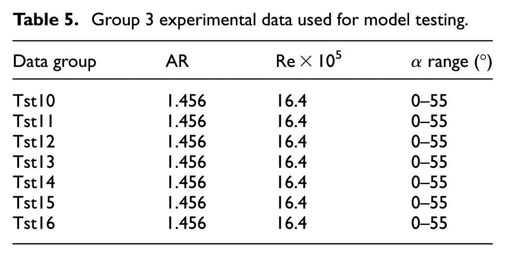
This study aimed to produce an AI model of unsteady aerodynamic loads generated during high-α maneuvering. The NF model predicts aerodynamic loads for a given delta wing by performing a prescribed maneuver. The developed NF model is used to determine the normal force coefficient ( $C_{N}$ ). Experimental data were used to train the NF model, which were primarily the experimental data obtained from unsteady aerodynamic experiments of delta wings performing maneuvers at high angles of attack.²² The experimental data included coefficients of drag ( $C_{D}$ ), lift ( $C_{L}$ ), normal force ( $C_{N}$ ), and pitch moment ( $C_{M}$ ). The outputs from the NF model were compared with those from other experimental and semi-empirical unsteady aerodynamic data.

The developed model was used to estimate aerodynamic coefficients with good accuracy for various maneuvers and wings. In addition, this modeling process was used as a guide for general modeling of similar systems. The model was built and trained based on partial experimental data (group 1; Table 3) obtained.²² The versatility, generality, validity, and accuracy of this model were verified using two groups of experimental data obtained by Jarrah (Table 4, Group 2)²² and Bragg et al. (Table 5, Group 3).²³ Tables 3 to 5 indicate that the data were easily subdivided into various groups to present and clarify the effects of all the inputs and parameters on the model. Using MATLAB, the data were divided³⁷ into training, checking, and testing data, where approximately one of every five points was used as the check point. Figure 3 shows the partitioning of the partial data (Table 3/Group 1) into training and checking points. These data were selected based on availability, simplicity, and representativeness. The K range was represented by values between 0 and 0.06, as listed in Table 2. Some values of K such as 0.02, 0.04 were used to check the overall validity of the model by data subgroups Tst1 to Tst9, as shown in Table 4.

Table 3.

Group 1 experimental data used for model training.

Data Group	AR	Re × 10⁵	α range (°)
Trn1	1	4.5	0–90
Trn2	1	4.5	0–90
Trn3	1	4.5	0–90
Trn4	1.5	4.5	0–90
Trn5	1.5	4.5	0–90
Trn6	1.5	4.5	0–90
Trn7	1.5	4.5	0–90
Trn8	2	4.5	0–90
Trn9	2	4.5	0–90
Trn10	2	4.5	0–90
Trn11	2	4.5	0–90

Table 4.

Group 2 experimental data used for model testing.

Data group	AR	Re × 10⁵	α range (°)
Tst1	1	8	0–90
Tst2	1	8	0–90
Tst3	1	6.35	0–90
Tst4	1	6.35	0–90
Tst5	1	6.35	0–90
Tst6	1	4.5	0–90
Tst7	1	4.5	0–90
Tst8	1.5	4.5	0–60
Tst9	1.5	4.5	0–60

Table 5.

Group 3 experimental data used for model testing.

Data group	AR	Re × 10⁵	α range (°)
Tst10	1.456	16.4	0–55
Tst11	1.456	16.4	0–55
Tst12	1.456	16.4	0–55
Tst13	1.456	16.4	0–55
Tst14	1.456	16.4	0–55
Tst15	1.456	16.4	0–55
Tst16	1.456	16.4	0–55

Figure 3.

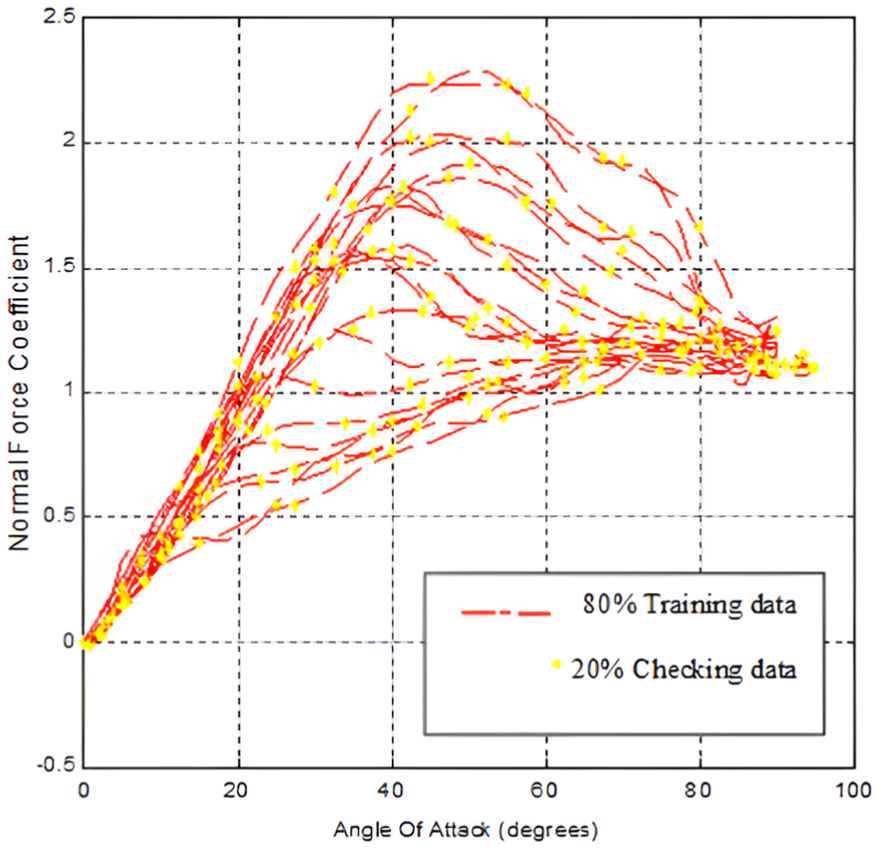
Experimental data partitioning into training and checking data.

Results and discussion

Initial modeling/NF Model 1

The NF modeling process in this investigation started with the simplest model that best fit and tracked the training and checking data with minimal root mean square error (RMSE). RMSE is defined as the average difference between the predicted and actual values produced by a statistical model. It is the residual that stands for the separation between the data points and the regression line. It can be determined by equation¹⁷ as follows:

RMSE = \sqrt{\frac{1}{n} \sum_{i = 1}^{n} {(y_{i} - {\hat{y}}_{i})}^{2}}

(11)

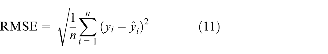
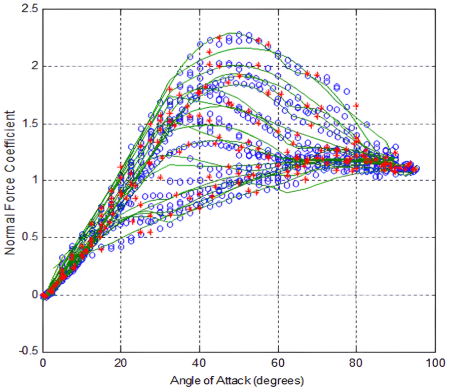
where: n is the number of observations, $y_{i}$ is the observed value, and ${\hat{y}}_{i}$ is the predicted value.

The initial modeling was performed by varying some NF modeling parameters such as the number of MFs, type of MFs, and epoch number. The required MFs best fit the input data in terms of simplicity, convenience, speed, and efficiency. The type and number of MFs were selected by plotting the experimental data and visually dividing the plot into distinct segments. Starting with α, which is the first model input, the experimental data are plotted in Figure 4. The number of MFs for α is set to four; however, the range of the number of MFs for α is considered while fixing the other parameters to justify this choice. The number of MFs for α was 2–9, and the RMSE was found, as illustrated in Figure 5.

Figure 4.

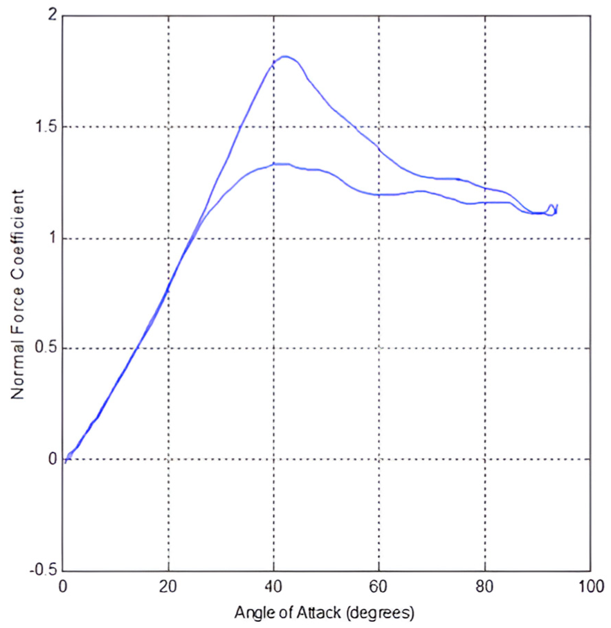
Experimental data at AR = 1 and K = 0.01.

Figure 5.

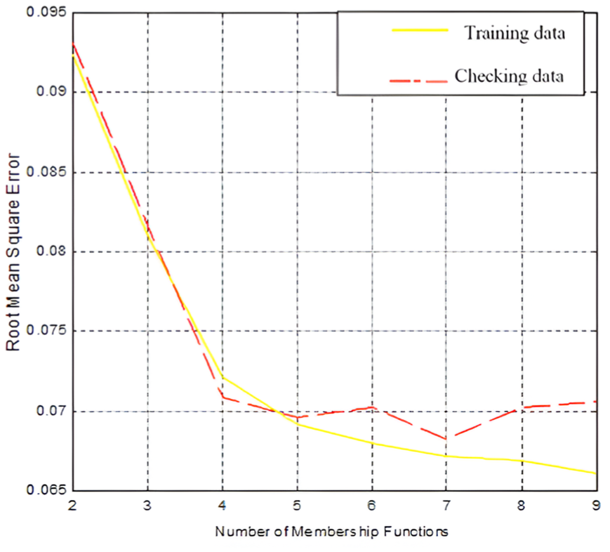
Effect of varying the number of MFs at the angle of attack on prediction accuracy. The number of epoch is 500 and the MF type is Gaussian.

For general training data (Trn1 to Trn 11 as in Table 3), RMSE changed from 9.24% for two MFs to 7.22% for four MF (2.02% difference), whereas it changed to 7.12% for nine MFs (0.1% difference with respect to that for four MFs). The same result was obtained for Group 1 (Figure 3). The optimal number of MFs for α is 4. This is visually evident in Figure 5, where the model complexity when the number of MFs is above four is not associated with a significant RMSE improvement. $\overset{\cdot}{α}$ represents the direction of the maneuver, that is, pitch up and pitch down. Therefore, three or two MFs can be selected as 3 or 2. The number of MFs was varied between 2 and 9 to observe the effect of the choice on the RMSE. The RMSE for general training data changed from 7.22% for two MFs to 3.89% for three MFs, which is a difference of 3.33%. The RMSE was 2.56% for four MFs, with a difference of only 1.33% compared to that for three MFs. Both the training and checking data were equally satisfactory when the number of MFs was three. Subsequently, these data started to deviate, indicating that the accuracy improvement in tracking the training data occurred at the expense of tracking the checked data, thereby adversely affecting the generality of the model. Thus, the most suitable number of MFs was three. Only three MFs can be selected for AR; therefore, the number of MFs should be either two or three. RMSE was 10.59% for 2 MF compared to 7.22% for 3 MF; then, it ceased to change for both general training and checking data; and therefore, the best choice was 3.

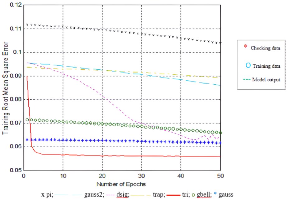
The type of MF was selected by investigating all types of MF, as shown in Figure 1. A comparison of the RMSE values indicated that the effect of the MF type on this model was negligible. The highest RMSE for training data (Trn1 to Trn11) was 7.53% for the triangular MF, and the lowest was 7.01% for both dsig (difference of two sigmoid MF) and trap (trapezoidal) MFs, with a difference of only 0.52%. The triangular MF can be considered to satisfy both the training and checking data equally; therefore, it was selected as the MF type for the initial modeling process (NF Model 1). The RMSE decreases with an increase in the number of epochs, as shown in Figure 6. Therefore, at extremely high epoch numbers, the model rigidly tracked the training data. This adversely affected the prediction of other data outputs, and it was clear that the RMSE decreased significantly from 10.37% at two epochs to 7.22% at 500 epochs. At epoch numbers above 150, the change in the RMSE ceases to be significant.

Figure 6.

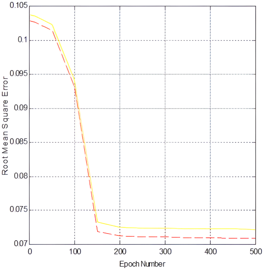
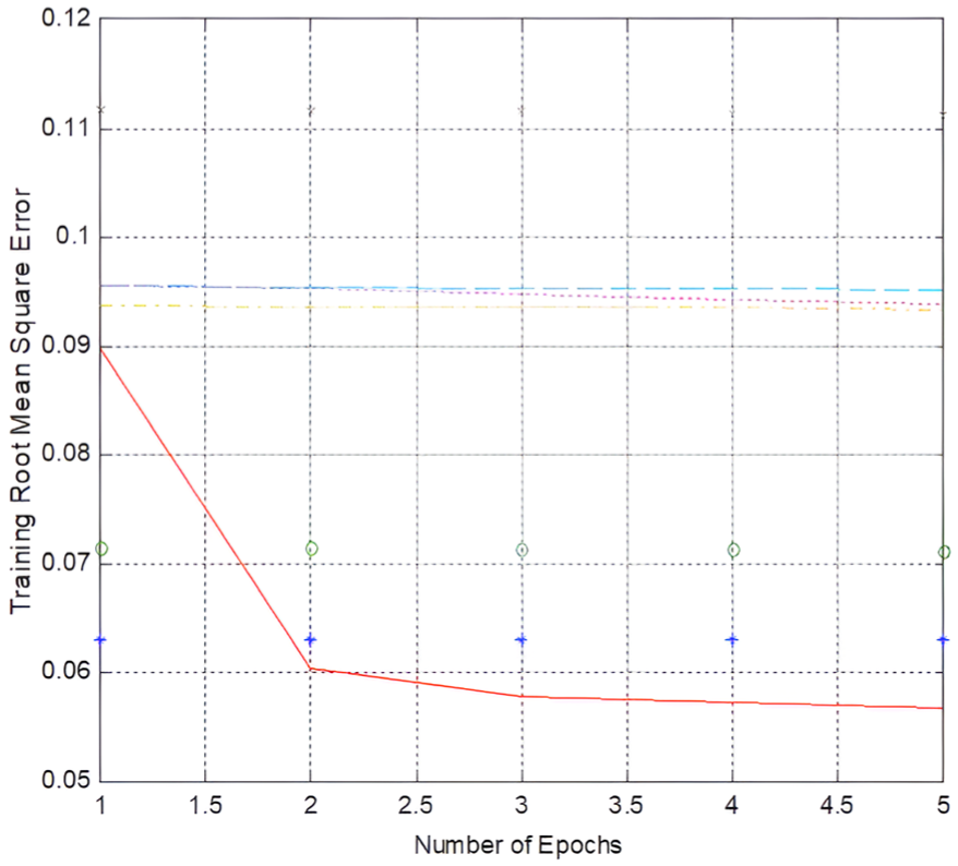
Effect of varying number of epochs on prediction accuracy (MF type is Gaussian, number of MFs are 4, 2, and 3 for $α, \overset{\cdot}{α}, and AR$ , respectively).

The initial model was run with the following parameters to tune the initial modeling to an appropriate number of epochs: triangular MF type; number of MFs = 4, 3, and 3; and number of epochs = 150. Figure 7 shows that the epoch number can be reduced to less than 50 without adversely affecting the RMSE. minimal RMSE at 150 epochs was 5.59% and 5.81% for training and checking data, respectively; the corresponding values at 50 epochs were 5.60% and 5.80%, and those at 5 epochs were 5.68% and 5.80%, respectively. Therefore, considering the RMSE values, the best choice for the epoch number was 5. 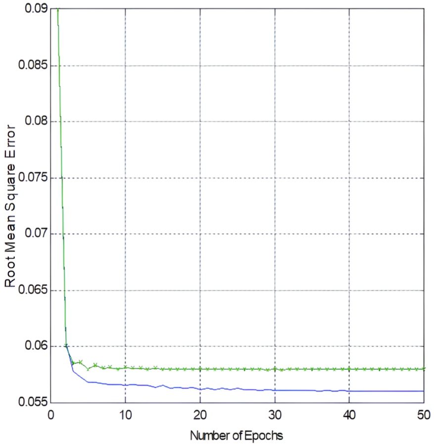Hence, NF Model 1 was set with the following parameters: the type of MF was triangular; the number of MFs was four, three, and three for the three inputs ( $α, \overset{\cdot}{α}, and AR$ ), and the number of epochs was five. This model was achieved while adhereing to the criteria of simplicity, convenience, speed, efficiency, and RMSE values of 5.68% and 5.80% for training and checking data, respectively.

Figure 7.

Error curves at 50 epochs and triangular membership function.

NF Model 1 was the simplest model and provided minimal RMSE for training and checking the data. In other words, it best fits and tracks the local features of the training and checking data plots, while considering simplicity, convenience, speed, accuracy, and efficiency. However, it is necessary to change the rigidity of this model (close tracking of the training data), which can negatively affect the accuracy of predicting other data. This eliminated the need for a general model. This point was monitored through the divergence of the verification data RMSE with respect to the training data RMSE, as shown in Figures 5 to 7. Figure 8 shows the initial MF of NF Model 1, which has the following parameters: the number of MFs is four, three, and three corresponding to $α, \overset{\cdot}{α}, and AR$ , respectively; the MF type is triangular, and the number of epochs is 5. Figure 8 clearly indicates that the initial MFs for each input are equally spaced with sufficient overlap within the input ranges. The final MFs values are shown in Figure 9. No change in the final membership function was observed when the initial and final MFs were compared. In some cases, the final MFs are adjusted to capture the local features of the training data. An example of this case is shown in Figure 10, which was obtained when the number of epochs was changed to 500 and the number of MFs for $\overset{\cdot}{α}$ was set to 2 instead of 3. However, these changes had no positive return on the value of RMSE, which yielded a value of 7.53%; the RMSE of the initial modeling was 5.68%. Therefore, the change in the shapes of the initial and final MFs depends on the combination of the fuzzy model parameters. The various colors of Figures 8 to 10 indicate the number of Membership Functions (MFs) as indicated in the figure caption.

Figure 8.

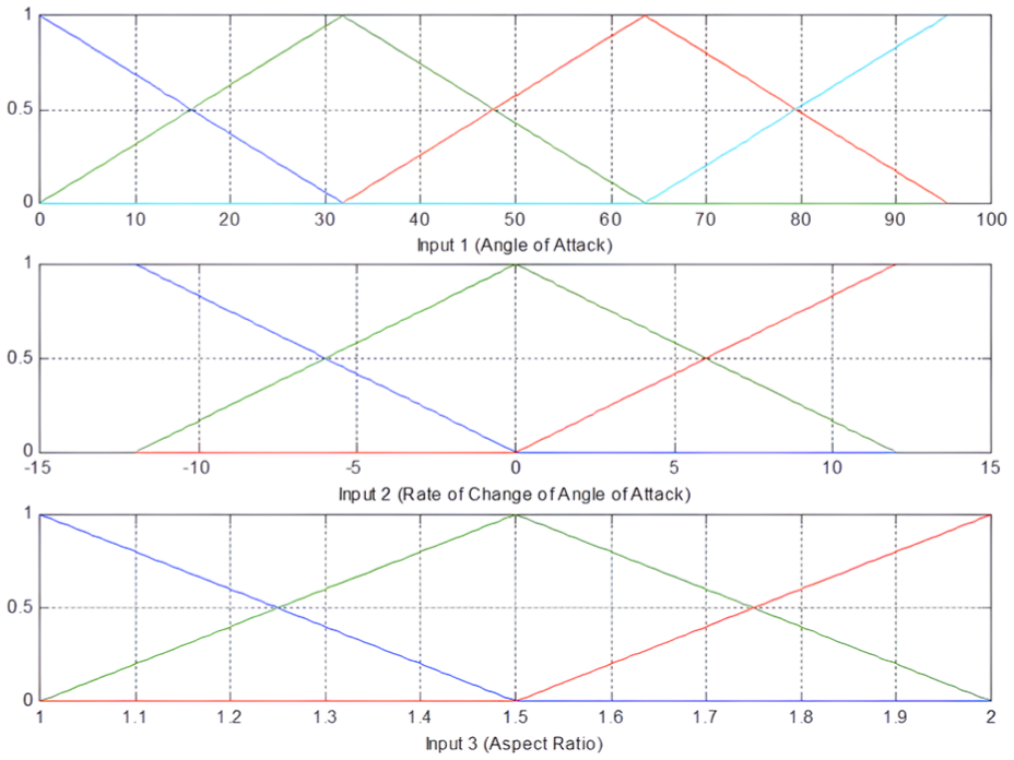
Initial MFs of Model 1 at 5 epochs, number of MFs = [4, 3, and 3], and triangular type MF.

Figure 9.

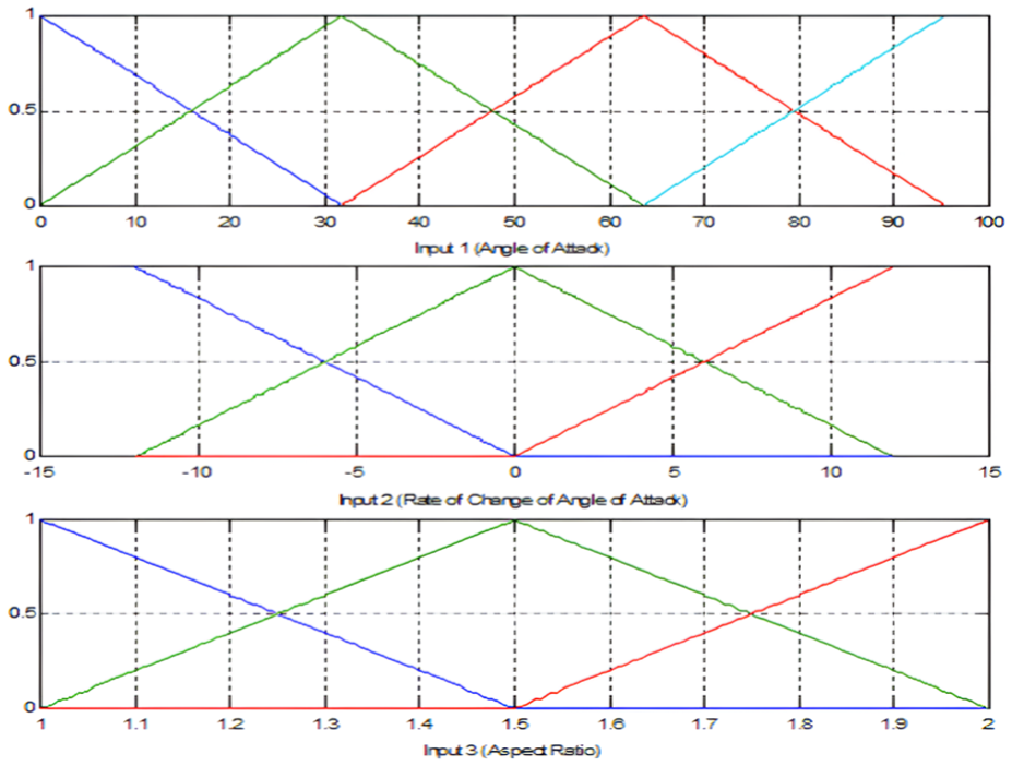
Final MFs of Model 1 at 5 epochs, number of MFs = [4, 3, and 3], and triangular type MF.

Figure 10.

Comparison of $\overset{\cdot}{α}$ initial to final MFs at 500 epochs for 4, 2, and 3 triangular MFs no. = [4 2 3]

Figure 11 shows that the triangular MF has a high rate of convergence compared to other types, where the RMSE goes directly from 8.98% to 6.04% at two epochs, and then to 5.68% at five epochs. The proper selection of the number of MFs is also evident in Figure 12, which represents the initial modeling/NF Model 1 selection of the number of MFs [4, 3, 3], and shows a high rate of convergence of the triangular MF. The outcome of the initial modeling process (NF Model 1) is shown in Figure 13, which reflects the accuracy of this model in predicting the normal force coefficient $C_{N}$ . The general trend of all training and checking data was satisfactory, with an RMSE of less than 6%. However, Figure 13 shows that not all local hysteresis is modeled exactly, particularly at angles of attack above 30°, where the nonlinearity becomes more pronounced. The same comparison was performed for various values of K, AR, and Re, and showed the same trend.

Figure 11.

Convergence comparison for MF types for 4, 3, and 3 MFs for 5 epochs.

Figure 12.

Convergence comparison of MF types for 4, 3, and 3 MFs for 50 epochs.

Figure 13.

Outcome of the initial modeling process (NF Model 1). Number of epochs = 5; Number of MFs = [4 3 3]; and type of MF: triangular.

Examining model generality

One of the most important criteria for any model is the extent of generality, that is, the ability of the model to predict other datasets not used for training or checking (Group1-subgroups Trn1 to Trn11, as in Table 3). To this end, other data (Groups 2 and 3-subgroups Tst1 to Tst16, as in Tables 4 and 5) were used to predict their output using NF Model 1. The need to change the initial modeling/NF Model 1 parameters arises if its rigidity (close tracking of training data) negatively affects the accuracy of predicting other data; therefore, it eliminates the benefit of obtaining a general model. The accuracy and value of NF Models 2 and 3 depended significantly on the accuracy of the experimental data and the degree of matching between the different data groups.

Applying the NF Model 1 parameters to the data in Table 4 revealed that the overall RMSE was 8.35%. In Table 4, the data subgroups Tst1–Tst7 are for $α$ values ranging from 0 °to 90°. In contrast, the Tst8 and Tst9 subgroups were in the $α$ range of 0°–60°, which was not used in designing/training NF Model 1. The lowest RMSE was 4.27% for Tst1 subgroup and the highest was 8.53% for Tst7 subgroup. Higher RMSE values of 19.87% and 14.63% were obtained for Tst8 and Tst9, respectively. The explanation for the high RMSE in the $α$ range of 0°–60° is that all training data were for the $α$ range of 0°–90°. In other words, the model prediction for different $α$ ranges would have been improved if $α_{\max}$ and $α_{\min}$ were used as model inputs and Model 1 was trained for more than one $α$ range. Figure 14 shows a comparison between the output of NF Model 1 and the output using the Group 2 data and Table 4.

Figure 14.

Comparison of NF Model 2/Group 2 data (blue dotted line) to NF Model 1 (Red line).

The previously discussed NF modeling technique was repeated to obtain the simplest model that best fit the data for Group 2 (Table 4). The best choice for the number of MFs of $α$ is four, which agrees with NF Model 1. The number of MFs for $\overset{\cdot}{α}$ is 2 with an RMSE of 7.39%, where it has a value of 19.96% for 3 MFs. This finding agrees with the observation that $\overset{\cdot}{α}$ physically accounts for the maneuver direction. The number of MFs for AR was investigated and found to be three.

The type of MF that best suits Group 2 data was studied and selected to be the Gaussian or triangular type, where RMSE was found to be 7.39% and 7.55%, respectively. However, triangular MF has the advantage of satisfying Groups 1, 2, and 3 equally. The lowest and almost unchanged RMSE were obtained for epoch numbers between 2 and 50 (7.08% at two epochs and 7.09% at 50 epochs). Therefore, the simplest model that best fits the Group 2 data has the following parameters: 4, 2, and 3 MFs; triangular MF; and five epochs (two epochs could have been selected, but five were selected for easier comparison with the parameters of NF Model 1). Therefore, the only difference between the parameters of NF Models 1 and 2 (Group2 data model) is the number of $\overset{\cdot}{α}$ MFs.

NF Model 2 showed a negligible improvement of 8.27% RMSE compared with 8.35% for NF Model 1. The improvement is introduced especially in the subgroups (Tst8 and Tst9), which represent the 0°–60° maneuver. The RMSE for these two subgroups were 17.53% and 11.76%, respectively, with improvements of 2.34% and 2.87% compared to those of the NF Model 1 RMSE. Another improvement was found in subgroup Tst6, with a difference of 0.96%. A negligible improvement was obtained for Tst5 with an RMSE difference of 0.34%. All other subgroups in Table 4 show an increase in the RMSE of less than 2%. A negative effect of Group 2 data on Model 2 training and checking was evident when the training data RMSE was 14.79% compared to 5.68% obtained by Model 1 (a difference of 9.11%). Therefore, the model optimization performed using the Group 2 data in Table 4 does not deviate significantly from the Model 1 parameters. Therefore, NF Model 1 is still more acceptable than NF Model 2 because it satisfies the training, checking, and data requirements listed in Tables 3 and 4.

Similarly, NF Model 3 was built using the experimental data obtained by Bragg et al.¹⁹ as shown in Table 5. Model 1 parameters were tested using the Group 3 data to further enhance the generality of the model (Table 5). Figure 15 shows that Model 2 for $AR$ = 1.5, and $K$ = 0.04, followed by Model 1 for $K$ = 0.02 more closely than Model 3, which had $AR$ = 1.456 and $K$ = 0.0396. Model 3 was expected to be closer to Model 2 because they were both built at $AR$ = 1.5 and $K$ = 0.04. The root mean square difference (RMSD) between Models 1 and 2 was 10.06%, and which increased to 16.02% for Models 2 and 3, both of which had approximately the same nondimensional pitch rate and AR. Therefore, the effect of the difference in the procedures of the two experiments^22,23 overcomes the effect of the major parameters, that is, the AR and non-dimensional pitch rate.

Figure 15.

Comparison of Model 3 (AR = 1.456 & K = 0.0396, green solid line) to Model 2 (AR = 1.5 & K = 0.04, blue line) and Model 1 (AR = 1.5 & K = 0.02, red line).

Model 1 parameters were used to predict the data from Bragg et al. (Table 5). The results are shown in Figure 16. The highest RMSE was 83.61% for the Tst15 subgroup and the lowest was 18.41% for the Tst10 subgroup. Both are considered high, which can be attributed to the differences in the procedures of the two experiments,^22,23 as discussed in Section IV. The best model that fits the Group 3 data was investigated to further check whether the problem is with model selection or the differences in the two experiments (applying the same NF Model tuning procedure, the simplest model that best fits the Group 3 data was found and named NF Model 3). The investigation revealed that Model 3 had the following parameters: the number of MFs was two, two, and two for α, AR, $and \overset{\cdot}{α}$ , respectively; the type of MF was dsig; and the number of epochs was five. The lowest RMSE for Model 3 was 13.72%, the highest was 20.69%, and both were considered to be high. Model 3 adversely affected the NF modeling of all other data groups. Another reason for the high RMSE, in addition to the differences in the experimental procedures, is that Bragg et al.’s²³ data have a 0°–55°α range, whereas Models 1 and 2 were trained using a 0°–90°α range only.

Figure 16.

Modeling Group 3 data by NF Model 3 (blue dotted line) and NF Model 1 (red solid line). K = 0.0072, AR = 1.456, and Re = 16.4 × 10⁵.

Accuracy analysis of the final NF model (Model 4)

Based on the analysis carried out previously, the final NF model (Model 4) best fit the training and checking data from Group 1 (Table 3) and Group 2 (Table 4), except for subgroups Tst8 and Tst9, owing to the difference in the α ranges. $α_{\max}$ and $α_{\min}$ must be included in the model inputs if different α ranges are predicted. Model 4 had a normal force coefficient as its output and three inputs (α, AR, and $\overset{\cdot}{α}$ ). The corresponding numbers of MFs were four, three, and three; the MF type was triangular for all three inputs, and there were five epochs. The modeling accuracy exhibited a varied dependency on α, AR, and $\overset{\cdot}{α}$ . In addition, the variation depends on the individual model inputs, and it was found that the model is more sensitive to the selection of the number of MFs for $\overset{\cdot}{α}$ than for α, which depends on the physical and mathematical nature of the target system being investigated, and on the number of experimental points for each input. Investigating the effect of varying number of MFs for α showed that the RMSE ranged from a minimum value of 6.61% at 9 MF to a maximum of 9.24% for two MFs with a difference of 2.63%. The same investigation was conducted for $\overset{\cdot}{α}$ , where the minimum RMSE for the total training data was 1.41% for nine MFs, while the maximum was 7.22% for two MFs, which is a difference of 5.81%. When this was investigated for AR, the difference in the RMSE was 3.37%.

Although the RMSE difference based on the selection of number of MFs was as high as 5.81%, the difference in RMSE for the total training data caused by variations in the MF type was only 0.52%. epoch number selection produced an RMSE difference of 3.15% for the total training data from two to 500 epochs. The last three percentages automatically arranged the model sensitivity to parameter selection as follows: highly sensitive to the MF number, less sensitive to the epoch number, and negligibly sensitive to the MF type. Once the appropriate model parameters were selected, the RMSE converged rapidly in a very small number of epochs: 5.68% RMSE was reached at 5 epochs, 7.33% at 150 epochs, and 7.22% at 500 epochs. The accuracy of NF modeling depends significantly on the accuracy of the experimental data used for training. However, the errors (high RMSE) in this NF model are attributed to variations in the experimental data used for training and comparing the various NF model predictions. This is valid for both experiments,^22,23 where they have different experimental procedures. The two experiments varied in terms of tare measurements, data filtering, data acquisition, variable definitions (such as $K$ , angle-of-attack ranges, and experimental settings. Modeling enhancements can be achieved by increasing the experimental data used for training, particularly for angles of attack ranging from 0° to 60°. Furthermore, an improvement can be achieved in the output prediction of the 0°−60°α range if the model sensitivity to $\overset{\cdot}{α}$ is reduced by reducing its MF number and considering both $α_{\max}$ and $α_{\min}$ as model inputs.

Comparison with semi-empirical data

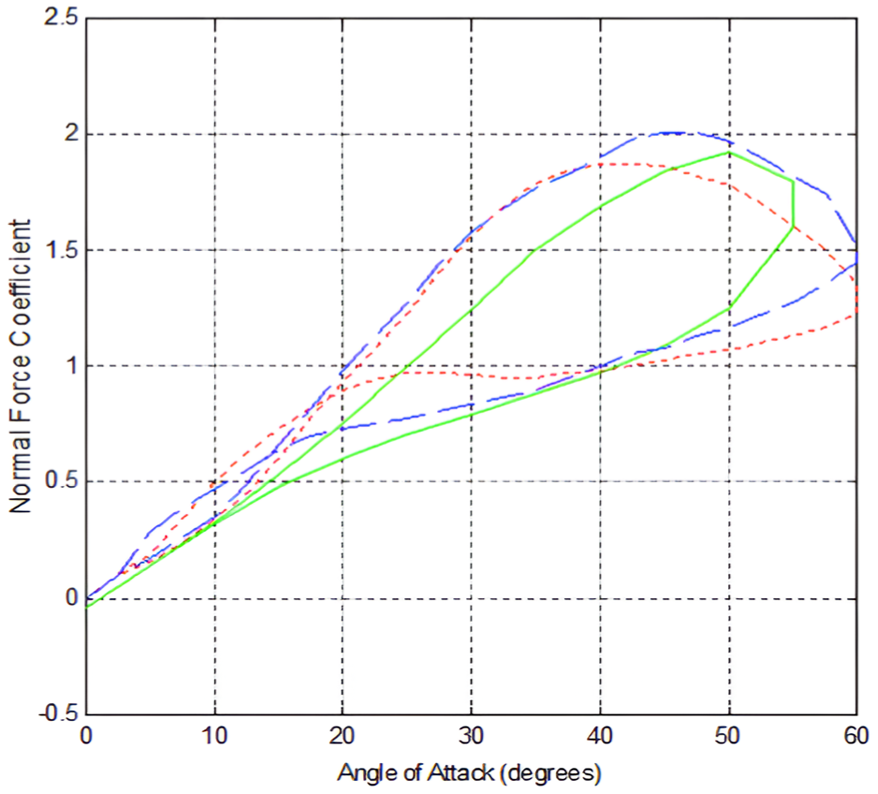
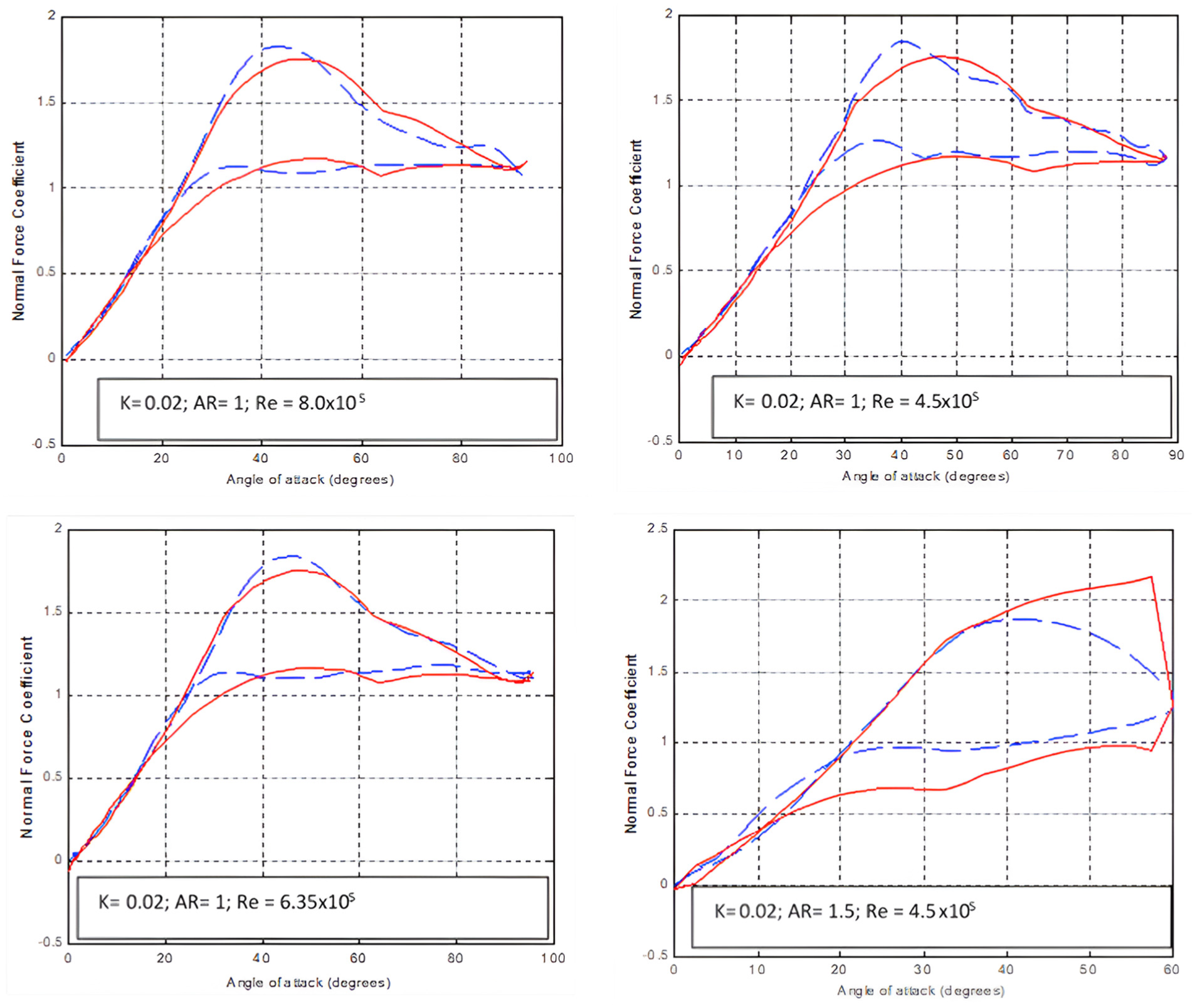
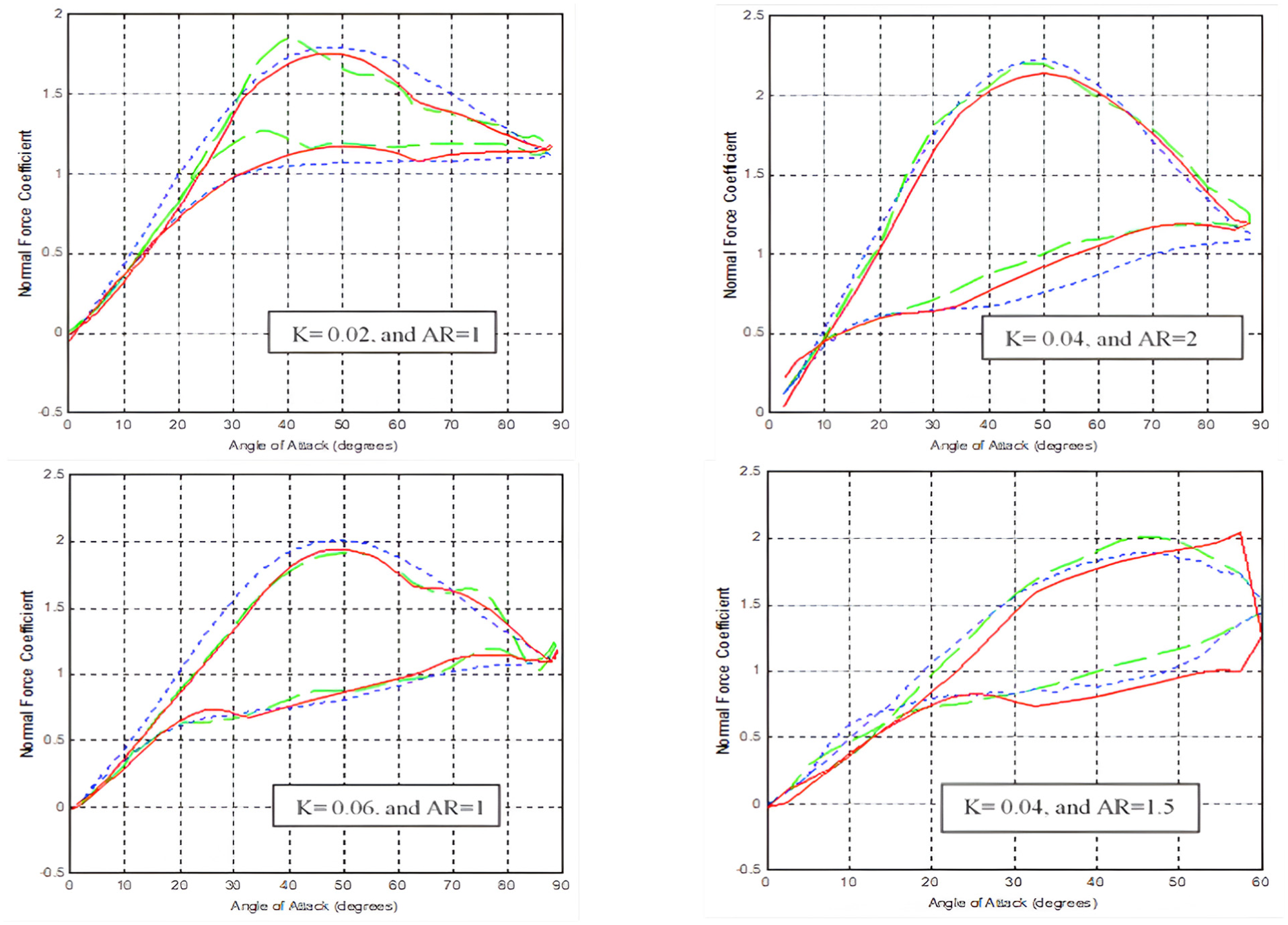
The normal force coefficient predicted using the semi-empirical method was obtained from Ref.³⁸ Figure 17 shows the normal force coefficient obtained by the three methods, that is, Jarrah experiment,²² semi-empirical method,³¹ and NF model established in this research. Table 6 shows a comparison between the semi-empirical and NF models based on the RMSE. For AR = 1 and $K$ = 0.02, Figure 17 shows that the NF model tracked the experimental data more closely than the semi-empirical data. This is the case over the entire angle-of-attack range, except for a very small range of the maximum normal force coefficient. For AR = 1 and $K$ = 0.06, a similar trend was observed, with noticeably improved tracking during pitch-down for both the semi-empirical and NF outputs. For $K$ = 0.06, Figure 17 presents a more pronounced comparison in favor of NF modeling. For the 0°–60°α range, the semi-empirical method yielded a slightly better prediction than NF modeling. The lower accuracy in NF modeling was attributed to training using only a 0°–90°α range and not using $α_{\max}$ and $α_{\min}$ as the NF model inputs. The largest deviation in the NF model prediction occurred in the region with maximum α. This is a reasonable result because the model was trained for a maximum α of 90°, whereas the maximum angle required for the prediction was 60°. For $AR$ = 2 and $K$ = 0.04, NF modeling yielded an improved prediction over the semi-empirical method.

Figure 17.

Comparison of semi-empirical (blue line) NF model (red line) and experiment in Ref.²² (green line).

Table 6.

Comparison of semi-empirical ³ and investigated NF model.

Model parameters Reynolds number = 4.5 × 10⁵			Percent root mean square error (% RMSE)
Aspect ratio	Non-dimensional pitch rate	A range (°)	Fuzzy final model	Semi-empirical method
1	0.02	0–90	8.26	11.12
1	0.04	0–90	8.53	9.18
1	0.06	0–90	4.57	9.92
1.5	0.04	0–60	14.63	8.1
2	0.04	0–90	6.94	11.76
2	0.06	0–90	5.47	17.28
1&2	Range above	0–90	6.75	11.85
Range above	Range above	Ranges above	8.17	12.37

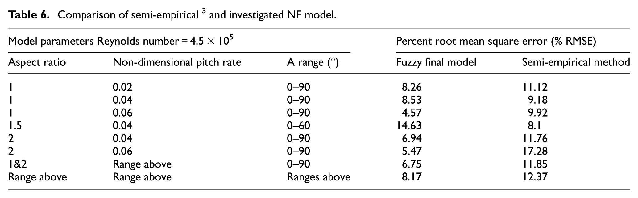
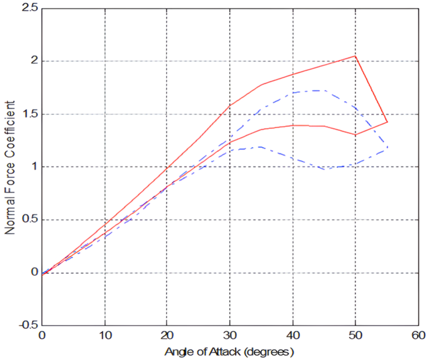
Figure 18 was constructed with the same values as those in Figure 17 and added to the corresponding Bragg et al. data.¹⁹ Bragg et al.’s data deviated from Jarrah’s data²² during the pitch-up motion. The RMSD between Jarrah experimental data and the corresponding values obtained by the semi-empirical method was 8.10%. For the NF data, it was 14.63%, whereas for Bragg et al.’s data, it was 15.36%. This can be attributed to Jarrah’s experimental procedure, wherein the parameter definitions differed from those used in Bragg et al.’s experiment. Therefore, the comparison favors NF modeling for all input ranges, except for the 0°–60°α range. This is attributed to the NF model being trained based only on the 0°–90°α range and without considering $α_{\max}$ and $α_{\min}$ as model inputs.

Figure 18.

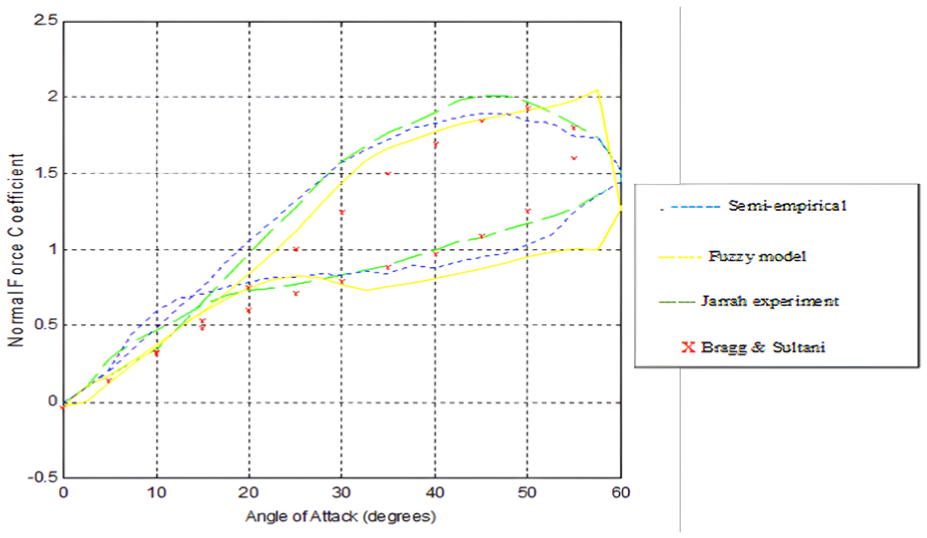
Comparison of semi-empirical, NF model, Jarrah experiment (K = 0.04, AR = 1.5), and Bragg et al. (K = 0.0396, AR = 1.456).

The unsteady aerodynamic coefficients were $C_{N}$ , $C_{L}$ , $C_{D}$ , $C_{M}$ , $C_{RM}$ . In this study, the normal force coefficient ( $C_{N}$ ) was investigated as a model output because experimental data are available from different sources^22,23,38 for modeling and comparison. A similar modeling procedure can be used to model any other coefficient. Three NF modeling inputs were selected by studying the effect of aerodynamic variables on coefficients $α$ , $\overset{\cdot}{α}$ , and $AR$ . These were the most significant parameters affecting the aerodynamic loading. The NF modeling parameters investigated to obtain the optimum model included the number of MFs for each input, type of MF, and number of epochs. The available experimental data²² were partitioned into 80% training data and 20% verification data, to ensure simplicity, availability, and representation. Only the angles of attack ranging from 0 °to 90° were used to train and verify the NF model. The non-dimensional pitch rate ( $K$ ) values were taken as 0, 0.01, 0.03, and 0.06, and other available values were used to prove the ability of the model to predict data in addition to the training data. Three ARs (1,1.5, and 2) and several MFs were used; however, the best model was obtained with four, three, and three MFs for the $α$ , $\overset{\cdot}{α}$ , and $AR$ models, respectively. The RMSE was used as a measure of acceptable accuracy, and the number of MFs was approximated by plotting the experimental data and dividing the figure into distinct segments. The choice of four MFs for $α$ was selected because four cases were recognized.

1) Low α where the flow is attached or separated but organized.

2) High α where the vortical flow dominates the flow field.

3) An extremely high α is characterized by the breakdown of the vortex and flow structure, an increase in separation drag, and loss of lift.

4) The flow field was characterized by strong wake vortices, where the lift was near zero, and the normal forces on the wing were attributed to those caused by the cross-flow drag.

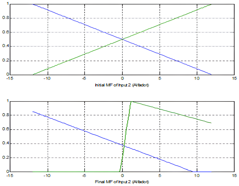
Aerodynamic experiments and analyses^22,23 showed that there are three distinct cases of $\overset{\cdot}{α}$ . The value can be zero (static or steady). The second case had a negative value (pitch-down motion), and the third case had a positive value (pitch-up motion). Seven MF types were investigated in this study. The MF type had a negligible effect on the modeling of the system; therefore, the simplest one (triangular) was set as the primary modeling MF type and was found to satisfy the training and checking data equally.

The smallest number of epochs is desired because it is simple and saves time; however, this requirement was considered the second priority after the high model prediction accuracy. It was found that five epochs were the most suitable because they provided an RMSE of 5.68% compared to that of 5.6% at 50 epochs, which is a very small improvement. Adapting the initial model (Model 1) to predict the training and checking data yields RMSE values of 5.68% and 5.8%, respectively, which are considered to be excellent values. The resulting initial and final MF had no significant positive effects on model prediction. For NF Model 1, the initial and final MF shapes were identical. The following model parameters were selected: MF number = [4 2 3], the MF type was triangular, and the number of epochs was 500. The initial and final MF shapes for $\overset{\cdot}{α}$ were different. RMSE increased to 7.53% compared with 5.68% obtained using the initial model.

Model generality was checked by predicting the Group 2 data and Table 4, which were not used for training. NF Model 1 predicted the data with an overall RMSE of 8.35%. The lowest RMSE was 4.27% for the subgroup with $K$ = 0.01, $AR$ = 1, and an $α$ range of 0°–90°. The highest was 19.87% for the data group with an $α$ range of 0°–60° and K = 0.02. Table 4 shows that subgroups that have $α$ ranges of 0°–90° had RMSE values of less than 10%. NF Model 2 was obtained using data from Table 4 and had the following parameters: MF number of [4 2 3], triangular MF type, and five epochs. This model did not appreciably improve the prediction of Table 4, where the overall RMSE was 8.27% compared with 8.35% for Model 1. Therefore, Model 1 was proven to be optimal, even for data other than those used for the training.

Bragg et al.’s data²³ (Table 5) were predicted using NF Model 1. The RMSE for all of Bragg et al.’s data (Table 5) was high (43.47%), and a model particularly optimized for Bragg et al.’s data (Model 3) was found, yielding an RMSE of 16.49%. The high RMSE was explained by the differences in the experimental procedures for both the experiments.^22,23

Therefore, the best NF model, named the final model (Model 4), was set with the same parameters as those in Model 1. Implementing the NF Model 4 yielded an RMSE of 5.68% for Group 1/Table 3 training data and 8.35% for Group 2/Table 4. comparison with the semi-empirical method³⁶ revealed NF modeling for all data groups except for the 0°−60° $α$ range, where RMSE values were 14.63% and 8.1% for NF and semi-empirical methods, respectively. The overall RMSE values for the 0°–90° $α$ range were found to be 6.75% for the NF model and 11.85% for the semi-empirical methods. In addition, the NF model is more favorable than the semiempirical method. For $K$ = 0.02, 0.04, and 0.06, and $AR$ = 1 and 2 in the 0°–90°α range, the average RMSE was found to be 6.75% for the former and 11.85% for the latter.

Conclusion

In this study, an NF model was developed to predict the normal force coefficient with an overall root mean square error (RMSE) of less than 6% for angles of attack (α) ranging from 0° to 90° and less than 20% for the 0° to 60° range. The model can give even lower RMSE, but this may cause unnecessary increased model complexity. For instance, the optimal number of membership functions (MFs) was found to be four, suggesting that increasing complexity does not necessarily enhance performance significantly beyond the 6% RMSE. Data groups with input ranges matching those used for training exhibited lower RMSE. The model can be easily adapted to predict similar linear and nonlinear systems, including steady and unsteady aerodynamic coefficients. The accuracy of the model is significantly influenced by the number of membership functions (MFs) selected, though it shows lower sensitivity to the type of MF used. Once appropriate model parameters are chosen, the RMSE converges rapidly with a small number of epochs. Model accuracy is most affected by the rate of change in α and aspect ratio (AR), followed by α itself.

The NF models compared favorably with semi-empirical methods for an α range of 0° to 90°, but the semi-empirical method was more accurate for the 0° to 60° range. This discrepancy is likely because α_min and α_max were not included as model inputs, and only the 0° to 90° range was used to train the NF model. Enhancing the model involves increasing the size of the experimental dataset used for training and validation. For better modeling and prediction of unsteady aerodynamic loads across different α ranges, incorporating α_min and α_max as model inputs is necessary. Model accuracy depends on three key parameters: the number of MFs, the type of MF, and the number of epochs. With the correct parameters, the RMSE converges quickly with minimal epochs.

Training should encompass multiple α ranges, with data for at least five ranges used, including low to moderate (0°–30°), low to high (0°–60°), and low to extremely high (0°–90°), along with two other ranges with different minimum values. Future work should aim to improve the modeling of local hysteresis, particularly at angles above 30°, where nonlinearity is dominant. Additionally, the modeling procedure should be extended to predict all five unsteady aerodynamic coefficients, not just the normal force coefficient. While this study used the Sugeno scheme for NF modeling, further research should explore the Mamdani method.

The developed model gives evidence that neuro-fuzzy techniques are very valuable in modeling unsteady aerodynamic. However, future work will include additional machine learning teachings with more data obtained for other aircraft. Future work will include exploration of hybrid approaches including combining neuro-fuzzy techniques with other machine learning models. This will enhance the robustness and effectiveness of the model. Future work will also include more aerodynamic data relevant to other aircraft to further enhance the modeling process

Footnotes

Acknowledgements

We thank Rabdan Academy (RA) and Higher Colleges of Technology (HCT) for supporting this work.

ORCID iD

Mohammad Almajali

Ethical considerations

This work did not involve humans or animals. Ethical approval was not required for this research.

Consent for publication

The corresponding author gave consent to participate in the publication of the identifiable details.

Author contributions

Aziz Almahadin collected the data for this work, carried out the conception and design, analyzed and interpreted the data, and drafted the manuscript. Mohammad Almajali supervised the study, revised the manuscript critically for intellectual content, participated in the design, and drafted the final version to be published. All authors read and approved the final draft and agree to be accountable for all aspects of the work.

Funding

The authors received no financial support for the research, authorship, and/or publication of this article.

Declaration of conflicting interests

The authors declared no potential conflicts of interest with respect to the research, authorship, and/or publication of this article.

Data availability statement

The data and materials supporting the results or analyses presented in this paper are available upon reasonable request.

References

Zore

Matyushenko

Shah

, et al. Laminar–turbulent transition prediction on industrial computational fluid dynamics applications. J Aircr 2023; 60(1): 1–20.

Nguyen

Ogburn

Gilbert

, et al. Simulator study of stall/post stall characteristics of a fighter airplane with relaxed longitudinal static stability, NASA TP 1538. NASA Technical Reports Server, 1979.

Nguyen

Goman

Lowenberg

, et al. Evaluation of unsteady aerodynamic effects in stall region for a T-tail transport model. In: AIAA SciTech Forum, San Diego, CA, 2022.

Linse

The design and analysis of high angle of attack fighter control system. University of Kansas Flight Research Laboratory, Rept. KU-FRL-776-1, Lawrence, KS, 1987.

Gratton

Reduced-order, trajectory piecewise-linear models for nonlinear computational fluid dynamics. Massachusetts Institute of Technology, 2004.

Ghoreyshi

Jirásek

Cummings

RM.

Reduced order unsteady aerodynamic modeling for stability and control analysis using computational fluid dynamics. Prog Aerosp Sci 2014; 71: 167–217.

Luchtenburg

Rowley

Lohry

, et al. Unsteady high-angle-of-attack aerodynamic models of a generic jet transport. J Aircr 2015; 52(3): 890–895.

Imamguluyev

Umarova

. Application of fuzzy logic apparatus to solve the problem of spatial selection in architectural-Design Projects. In: Kahraman

Cebi

Cevik Onar

, et al. (eds) Intelligent and fuzzy techniques for emerging conditions and digital transformation. INFUS 2021. Lecture Notes in Networks and Systems. Springer, 2022, Vol. 307, pp. 842–848.

Aslan

Altan

Hacıoğlu

. Level control of blast furnace gas cleaning tank system with fuzzy based gain regulation for model reference adaptive controller. Processes 2022; 10(12): 2503.

10.

Tekin

Cebi

Kaya

. Retention prediction in the gaming industry: fuzzy machine learning approach. In: Calisir

(ed.) Industrial engineering in the age of business intelligence. GJCIE 2021. Lecture Notes in Management and Industrial Engineering. Springer, 2023, pp. 87–96.

11.

Zhang

Jiang

Yang

, et al. Federated transfer learning for remaining useful life prediction in prognostics with data privacy. Meas Sci Technol 2025; 36: 076107.

12.

Al-Mahadin

Papageorgiou

. Investigating the Appropriateness of fuzzy logic techniques to model unsteady aerodynamics. In: Advances in Science and Engineering Technology International Conferences (ASET), Dubai, 2020.

13.

Talpur

Abdulkadir

Alhussian

, et al. Deep Neuro-Fuzzy System application trends, challenges, and future perspectives: a systematic survey. Artif Intell Rev 2023; 56: 865–913.

14.

Tumse

Bilgili

Sekertekin

, et al. Comparison and evaluation of machine learning approaches for estimating heat index map in Türkiye. Neural Comput Appl 2023; 35(21): 15721–15742.

15.

Wang

Lan

Brandon

. Fuzzy logic modeling of nonlinear unsteady aerodynamics. 1998. DOI:10.2514/6.1998-4351.

16.

Liu

Sun

Jiang

, et al. Fuzzy logic modeling of nonlinear unsteady aerodynamics. AIAAA J 2005; 19: 99–103.

17.

Zhang

Han

Zhang

, et al. Unsteady aerodynamic identification based on recurrent neural networks. J Vibroengineering 2021; 23(2): 449–458.

18.

Song

Bai

GC.

Vectorial surrogate modeling approach for multi-failure correlated probabilistic evaluation of turbine rotor. Eng Comput 2023; 39: 1885–1904.

19.

Pradhan

Jena

Talukdar

, et al. A new method to evaluate gold mineralisation-potential mapping using deep learning and an explainable artificial intelligence (XAI) model. Remote Sens 2022; 14: 4486.

20.

Song

Zhu

, et al. Cascade ensemble learning for multi-level reliability evaluation. Aerosp Sci Technol 2024; 148: 109101.

21.

Garud

Jayaraj

Lee

A review on modeling of solar photovoltaic systems using artificial neural networks, fuzzy logic, genetic algorithm and hybrid models. Int J Energy Res 2021; 45(1): 6–35.

22.

Jarrah

MA.

Unsteady aerodynamics of delta wings performing maneuvers at high angle of attack. Department of Aeronautics and Astronautics, Stanford University, 1988.

23.

Bragg

Sultani

Brandon

JM.

Experimental measurements on an oscillating 70-degree delta wing in subsonic flow. Report No. AIAA Paper 88–2576, 1990.

24.

Ericsson

. Dynamic omnipresence of moving wall effects, a selective review. In: AIAA Paper 87-0241, 2012.

25.

Smith

JHB

. Theoretical modelling of three-dimensional vortex flows in aerodynamics. Aeronaut J 2016; 88(874): 101–116.

26.

Tumse

Bilgili

Sahin

Estimation of aerodynamic coefficients of a non-slender delta wing under ground effect using artificial intelligence techniques. Neural Comput Appl 2022; 34: 10823–10844.

27.

Zhang

Yang

, et al. Data-driven deep learning approach for thrust prediction of solid rocket motors. Measurement 2024; 225: 114051. https://ssrn.com/abstract=4564471

28.

Tümse

İlhan

Bilgili

, et al. Estimation of wind turbine output power using soft computing models. Energy Sour Part A: Recov Utilization Environ Effects 2022; 44(2): 3757–3786.

29.

Zadeh

LA.

Fuzzy sets, fuzzy logic, and fuzzy systems: selected papers by Lotfi A Zadeh. In: Klir

Yuan

(eds) Advances in fuzzy systems-applications and theory. WSPC, 1996, 1st ed, p. 840.

30.

Makkar

Application of fuzzy logic: a literature review. Int J Stat Appl Math 2018; 3(1): 357–359.

31.

Simon

Sum normal optimization of fuzzy membership functions. Int J Uncertain Fuzziness Knowl Based Syst 2002; 10(04): 363–384.

32.

Sadollah

Introductory chapter: which membership function is appropriate in fuzzy system. In: Sadollah

(ed.) Fuzzy logic based in optimization methods and control systems and its applications. IntechOpen, 2018.

33.

Nguyen

Prasad

NR.

Fuzzy modeling and control: selected works of Sugeno. CRC Press, 1999.

34.

Kluska

Analytical methods in fuzzy modeling and control. Springer Science & Business Media, 2009.

35.

Mohd Adnan

MRH

Sarkheyli

Mohd Zain

, et al. Fuzzy logic for modeling machining process: a review. Artif Intell Rev 2015; 43(3): 345–379.

36.

Karaboga

Kaya

Adaptive network based fuzzy inference system (ANFIS) training approaches: a comprehensive survey. Artif Intell Rev 2019; 52(4): 2263–2293.

37.

Taskin

Kumbasar

. An open source matlab/simulink toolbox for interval type-2 fuzzy logic systems. In: IEEE symposium series on computational intelligence, Cape Town, South Africa, 2015.

38.

Jarrah

MA.

Prediction of unsteady aerodynamic forces on maneuvering delta wings. J Fluid Struct 1995; 9: 925–936.

Artificial intelligence-neuro fuzzy method for modeling the unsteady aerodynamics of an aircraft

Abstract

Keywords

Introduction

Mathematical model

Jarrah’s experiment

Bragg’s experiment

Results and discussion

Initial modeling/NF Model 1

Examining model generality

Accuracy analysis of the final NF model (Model 4)

Comparison with semi-empirical data

Conclusion

Footnotes

Acknowledgements

ORCID iD

Ethical considerations

Consent for publication

Author contributions

Funding

Declaration of conflicting interests

Data availability statement

References