
Abstract
This article is aimed to propose a simple yet efficient unified numerical strategy for solving both linear and non-linear optimal control problems. To do so, the general form of quadratic performance index function and nonlinear state equations are considered first. Then, the idea of variational differential quadrature method is used to convert the integral/differential equations to the equivalent algebraic form. Since time is the only independent variable is this research, the finite difference method with an equally-spaced discretization scheme would be a more appropriate technique rather than the differential quadrature approach. So, the implemented numerical solution is called now as the variational finite difference method. The method of Lagrange multipliers is then utilized for minimization purpose and, as a result, the final set of nonlinear algebraic equations are obtained. Finally, the quadratic and triadic forms of non-linearity are considered and an explicit formulation is represented for the residual and Jacobian of the Newton-based iterative solution procedure. To demonstrate the accuracy and efficiency of the proposed approach in the quadratic optimal control area, several benchmark problems involving linear time-invariant, linear time-variant and nonlinear examples are successfully solved and the results are confirmed with those existed in the literature.
Introduction
Optimal control is an active research area in the control theory with several multi-disciplinary applications. It is used in various fields including bioengineering, economics, robotics, management, process control, finance, aerospace and communication networks.1–3 The well-known theories of linear-quadratic and Gaussian optimal control are dated back to 1960s represented by Kalman. 4 The optimal control theory is mainly utilized to transfer the system to the final desired situation by minimizing an objective function and satisfying certain conditions.
Many researchers have addressed various optimal control problems, and several solution approaches have been proposed in their works. Generally speaking, the reason of enormous attempts is the difficulty of developing an efficient solution technique to find the optimum value of a cost function (in integral form) subjected to the nonlinear state equations (in differential form) and certain boundary conditions (in algebraic form). Tsai et al. 5 developed an approach to design an optimal digital regulator for continuous-time two-dimensional systems described by linear partial differential equations (PDEs). A new state vector was introduced to directly convert the original continuous-time two-dimensional quadratic cost function into a decoupled discretized form. A numerical method was developed by Jaddu 6 to solve nonlinear optimal control problems with terminal state constraints, control inequality constraints and simple bounds on the state variables. Huang and Li 7 used the conjugate gradient method with adjoint equation to solve a general three-dimensional optimal boundary control problem with the aim of determining the optimal boundary control functions. Gerdts et al. 8 studied optimal control problems for the wave equation. To accomplish this aim, they employed a full discretization method based upon finite differences through which the PDE constrained optimal control problem is transformed into a nonlinear programming problem. On the other hand, Tricaud and Chen 9 proposed a numerical approximate method to solve fractional-order optimal control problems in general form. Casas and Tröltzsch 10 analyzed a distributed optimal control problem governed by a quasilinear elliptic equation of non-monotone type using a numerical approach. Yousefi et al. 11 suggested an approximate solution for the fractional optimal control problems by using the Legendre multiwavelet in conjunction with the collocation method. Also, state-constrained optimal control problems for PDEs were numerically analyzed by Neitzel and Tröltzsch. 12 Based on interpolating scaling functions, Foroozandeh and Shamsi 13 presented a numerical approach to solve nonlinear optimal control problems including state and control inequality constraints. Kammann et al. 14 presented a posteriori error estimation for semilinear parabolic optimal control problems with application to model reduction by proper orthogonal decomposition (POD). Bhrawy et al. 15 utilized the shifted Legendre orthogonal polynomials to numerically solve the multi-dimensional fractional optimal control problem with a quadratic performance index.
More recently, by employing the Ritz method, Mamehrashi and Yousefi 16 obtained numerical solution for a class of two-dimensional quadratic optimal control problems. Keshavarz et al. 17 derived a general formulation for the Bernoulli operational matrix of fractional order integration and multiplication. Mamehrashi and Yousefi 18 also presented a numerical solution approach based upon shifted Legendre polynomials for solving a nonlinear two-dimensional optimal control problem. Furthermore, based on the combination of epsilon penalty and variational methods, Lotfi 19 developed an approximate method to address a class of multidimensional fractional optimal control problems. Bourdin and Trélat 20 perused the linear-quadratic optimal sampled-data control problems. The system under consideration involves the continuous state variables and piecewise constant control in time. Also, Chen et al. 21 presented an investigation on the system identification and control of convex problems by respectively employing the neural networks and optimal controller design. Hajiloo et al. 22 presented a multi-objective optimization approach for Pareto optimum design of robust integer-order and fractional-order PID controllers for both integer-order and fractional-order plants with parametric uncertainties. Yıldırım Aksoy et al. 23 utilized the discretization scheme of the finite difference method for the analysis of nonlinear optimal control problems subjected to Schrödinger equations with complex coefficients. They provided an analytical study to prove the stability and convergence of the finite difference scheme. Recently, Mohammadi et al. 24 investigated the linear and nonlinear optimal control problems through the archived-based genetic programming (AGP). In addition of addressing the quadratic case, they also studied a new class of cost functional named as the absolute performance index (API). On the other hand, readers are invited to read the comprehensive review paper of Diehl et al. 25 to find detailed data on the available algorithms for numerically solving the optimal control problems based on the nonlinear model predictive control (MPC) and moving horizon estimation (MHE). Also, Zhang et al. 26 presented a review to study the near-optimal control problems in the area of nonlinear dynamical systems through different nonlinear programming approaches including the methods via control parameterization, model predictive control and the method via Taylor expansion. The computational demand of real-time nonlinear MPC and MHE approaches in mechatronic applications is examined by Vukov et al. 27
According to the foregoing literature review on the optimal control solution strategies, one may find that solving the nonlinear problems requires an extensive computational cost based on the available approaches. For instance, refer to Jaddu, 6 in which the nonlinear optimal control problem is converted to a sequence of constrained linear-quadratic problems; Mamehrashi and Yousefi, 16 in which the Ritz method based on the certain approximations of shifted Legendre polynomials was utilized; Chen et al. 21 and Mohammadi et al. 24 in which time-consuming solution processes of deep neural networks and genetic algorithm were employed, respectively. So, developing an accurate and efficient solution methodology could be promising and majorly contributes to this research area. Accordingly, a novel numerical method is proposed in present paper to solve both linear and nonlinear optimal control problems.
The method developed in this work is based on the variational differential quadrature (VDQ) approach which has been originally established in the area of computational mechanics. 28 In the short time of its emergence, VDQ has been employed in different engineering problems which are classically known as the realm of powerful numerical techniques such as the finite element analysis. Readers can refer to the references29–32 to find the examples. Using the differential operators of the generalized differential quadrature (GDQ) method, VDQ represents an appropriate discretization scheme for the problems with space-domain parameters. In the case of present study, with time-dependent state variables, it would be an efficient choice to consider the differential operators of the finite difference method. And, the integral operators are correspondingly derived in the similar way of VDQ, that is, through the Taylor series expansion. Hence, the present approach is called as the variational finite difference (VFD) method.
Here, the basic idea is converting the performance index, state equations and boundary conditions to a functional via the Lagrange method which must be minimized. In this regard, section “Problem statement” is dedicated to defining the corresponding minimization problem. Presented in section “Solution strategy,” accurate integral and differential operational matrices of the VFD method are introduced in order to discretize the obtained weak form equation. Since the majority of nonlinear case studies in optimal control theory can be modeled via second- and third-order polynomial terms, an explicit formulation is developed for quadratic and triadic nonlinearities. Finally, a system of nonlinear algebraic equations is obtained which can be solved by means of the iterative methods. Several illustrative test examples are presented in section “Selected case studies” to demonstrate the validity and general applicability of the proposed method for the linear time-invariant, linear time-variant and nonlinear optimal control problems. Also, it is shown that the computational cost of analyzing different problems is significantly reduced by employing the proposed VFD solution strategy in comparison with the AGP method in recent relevant paper. 24
Problem statement
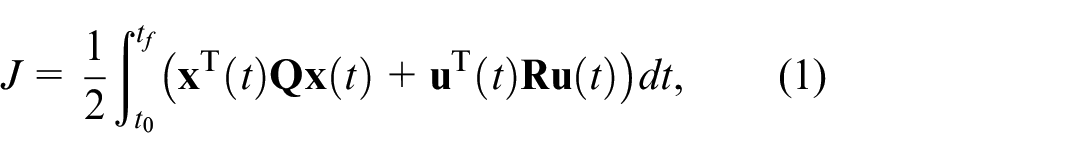
The optimal control theory is aimed to minimize the performance index function constrained by a specific state path for dynamic system. In order to take positive and negative deviations from the optimal control signal into account, one may consider the absolute or quadratic forms.24,33 However, it would be mathematically straightforward to deal with the quadratic formulation. So, it is aimed to minimize the following quadratic form of the cost function
subjected to the state equation

and initial/terminate conditions

where the state variables are
and
Solution strategy
In order to solve the optimal control problem of finding
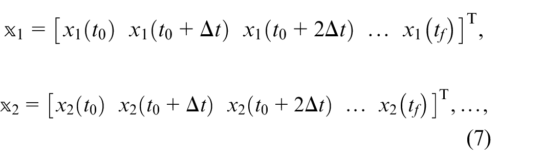
First, the time domain is discretized by n equally-space points

So, the state and control variables will have the following discretized forms
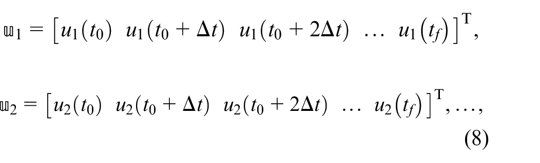
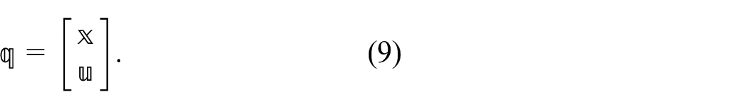
and one has the total unknown parameters in the form of the augmented vector of both states and control efforts of order
Now, the numerical differentiation and integration operators can be introduced. According to the time discretization, the finite difference method could be an appropriate candidate to evaluate derivatives in the state equation. If, we consider the discretized form of a typical function
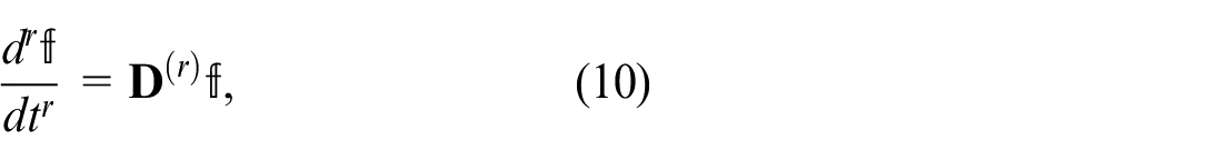
where,
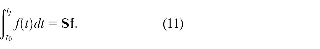
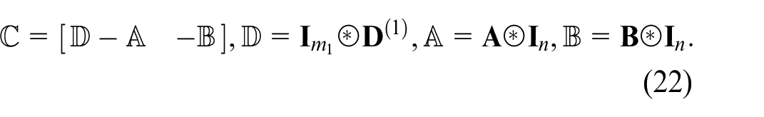
In order to calculate the integral value at the same points of time discretization, the integral operator must be proportional to the differential one.
28
The idea of variational differential quadrature approach is used herein to develop the variational finite difference solution methodology and tackle the optimal control problems. Thus, the corresponding approach can be adopted here to obtain the integral operator vector
Therefore, using the discretization of the quadratic form of the integrand, the algebraic form of equation (1) is accordingly obtained as
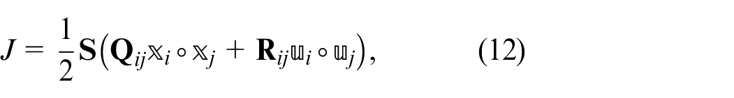
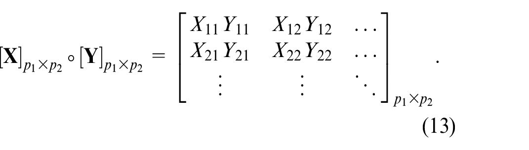
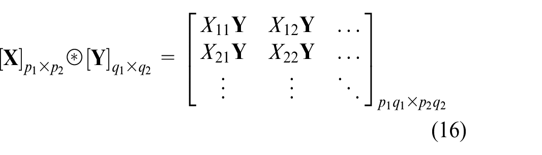
where i and j stand for the vector indexes and ° shows the Hadamard product with the following definition
from the lemma
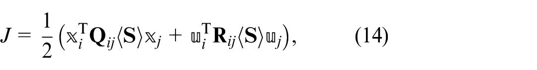
which can also be given in the following total matrix representation
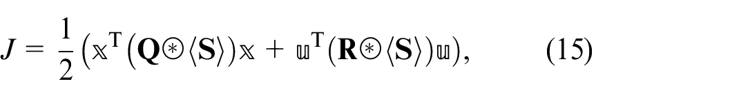
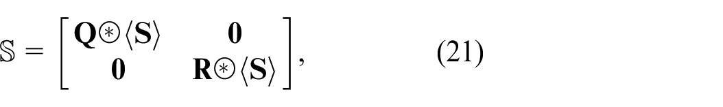
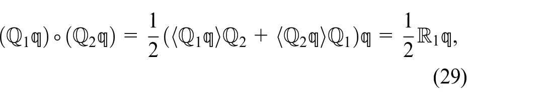
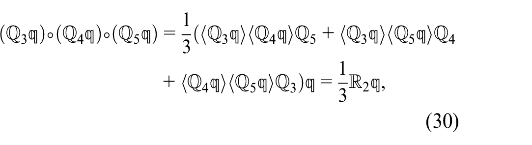
where
Also, discretization of equation (2) leads to
where
Therefore, the cost function, state equation, and the corresponding boundary conditions in equation (3) are, respectively, represented in the following forms


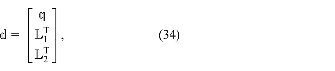
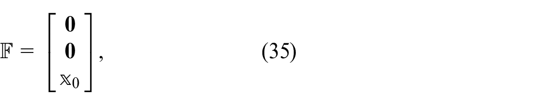
where
and
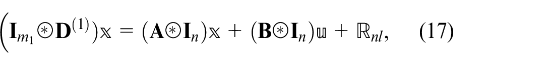
As a result of the developed VFD formulation and instead of the primary integro-differential-algebraic equations in equations (1)–(3), the design of the optimal control problem is now observed as that a system of
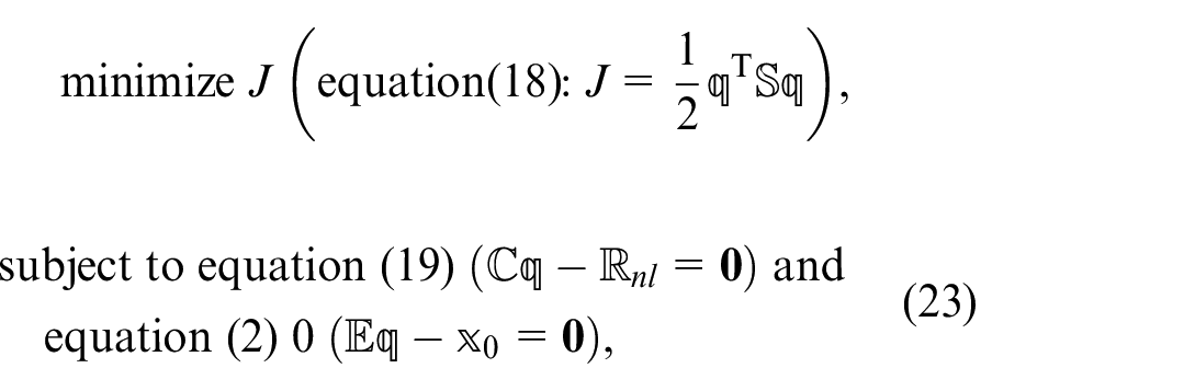
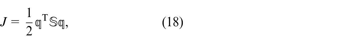
and the Lagrange function is given by
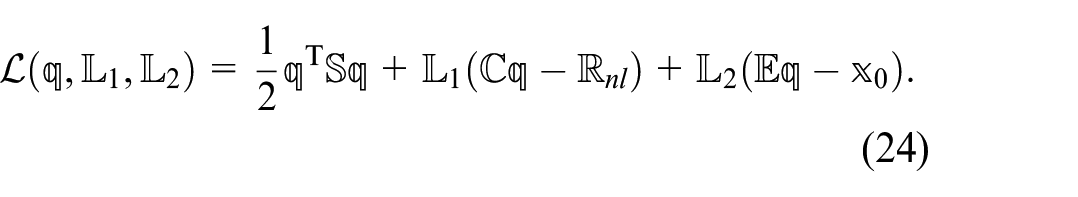
where
Setting the gradient of the Lagrange function equal to zero, the governing equations would be determined (i.e.
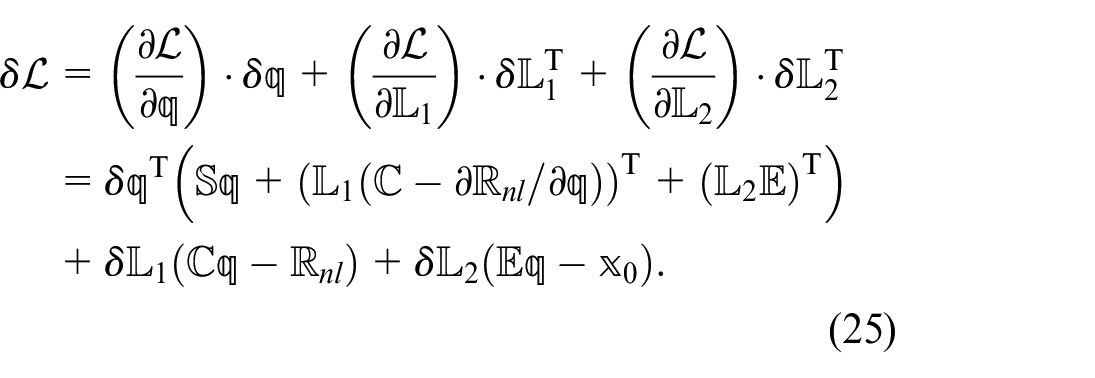
The necessary condition of vanishing the first variation of the Lagrange function, that is,


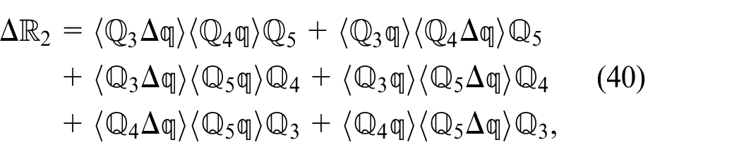
Such obtained nonlinear set of equations can now be solved in a straightforward manner by utilizing the iterative solution procedure of Newton-based methods. Here, an explicit form of nonlinearity, if any, is considered to complete the formulation. In this way, it is assumed that the nonlinear vector is consisted of second- and third-order terms so that the quadratic and triadic nonlinearities are, respectively, given by
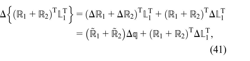
where
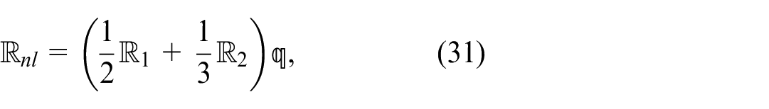
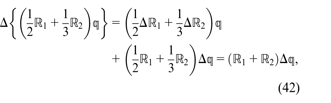
which results that (see Appendix C)
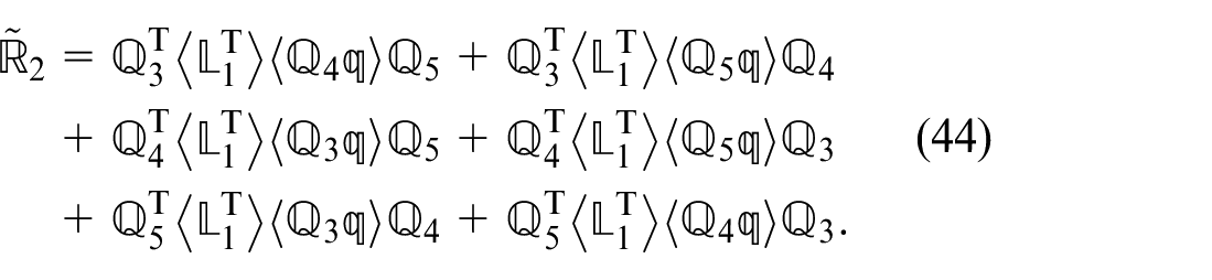
Thus, from equations (26)–(28) to equations (31)–(32), the final equation reads

where
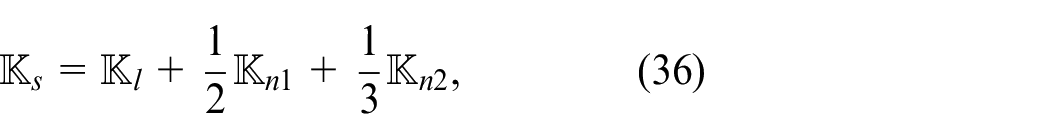
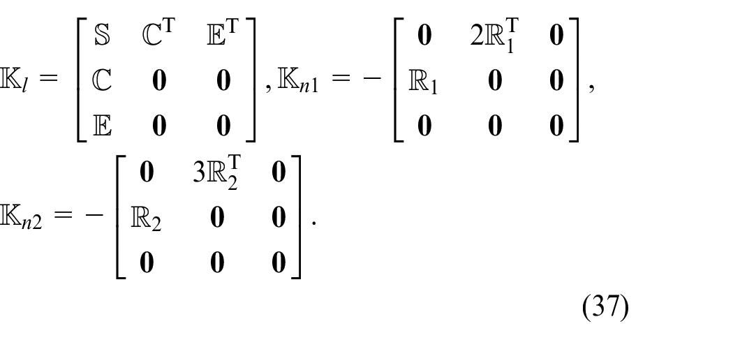
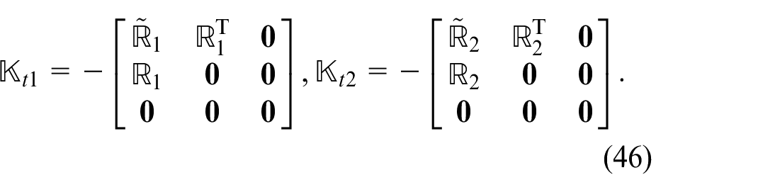
and the stiffness matrix
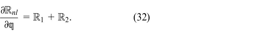
In addition of the above-mentioned formulation, the Jacobi of nonlinear algebraic equations is required in Newton approach. Deriving the incremental form of equation (25), one has
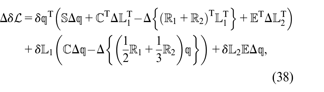
considering

and the lemma
where

So, the tangent stiffness matrix is achieved as follows

and as a result, the solution of equation (33) is obtained iteratively as
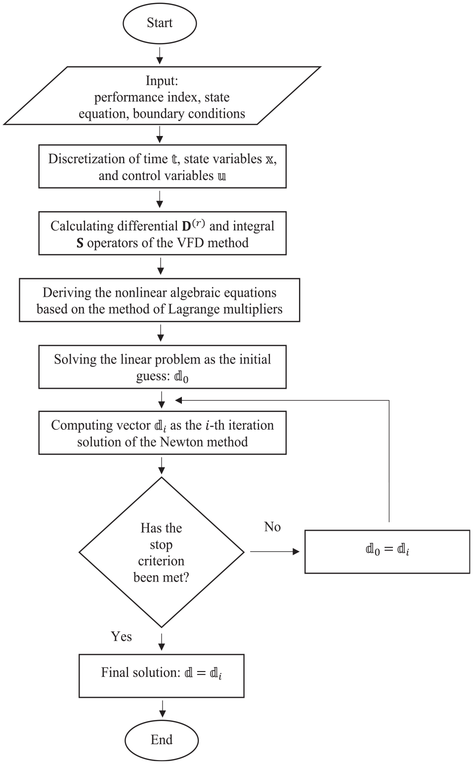
Flowchart of the solution strategy.
Selected case studies
In this section, the accuracy and efficiency of the proposed VFD method for the analyzing of both linear and nonlinear optimal control problems are examined through several case studies. In different examples, the convergence of results based on the VFD method is investigated. Also, to examine the validity of present study, the obtained results are compared with those of available in open literature, that is, with the paper of Jaddu
6
and Mohammadi et al.
24
It should be noted that for
Linear time-invariant system (manned spacecraft)
As the first case study, consider the following cost function, state equations and conditions24,33
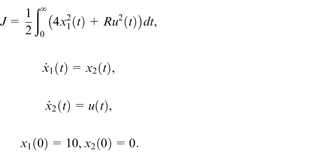
Comparing with the represented matrix formulation, one has
It is assumed that
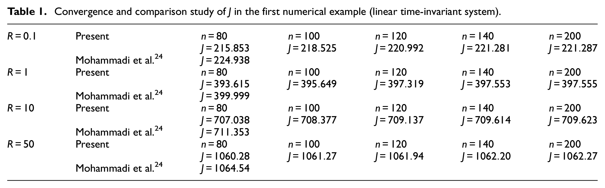
The produced numerical results are given in Table 1 and Figure 2. Considering different number of discretization points for the finite difference method, the values of performance index are reported in Table 1. Accordingly, the appropriate convergence behavior and validity of the proposed solution approach can be clearly observed. Corresponding to different values of R, time responses of the state variables are displayed in Figure 2. It is revealed that the same results of references are obtained via the VFD method. The average run time of this case is about 0.09 s.
Convergence and comparison study of J in the first numerical example (linear time-invariant system).
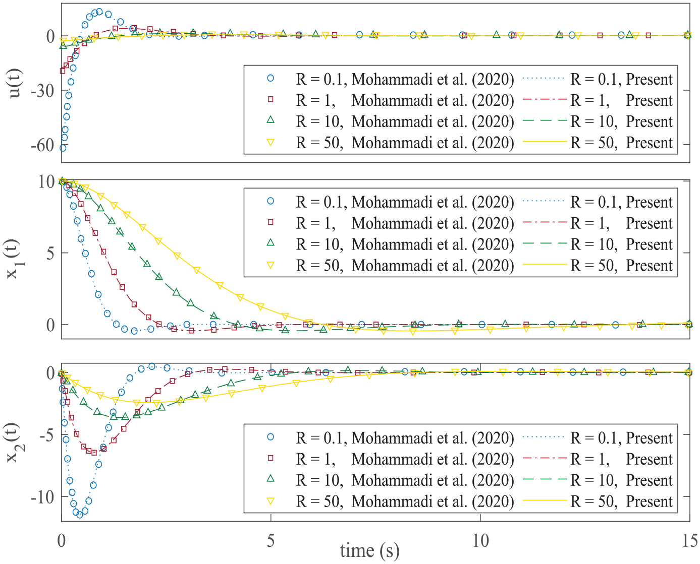
Transient responses of the first case study (linear time-invariant system).
Linear time-variant system
The second numerical example is dedicated to the analysis of a time-variant system. The problem is identified with24,34
So, the parameters are
According to what mentioned earlier, the discretized form of matrix
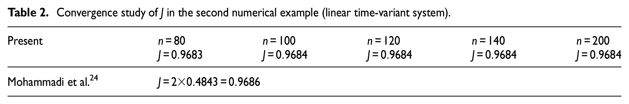
Table 2 shows the rich convergence of the proposed solution method to solve the time-variant problem. In Figure 3, the variation of the parameters x and u are plotted versus time. Also, a verification study is made with the reported results of literature. The time of analysis is 0.04 s which is far less than the previous attempts such as the ones based on genetic algorithm24,35 or MPC.25–27
Convergence study of J in the second numerical example (linear time-variant system).
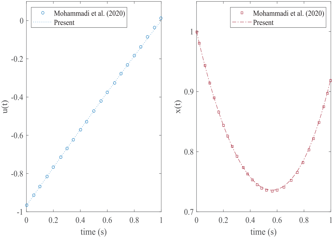
Transient responses of the second case study (linear time-variant system).
Nonlinear system (Van der Pol problem)
In this case, the following optimal control problem with nonlinear state equations is considered24,35
So, one has
The discretized form of
From boundary conditions,
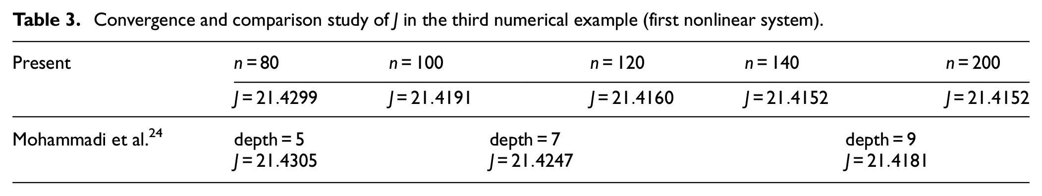
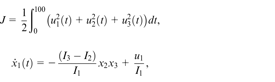
Now, like the previous case studies, the convergence behavior and transient responses of the system are studied. From Table 3, the converged performance index can be compared with different values reported in Mohammadi et al.
24
It is observed that there is a very good agreement with the more precise case (
Convergence and comparison study of J in the third numerical example (first nonlinear system).
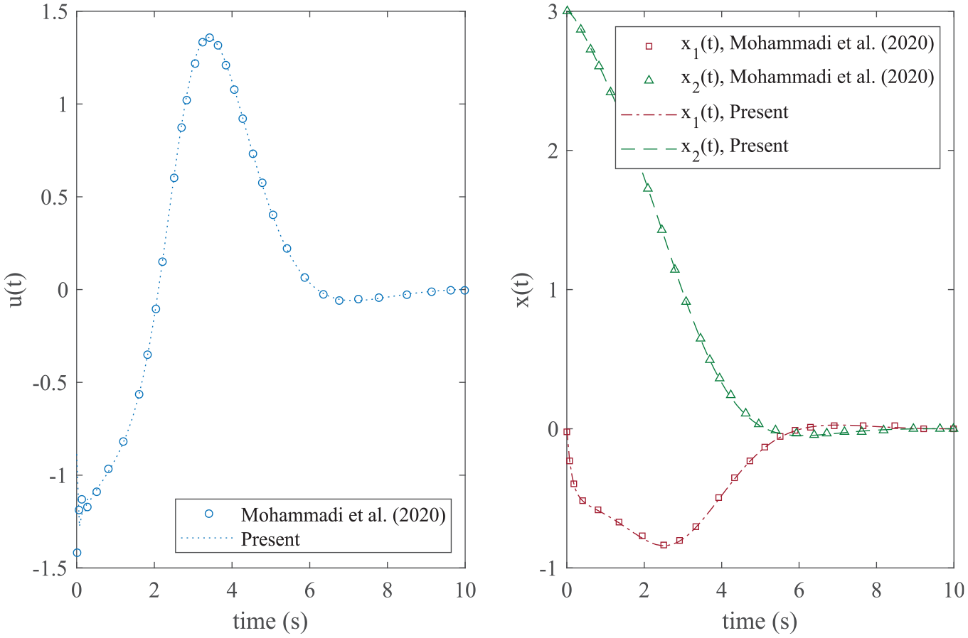
Transient responses of the third case study (first nonlinear system).
Nonlinear system (Rigid asymmetric spacecraft)
As the last example, the VFD method is used to solve the following nonlinear system 6
where
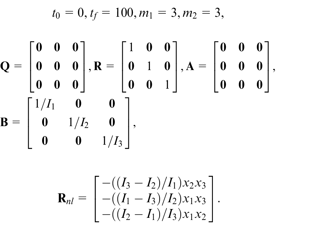
Also,
and
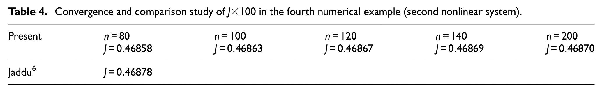
The numerical results of this example involving convergence and comparative studies as well as time responses can be found in Table 4 and Figure 5. Comparing the performance index and transient solutions for the six state parameters, it is observed that the obtained results are in excellent agreement with Jaddu. 6 Also, the time of nonlinear analysis of the optimal control problem is 0.67 s for two iterations. Like the previous nonlinear case study, it is seen that the present solution methodology is reliable and efficient. Comparing with the computational demand of the available nonlinear programming algorithms, the executed run time of nonlinear case studies could be promising for future attempts in the area of optimal control theory.
Convergence and comparison study of
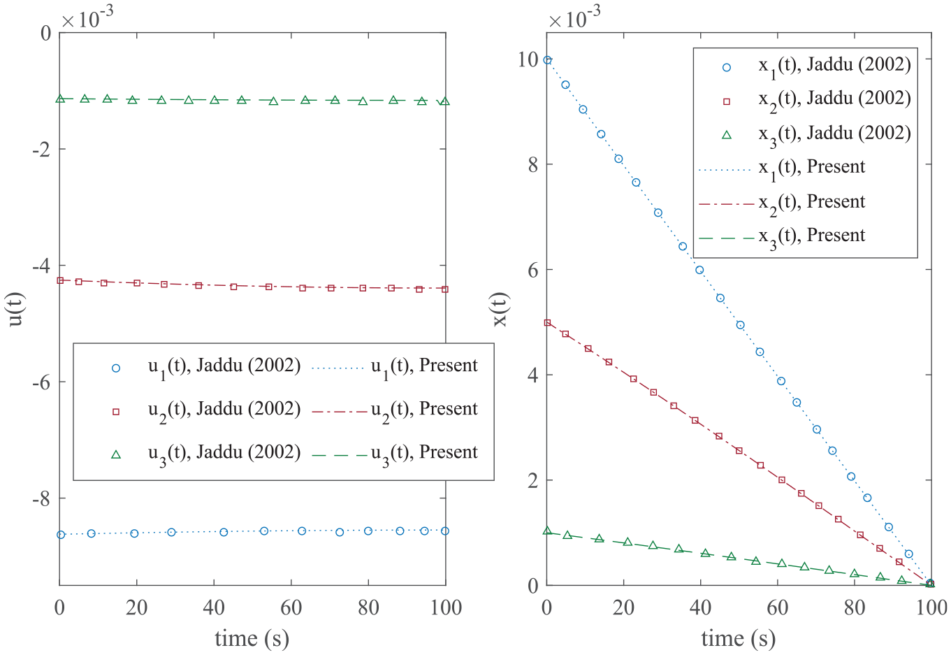
Transient responses of the fourth case study (second nonlinear system).
Computational efficiency
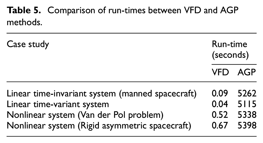
The straightforward mathematical formulation as well as the accuracy of VFD method has been shown so far. Here, some comparisons are made to show the computational efficiency of the variational finite difference approach in context of the optimal control theory. In this regard, the numerical case studies are solved via the archived-based genetic programming as the recent attempt in this research area. 24 To be ensure of the accuracy of the run-times reported for the proposed VFD method, several runs were performed and the average values are considered. In addition, tabulated in Table 5 are the executed run-times obtained from AGP solution of the single-objective optimal control problems with 200 generations. Results are quite promising and clearly reveal the efficiency of the suggested solution strategy.
Comparison of run-times between VFD and AGP methods.
Concluding remarks
A novel solution was proposed in the context of nonlinear quadratic optimal control problems using variational time discretized finite difference approach inspired from the variational differential quadrature method. Also, with the aim of straightforward implementation of solution strategy, a matrix-vector formulation was conveniently developed for the performance index, state equations, and boundary conditions usually represented in optimal control problems. The resulted algebraic equations of the minimization problem were then solved with the help of the Lagrange multiplier method. Due to utilizing consistent integral/differential operators and the analytical tangent stiffness matrix rather than the numerical Jacobian, the developed methodology is robust and more efficient in comparison with the available solutions in literature. Such a claim was supported with successfully analyzing different case studies including the linear time-invariant, linear time-variant and nonlinear systems. The significant efficiency of the developed VFD method could be find from the fact that the run time of analysis was less than 1 s even in case of nonlinear optimal control problems. In future communications, the proposed approach will be extended for the case of multi-dimensional nonlinear optimal control problems.
Footnotes
Appendix A
To evaluate derivatives of function
For instance
For instance
So, one can write
Appendix B
According to Shojaei and Ansari (28), the Taylor series representation of a function is used to evaluate the integral operator at the same points on which the differentiation is calculated. In a neighborhood of a typical point
Since
Considering the whole intervals of discretization scheme, it results that
where,
Appendix C
The variation of discretized nonlinear state vector (equation (31)) is calculated as
Considering equation (29), equation (30) and the lemma
and thus, it is shown that
Declaration of conflicting interests
The author(s) declared no potential conflicts of interest with respect to the research, authorship, and/or publication of this article.
Funding
The author(s) received no financial support for the research, authorship, and/or publication of this article.
Data availability
The datasets generated and analyzed during the current study are not publicly available due the data also forms part of an ongoing study but are available from the corresponding authors on reasonable request.