The convergence of a numerical method for total variation flow

Abstract

We present a convergence analysis for a finite difference scheme for the time dependent partial different equation called gradient flow associated with the Rudin-Osher-Fetami model. We devise an iterative algorithm to compute the solution of the finite difference scheme and prove the convergence of the iterative algorithm. Finally computational experiments are shown to demonstrate the convergence of the finite difference scheme.

Introduction

The well-known ROF model may be approximated in the following way

$$\underset{u\in \text{BV}(\Omega )}{\min }{\displaystyle {\int }_{\Omega }\sqrt{\mathrm{ϵ}+|\nabla u{|}^2}}\mathrm{d}x+\frac{1}{2\lambda }{\displaystyle {\int }_{\Omega }|}u-f{|}^2\mathrm{d}x$$

(1)

As $\mathrm{ϵ}>0$ , the above minimizing functional is differentiable. Thus, the Euler-Lagrange equation associated with the above minimization is

$$\text{div}\left(\frac{\nabla u}{\sqrt{\mathrm{ϵ}+|\nabla u{|}^2}}\right)-\frac{1}{\lambda }(u-f)=0$$

(2)

Solution of this partial differential equation can be further approximated. Let us consider the time evolution version of the PDE:

$$\{\begin{array}{l}\frac{d}{dt}u=\text{ div }\left(\frac{\nabla u}{\sqrt{\mathrm{ϵ}+|\nabla u{|}^2}}\right)-\frac{1}{\lambda }(u-f),\in {\Omega }_T,\hfill \\ \frac{\partial }{\partial \mathbf{n}}u=0,\text{on }\partial {\Omega }_T,\hfill \\ u(·,0)=u_0(·)\Omega ,\hfill \end{array}$$

(3)

where ${\Omega }_T=[0,T)\times \Omega ,\frac{\partial }{\partial \mathbf{n}}$ is the outward normal derivative operator. It is called the gradient flow of (1). When ϵ = 0, it is called TV flow. When using ROF for the purpose of denoising image, f is a given noised image, and u is the denoised image. Similar partial differential equations also appear in geometry analysis. See references, e.g., Lichnewsky and Temam,¹ Gerhardt,² Andreu et al.,^3–5 and the references therein. The existence, uniqueness, stability of the weak solutions to these time dependent PDE were studied in the literature mentioned above. Numerical solution of the PDE (3) using finite elements has been discussed in Feng and Prohl ⁶ and Feng et al.⁷ In particular, the researchers showed that the finite element solution exists, is unique, is convergent to the weak solution of the PDE (3), the rate of convergence under some sufficient conditions, and the computation is stable. Numerical solution to the weak solution using bivariate spline method and its convergence was studied in Hong et al. ⁸ A fixed point iterative algorithm for the associated system of nonlinear equations was discussed in Vogel and Oman ⁹ and its convergence was studied in Dobson and Vogel. ¹⁰ An algorithm based on the split Bregman iterations was discussed in Li et al. ¹¹ In Khan et al. ¹² gave an a mesh-free algorithm to solve the ROF model. Although the finite difference solution of the time dependent PDE (3) has been the method of choice for image denoising (e.g. See Vese and Osher ¹³ ), no convergence of the finite difference solution to the weak solution of the PDE has been established in the literature so far to the best of the authorsal methods for p-harmo Feng and authors' knowledge Lai.

The purpose of this paper is to establish the convergence of the discrete solution obtained from a finite difference scheme for (3) to the weak solution. See our Theorem 3.4. Then we discuss how to numerically solve the time dependent PDE (3) by using our finite difference scheme. As the finite difference scheme is a system of nonlinear equations, we shall derive an iterative algorithm and show that the iterative solutions are convergent.

For convenience, let $\Omega =[0,1]\times [0,1]$ . We let N > 0 be a positive integer and divide y solve the time dependent x_i = ih and y_j = jh for $0\le i,j\le N-1$ where $h=1/N$ . For any f(x, y) defined on ve let $f_{i,j}^h=f(x_i,y_j)$ . We shall use two different divided differences ${\nabla }^{+}$ and ${\nabla }^{-}$ to approximate the gradient operator. That is,

$${\nabla }^{+}{f}_{i,j}^h=\left(\frac{f_{i+1,j}^h-f_{i,j}^h}{h},\frac{f_{i,j+1}^h-f_{i,j}^h}{h}\right)$$

and

$${\nabla }^{-}{f}_{i,j}^h=\left(\frac{f_{i,j}^h-f_{i-1,j}^h}{h},\frac{f_{i,j}^h-f_{i,j-1}^h}{h}\right)$$

for all $0\le i,j\le N-1$ with $f_{-1,j}^h=f_{0,j}^h,f_{N,j}^h=f_{N-1,j}^h$ for all j and $f_{i,-1}^h=f_{i,0}^h,f_{i,N}^h=f_{i,N-1}^h$ for all i. Furthermore, we define discrete divergence operators ${\text{div}}^{+}$ and ${\text{div}}^{-}$ to approximate the continuous divergence operator, i.e., suppose the grid size is h > 0,

$$\begin{array}{l}({\text{div}}^{+}p)i,j=\{\begin{array}{l}{p}_{i,j}^1/h,i=0,\hfill \\ (p_{i,j}^1-p_{i-1,j}^1)/h,0<i<N-1,\hfill \\ -p_{i-2,j}^1/h,i=N-1\hfill \end{array}\\ +\{\begin{array}{l}{p}_{i,0}^2/h,j=0,\hfill \\ (p_{i,j}^2-p_{i,j-1}^2)/h,0<j<N-1,\hfill \\ -p_{i,j-2}^2/h,j=N-1,\hfill \end{array}\end{array}$$

for all $0\le i,j\le N-1$ and similarly for ${\text{div}}^{-}$ . By their definitions, we have for every $p\in {ℝ}^{N\times N}\times {ℝ}^{N\times N}$ and $u\in {ℝ}^{N\times N}$

$$〈-{\text{div}}^{+}p,u〉=〈p,{\nabla }^{+}u〉,〈-{\text{div}}^{-}p,u〉=〈p,{\nabla }^{-}u〉$$

With these notations, we are able to define a finite difference scheme for numerical solution of the time dependent PDE (3).

$$\{\begin{array}{l}\frac{d}{dt}{u}_{i,j}=\frac{1}{2}{\text{ div}}^{+}\left(\frac{{\nabla }^{+}{u}_{i,j}}{\sqrt{\mathrm{ϵ}+|{\nabla }^{+}{u}_{i,j}{|}^2}}\right)\hspace{0.17em}\hfill \\ +\frac{1}{2}{\text{ div}}^{-}\left(\frac{{\nabla }^{-}{u}_{i,j}}{\sqrt{\mathrm{ϵ}+|{\nabla }^{-}{u}_{i,j}{|}^2}}\right)-\frac{1}{\lambda }(u_{i,j}-f_{i,j}^h)\hspace{0.17em}\hfill \\ 0\le i,j\le N-1,t\in [0,T],\hspace{0.17em}\hfill \\ \frac{\partial }{\partial \mathbf{n}}{u}_{i,j}=0\hspace{0.17em}\hfill \\ i=0,N,0\le j\le N-1;\hspace{0.17em}\hfill \\ j=0,N,0\le i\le N-1\hspace{0.17em}\hfill \\ u(x_i,y_j,0)=u_0(x_i,y_j),\hspace{0.17em}\hfill \\ 0\le i,j\le N-1\hspace{0.17em}\hfill \end{array}$$

(4)

Next we discretize the time domain $[0,T]$ by equally-spaced points $t_k=k\Delta t,\Delta t=T/M$ . We approximate the $\frac{d}{dt}{u}_{i,j}$ by $(u_{i,j}^k-u_{i,j}^{k-1})/\Delta t$ to have the fully discrete version of finite difference scheme:

$$\{\begin{array}{l}\frac{1}{\Delta }t(u_{i,j}^k-u_{i,j}^{k-1})=\frac{1}{2}{\text{ div}}^{+}\left(\frac{{\nabla }^{+}{u}_{i,j}^k}{\sqrt{\mathrm{ϵ}+|{\nabla }^{+}{u}_{i,j}^k{|}^2}}\right)\hspace{0.17em}\hfill \\ +\frac{1}{2}{\text{ div}}^{-}\left(\frac{{\nabla }^{-}{u}_{i,j}^k}{\sqrt{\mathrm{ϵ}+|{\nabla }^{-}{u}_{i,j}^k{|}^2}}\right)-\frac{1}{\lambda }(u_{i,j}^k-f_{i,j}^h),\hspace{0.17em}\hfill \\ 0\le i,j\le N-1,1\le k\le M\hspace{0.17em}\hfill \\ \frac{\partial }{\partial \mathbf{n}}{u}_{i,j}^k=0,\hspace{0.17em}\hfill \\ i=0,N,0\le j\le N-1;\hspace{0.17em}\hfill \\ j=0,N,0\le i\le N-1,\hspace{0.17em}\hfill \\ 0\le k\le M\hspace{0.17em}\hfill \\ u(x_i,y_j,0)=u_0(x_i,y_j),0\le i,j\le N-1\hspace{0.17em}\hfill \end{array}$$

(5)

Remark 1.1. In our numerical scheme, the discrete variation for any array $u^k:=\{u_{ij}^k,0\le i,j\le N\}$ is in fact defined by

$$|u^k{|}_{\text{DBV}}=\frac{1}{2}{\displaystyle \sum _{i,j}\sqrt{\mathrm{ϵ}+|{\nabla }^{+}{u}_{i,j}^k{|}^2}}+\frac{1}{2}{\displaystyle \sum _{i,j}\sqrt{\mathrm{ϵ}+|{\nabla }^{-}{u}_{i,j}^k{|}^2}}$$

This way of defining discrete variation makes it possible to connect discrete and continuous variations by the observation that $|U{|}_{\text{BV}}=|u^k{|}_{\text{DBV}}$ where U is a piecewise linear function obtained by interpolating u^k over grids on iecewise linear function obtained by interpolating ct discrete and continuous variations by the observation that rence scheme is a system of nonli

$$\arg \min E_k(v)$$

for each step k where

$$\begin{array}{l}{E}_k(v)=\frac{1}{2}{\displaystyle \sum _{i,j}\sqrt{\mathrm{ϵ}+|{\nabla }^{+}{v}_{i,j}{|}^2}}{h}^2+\frac{1}{2}{\displaystyle \sum _{i,j}\sqrt{\mathrm{ϵ}+|{\nabla }^{-}{v}_{i,j}{|}^2}}{h}^2\\ +\frac{1}{2\lambda }{\displaystyle \sum _{i,j}{(v_{i,j}-f_{i,j}^h)}^2}{h}^2+\frac{1}{2\Delta t}{\displaystyle \sum _{i,j}{(v_{i,j}-u_{i,j}^{k-1})}^2}{h}^2\end{array}$$

for all arrays $\left\{v_{i,j}\right\},0\le i,j\le N-1$ .

We shall first show that the above scheme has a uniqueness solution. Then we show the solution in (5) converges to the weak solution of time dependent PDE (3). These will be done in the next 2 sections. Next we shall explain how to numerically solve this system of nonlinear equations in the Section 4. We report our computational results in the Section 5. Finally we give a few remarks the last section.

Preliminary results

We introduce a weak formulation of PDE (3) that is suggested by Feng and Prohl.⁶

Definition 2.1. We say that $u\in L^1([0,T],\text{BV}(\Omega ))$ is a weak solution of (3) if u satisfies the initial value and boundary conditions in (3) and for any $w\in L^1([0,T],W^{1,1}(\Omega ))$ with $\frac{\partial }{\partial \mathbf{n}}w(x,t)=0$ for all $(t,x)\in [0,T)\times \partial \Omega$ ,

$$\begin{array}{l}{\displaystyle {\int }_0^s{\displaystyle {\int }_{\Omega }\frac{d}{dt}}}u\mathit{w}\mathrm{d}x\mathrm{d}t+{\displaystyle {\int }_0^s{\displaystyle {\int }_{\Omega }\frac{\nabla u·\nabla w}{\sqrt{\mathrm{ϵ}+|\nabla u{|}^2}}}}+\\ \frac{1}{\lambda }{\displaystyle {\int }_0^s{\displaystyle {\int }_{\Omega }(u-f)}}w\mathrm{d}x\mathrm{d}t=0\end{array}$$

(6)

for any $s\in (0,T]$ .

It is known (cf. Feng and Prohl⁶) there exists a unique weak solution $U^{*}$ satisfying the above weak formulation. $U^{*}$ is in fact in $L^{\infty }((0,T],\text{BV}(\Omega ))$ if $u^0\in \text{BV}(\Omega )$ and $f\in L^2(\Omega )$ . Following the ideas in Lichnewsky and Temam,¹ the researchers in Feng and Prohl⁶ further showed the weak solution can be characterized by the following inequality.

Theorem 2.1. Let u be a weak solution as in Definition 2.1. Then u satisfies the following inequality: for any $s\in (0,T]$ ,

$$\begin{array}{l}{\displaystyle {\int }_0^s{\displaystyle {\int }_{\Omega }\frac{d}{dt}}}v(v-u)\mathrm{d}x\mathrm{d}t+{\displaystyle {\int }_0^s(J(}v)-J(u))\mathrm{d}t\ge \\ \frac{1}{2}\left[{\displaystyle {\int }_{\Omega }(v(}x,s)-u(x,s){)}^2\mathrm{d}x-{\displaystyle {\int }_{\Omega }(v(}x,0)-u_0(x,0){)}^2\mathrm{d}x\right]\end{array}$$

(7)

for all $v\in L^1([0,T],W^{1,1}(\Omega ))$ with $\frac{\partial }{\partial \mathbf{n}}v(x,t)=0$ for all $(t,x)\in [0,T)\times \partial \Omega$ , where

$$\begin{array}{l}J(u)={\displaystyle {\int }_{\Omega }\sqrt{\mathrm{ϵ}+|\nabla u(x,t){|}^2}}\mathrm{d}x+\\ \frac{1}{2\lambda }{\displaystyle {\int }_{\Omega }|}f(x,t)-u(u,t){|}^2\mathrm{d}x\end{array}$$

(8)

On the other hand, if a function $u\in L^1((0,T],\text{BV}(\Omega ))$ satisfies the above inequality (7), then u is a weak solution.

Regarding to the solution of finite difference scheme (5), we prove some basic properties in this section. To this end, we assume that the initial data for our numerical scheme $\{f_{i,j}^h,0\le i,j\le N-1\}$ is a discretization of the initial data for PDE (3). Specifically assuming the region $\Omega =[0,1]\times [0,1]$ is partitioned evenly into N by N grids with a grid size of $h=1/N$ , we suppose

$$f_{i,j}^h=\frac{1}{h^2}{\displaystyle {\int }_{ih}^{(i+1)h}{\displaystyle {\int }_{jh}^{(j+1)h}f}}(x)\mathrm{d}x,0\le i,j\le N-1$$

i.e., the pixel value on each grid with index (i, j) is $f_{i,j}^h$ . In the next section we sometimes denote by $P_{N}f$ a related piecewise constant function defined on Ω for which

$$(P_{N}f)(x)=f_{i,j}^h,x\in [ih,(i+1)h]\times [jh,(j+1)h].$$

(9)

Let us start with the following existence and uniqueness theorem.

Theorem 2.2. Fix N > 0 and M > 0. There exists a unique array $u_{i,j}^k,0\le i,j\le N-1,0\le k\le M$ satisfying the above system of nonlinear equations.

Proof. We define a variation functional that is a discretized version of (8)

$$\begin{array}{l}{J}^h(v)=\frac{1}{2}{\displaystyle \sum _{i,j}\sqrt{\mathrm{ϵ}+|{\nabla }^{+}{v}_{i,j}{|}^2}}{h}^2+\\ \frac{1}{2}{\displaystyle \sum _{i,j}\sqrt{\mathrm{ϵ}+|{\nabla }^{-}{v}_{i,j}{|}^2}}{h}^2+\frac{1}{2\lambda }{\displaystyle \sum _{i,j}{(v_{i,j}-f_{i,j}^h)}^2}{h}^2\end{array}$$

(10)

and the discrete energy functional

$$E^h(v)=J^h(v)+\frac{1}{2\Delta t}{\displaystyle \sum _{i,j}{(v_{i,j}-u_{i,j}^{k-1})}^2}{h}^2$$

(11)

for all arrays $v_{i,j},0\le i,j\le N-1$ .

The Euler-Lagrange equation for the following minimization problem

$$\underset{v}{\min }{E}^h(v)$$

(12)

is

$$\begin{array}{l}\frac{u_{i,j}^k-u_{i,j}^{k-1}}{\Delta }t-\frac{1}{2}{\text{ div}}^{+}\left(\frac{{\nabla }^{+}{u}_{i,j}^k}{\sqrt{\mathrm{ϵ}+|{\nabla }^{+}{u}_{i,j}^k{|}^2}}\right)\\ -\frac{1}{2}{\text{ div}}^{-}\left(\frac{{\nabla }^{-}{u}_{i,j}^k}{\sqrt{\mathrm{ϵ}+|{\nabla }^{-}{u}_{i,j}^k{|}^2}}\right)+\frac{1}{\lambda }(u_{i,j}^k-f_{i,j}^h)=0,\\ 0\le i,j\le N-1,1\le k\le M\end{array}$$

(13)

The existence and uniqueness of $u_{i,j}^k$ follows from the strict convexity of the functional J^h and E^h.

The following property is a characterization of the discrete solution of (5).

Lemma 2.1. Suppose that array $\{u_{i,j}^k,0\le i,j\le N-1,0\le k\le M\}$ is a solution of the finite difference scheme (5). Then $u_{i,j}^k$ satisfies the following inequality

$$\begin{array}{l}{\displaystyle \sum _{i,j}\frac{u_{i,j}^k-u_{i,j}^{k-1}}{\Delta }}t(v_{i,j}-u_{i,j}^k)\\ +\frac{1}{2}\left({\displaystyle \sum _{i,j}\sqrt{\mathrm{ϵ}+|{\nabla }^{+}{v}_{i,j}{|}^2}}-{\displaystyle \sum _{i,j}\sqrt{\mathrm{ϵ}+|{\nabla }^{+}{u}_{i,j}^k{|}^2}}\right)\\ +\frac{1}{2}\left({\displaystyle \sum _{i,j}\sqrt{\mathrm{ϵ}+|{\nabla }^{-}{v}_{i,j}{|}^2}}-{\displaystyle \sum _{i,j}\sqrt{\mathrm{ϵ}+|{\nabla }^{-}{u}_{i,j}^k{|}^2}}\right)\\ +\frac{1}{2\lambda }{\displaystyle \sum _{i,j}{(v_{i,j}-f_{i,j}^h)}^2}-\frac{1}{2\lambda }{\displaystyle \sum _{i,j}{(u_{i,j}^k-f_{i,j}^h)}^2}\\ \ge 0\end{array}$$

(14)

for all arrays $v_{i,j}$ that satisfies the Neumann boundary condition. On the other hand, if an array $\{u_{i,j}^k,0\le i,j\le N-1,0\le k\le M\}$ satisfies the above inequality for all $v_{i,j}$ satisfying the discrete Neumann boundary condition in (5), then array $\{u_{i,j}^k,0\le i,j\le N-1\}$ is a solution of (5).

Proof. From the Euler-Lagrange equation (13),

$$\begin{array}{l}\frac{u_{i,j}^{k-1}-u_{i,j}^k}{\Delta }t=\partial J^h(u_{i,j}^k)\\ =-\frac{1}{2}{\text{ div}}^{+}\left(\frac{{\nabla }^{+}{u}_{i,j}^k}{\sqrt{\mathrm{ϵ}+|{\nabla }^{+}{u}_{i,j}^k{|}^2}}\right)\\ -\frac{1}{2}{\text{ div}}^{-}\left(\frac{{\nabla }^{-}{u}_{i,j}^k}{\sqrt{\mathrm{ϵ}+|{\nabla }^{-}{u}_{i,j}^k{|}^2}}\right)\\ +\frac{1}{\lambda }(u_{i,j}^k-f_{i,j}^h)\end{array}$$

The result follows from the definition of subgradient $\partial J^h(u^k)$ .

The following result shows that the computation of finite difference scheme (5) is stable. For the simplicity of the notations, we define the discrete L² norms in analogue of standard L² norms. Assuming $\left\{u_{i,j}\right\}$ is an array, we define

$$\left|\right|u\left|\right|:={\left\{{\displaystyle \sum _{i,j}{(u_{i,j})}^2}{h}^2\right\}}^{1/2}$$

Theorem 2.3. Let $\{u_f^k,0\le k\le M\}$ be the solution of the system of nonlinear equations (5) associated with f^h with initial value $u_f^0$ . Similarly, let $\{u_g^k,0\le k\le M\}$ be the corresponding solution of (5) associated with g^h with initial value $u_g^0$ . Then

$$\left|\right|u_f^k-u_g^k\left|\right|\le \max \left\{\right||u_f^0-u_g^0||,||f^h-g^h|\left|\right\},1\le k\le M$$

(15)

Proof. We prove by induction. It is obvious true for k = 0. Assume the inequality holds for k . Assume the inequa L² terms in (12). We have $u_f^k$ is the minimizer of the following problem.

$$\begin{array}{l}\underset{v}{\min }\frac{h^2}{2}{\displaystyle \sum _{i,j}\sqrt{\mathrm{ϵ}+|{\nabla }^{+}{v}_{i,j}{|}^2}}+\frac{h^2}{2}{\displaystyle \sum _{i,j}\sqrt{\mathrm{ϵ}+|{\nabla }^{-}{v}_{i,j}{|}^2}}\\ +({\mu }_1+{\mu }_2){\Vert v-\left(k_1{f}^h+k_2{u}_f^{k-1}\right)\Vert }^2\end{array}$$

(16)

where ${\mu }_1=1/(2\lambda ),{\mu }_2=1/2\Delta t$ , and $k_1={\mu }_1/({\mu }_1+{\mu }_2),k_2={\mu }_2/({\mu }_1+{\mu }_2)$ . By standard stability property of the minimization problem (16) (cf. Lucier and Wang ¹⁴ )

$$\begin{array}{l}\Vert u_f^k-u_g^k\Vert \le \Vert \left(k_1{f}^h+k_2{u}_f^{k-1}\right)-\left(k_1{g}^h+k_2{u}_g^{k-1}\right)\Vert \\ \le k_1\left|\right|f^h-g^h\left|\right|+k_2\Vert u_f^{k-1}-u_g^{k-1}\Vert \\ \le \max \left\{\left|\right|f^h-g^h\left|\right|,\Vert u_f^{k-1}-u_g^{k-1}\Vert \right\}\\ \le \max \left\{\left|\right|f^h-g^h\left|\right|,\Vert u_f^0-u_g^0\Vert \right\}\end{array}$$

Remark 2.2. As a direct deduction, if $g^h=u_g^0=0$ , the solution $u_g^k$ is also zero for all k, then

$$\left|\right|u_f^k\left|\right|\le \max \left\{\right|\left|u_f^0\right||,|\left|f^h\right|\left|\right\},1\le k\le M$$

(17)

Main result and its proof

In this section, we shall show that the solution of the finite difference scheme (5) converges to the solution of the gradient flow (3). We suppose that the array $\{u_{i,j}^k,0\le i,j\le N-1,0\le k\le M\}$ is the solution of (5).

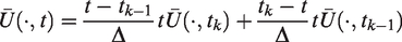
We first define a mapping of the array $\{u_{i,j}^k,0\le i,j\le N-1,0\le k\le M\}$ in the form of a piecewise linear interpolant of $u_{i,j}^k$ .

Let t _N be the following type of triangulation of $\Omega =[0,1]\times [0,1]$ with vertices $((i+1/2)h,(j+1/2)h),0\le i,j\le N-1$ . Suppose the base functions of the finite element space $S_1^0({\Delta }_N)$ are $\{{\varphi }_{i,j}(x),(i,j)\in {\mathbb{Z}}^2\}$ where ${\varphi }_{i,j}$ is a scaled and translated standard box spline function $\varphi (x)$ with ${\varphi }_{i,j}(x):=\varphi (x/h-(i+1/2,j+1/2))$ for any $(i,j)\in {\mathbb{Z}}^2$ .

For any k, we define piecewise linear function $U_{N,M}(x,t_k)$ on def

$$U_{N,M}(x,t_k)={\displaystyle \sum _{i,j=0}^{N-1}{u}_{i,j}^k}{\varphi }_{i,j}(x)$$

(18)

Having defined $U_{N,M}(·,t_k)$ for $k=0,\dots ,M$ on g defined cewise lin $U_{N,M}(·,t)$ for $t_{k-1}\le t\le t_k$ by linear interpolating $U_{N,M}(·,t_{k-1})$ and $U_{N,M}(·,t_k)$ on interval $[t_{k-1},t_k]$ .

$$U_{N,M}(·,t)=\frac{t-t_{k-1}}{\Delta }t{U}_{N,M}(·,t_k)+\frac{t_k-t}{\Delta }t{U}_{N,M}(·,t_{k-1})$$

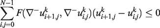
We need a sequence of useful lemmas in order to show that the solution of finite difference scheme (5) converges to the weak solution (6). We first show that the interpolant $U_{N.M}(·,t)$ is TV monotone (We abuse a bit the notation of TV here since our $J(·)$ includes not only a variation term but also an extra L² term).

Lemma 3.2.

$$J(U_{N.M}(·,t_k))\le J(U_{N.M}(·,t)),t_{k-1}\le t\le t_k$$

(19)

Proof. The proof is straightforward. First, it is easy to verify that the continuous variation $J(U_{N.M}(·,t_k))$ equals the discrete variation $J^h(u^k)$ . Then

$$J(U_{N.M}(·,t_k))=J^h(u^k)\le J^h(u^{k-1})=J(U_{N.M}(·,t_{k-1}))$$

Define

$$u(t)=\frac{t-t_{k-1}}{\Delta }t{u}^k+\frac{t_k-t}{\Delta }t{u}^{k-1},t_{k-1}\le t\le t_k$$

To prove (19) is equivalent to prove

$$J^h(u^k)\le J^h(u(t)),t_{k-1}\le t\le t_k$$

Since u^k is the minimizer of the following functional

$$E^h(v)=J^h(v)+\frac{1}{2\Delta t}\left|\right|u^{k-1}-v|{|}^2$$

we have

$$J^h(u^k)+\frac{1}{2\Delta t}\left|\right|u^{k-1}-u^k|{|}^2\le J^h(u(t))+\frac{1}{2\Delta t}||u^{k-1}-u(t)|{|}^2.$$

(20)

For each term in the summation of the L² square term

$$\begin{array}{l}\left|u^{k-1}-u(t)\right|=\left|u^{k-1}-\frac{t-t_{k-1}}{\Delta }t{u}^k+\frac{t_k-t}{\Delta }t{u}^{k-1}\right|\\ =\frac{t-t_{k-1}}{\Delta }t\left|u^k-u^{k-1}\right|\le \left|u^k-u^{k-1}\right|\end{array}$$

Then

$$\frac{1}{2\Delta t}\left|\right|u^{k-1}-u(t)|{|}^2\le \frac{1}{2\Delta t}||u^{k-1}-u^{k-1}|{|}^2$$

We conclude from (20) that

$$J^h(u^k)\le J^h(u(t))$$

Lemma 3.3. Suppose $u^0\in W^{1,1}(\Omega ),f\in L^2(\Omega )$ . Then $\left|\right|\frac{d}{dt}{U}_{N,M}|{|}_{L^2({\Omega }_T)}<C$ for a positive constant C only depending on u⁰ and f.

Proof. From the Euler-Lagrange equation (13)

$$\frac{u^{k-1}-u^k}{\Delta }t=\partial J^h(u^k)$$

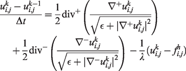
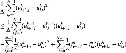
The equation holds element-wise at each index (i, j). For the equation at each index (i, j), we multiply both sides by $u_{i,j}^{k-1}-u_{i,j}^k$ and add the equations for all (i, j). We use inner product notation to write the result in a concise way:

$$〈\frac{u^{k-1}-u^k}{\Delta }t,u^{k-1}-u^k〉=〈\partial J^h(u^k),u^{k-1}-u^k〉$$

By the definition of sub-differential $\partial J^h(u^k)$

$$\begin{array}{l}〈\frac{u^{k-1}-u^k}{\Delta }t,u^{k-1}-u^k〉=〈\partial J^h(u^k),u^{k-1}-u^k〉\\ \le J^h(u^{k-1})-J^h(u^k).\end{array}$$

Note that

$$\frac{d{U}_{N,M}}{dt}=\frac{u^{k-1}-u^k}{\Delta }t,t^{k-1}<t<t_k$$

We have

$$\frac{1}{\Delta }t\left|\right|u^{k-1}-u^k|{|}^2\le J^h(u^{k-1})-J^h(u^k),1\le k\le M$$

Add the above inequalities for $k=1,\cdots ,M$ ,

$${\displaystyle \sum _{k=1}^M\frac{1}{\Delta }}t\left|\right|u^{k-1}-u^k|{|}^2\le J^h(u^0)-J^h(u^M)$$

(21)

It equals

$${\Vert \frac{d{U}_{N,M}}{dt}\Vert }_{L^2({\Omega }_T)}^2\le J^h(u^0)-J^h(u^M)\le J^h(u^0)$$

This completes the proof.

Lemma 3.4. Suppose $u^0,f\in L^2(\Omega )$ . Then $\left|\right|U_{N,M}|{|}_{L^2({\Omega }_T)}\le C$ for a constant C only dependent on f and u⁰.

Proof. We use (17) to bound $U_{N,M}$ . Recall $u_f^0=u^0$ . Letting $C=\max \left\{\right|\left|u_f^0\right||,|\left|f^h\right|\left|\right\}$ , we have

$$\begin{array}{l}\left|\right|U_{N,M}|{|}_{L^2({\Omega }_T)}^2={\displaystyle {\int }_0^T{\Vert U_{N,M}(t)\Vert }_{L^2(\Omega )}^2}\mathrm{d}t\\ ={\displaystyle {\sum }_{k=1}^M{\displaystyle {\int }_{t_{k-1}}^{t_k}{\Vert \frac{(t-t_{k-1})U_{N,M}(·,t_k)+(t_k-t)U_{N,M}(·,t_{k-1})}{\Delta t}\Vert }_{L^2(\Omega )}^2}}\mathrm{d}t\\ \le {\displaystyle \sum _{k=1}^{M}2}{\displaystyle {\int }_{t_{k-1}}^{t_k}\left|\right|}{U}_{N,M}(·,t_k)|{|}_{L^2(\Omega )}^2+||U_{N,M}(·,t_{k-1})|{|}_{L^2(\Omega )}^2\mathrm{d}t\\ \le {\displaystyle \sum _{k=1}^{M}2}{\displaystyle {\int }_{t_{k-1}}^{t_k}\left|\right|}{u}^k|{|}^2+|\left|u^{k-1}\right|{|}^2\mathrm{d}t\le 2T{C}^2\end{array}$$

This completes the proof.

In image analysis, the input image usually does not have much regularity. For example, most natural images do not even have weak derivatives. Therefore, to model images, we introduce the notation of Lipschitz space, and treat images as elements in this space.

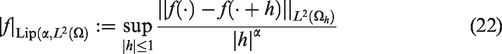
Definition 3.2. Let $\alpha \in (0,1]$ be a real number. A function $f\in \text{Lip}(\alpha ,L^2(\Omega ))$ if $f\in L^2(\Omega )$ and the following quantity

$$|f{|}_{\text{Lip}(\alpha ,L^2(\Omega )}:=\underset{\left|h\right|\le 1}{\sup }\frac{\left|\right|f(·)-f(·+h)|{|}_{L^2({\Omega }_h)}}{|h{|}^{\alpha }}$$

(22)

is finite, where ${\Omega }_h:=\{x\in \Omega ,x+th\in \Omega ,\forall t\in [0,1]\}$ . We let $\left|\right|f|{|}_{\text{Lip}(\alpha ,L^2(\Omega ))}=|\left|f\right|{|}_{L^2(\Omega )}+|f{|}_{\text{Lip}(\alpha ,L^2(\Omega ))}$ .

The parameter α is related to the quantityon mage usually does not have much regularity. For example, most natural ischitz spaces with larger α values.

Lemma 3.5. Define translation operators $T_{1,0}$ and $T_{0,1}$ by

$$\begin{array}{l}(T_{1,0}{u}^k{)}_{i,j}=u_{i+1,j}^k,0\le i,j\le N-1,\\ (T_{0,1}{u}^k{)}_{i,j}=u_{i,j+1}^k,0\le i,j\le N-1\end{array}$$

Then

$$\Vert T_{1,0}{u}^k-u_i^k\Vert \le (|\left|u^0\right|{|}_{\text{Lip}(\alpha ,L^2)}+\left|\right|f|{|}_{\text{Lip}(\alpha ,L^2)})h^{\alpha }$$

and similarly

$$\Vert T_{0,1}{u}^k-u_i^k\Vert \le (|\left|u^0\right|{|}_{\text{Lip}(\alpha ,L^2)}+\left|\right|f|{|}_{\text{Lip}(\alpha ,L^2)})h^{\alpha }$$

Proof. We only prove the first inequality. Recall the Euler-Lagrange equation that

$$\frac{u^{k-1}-u^k}{\Delta t}=\partial J^h(u^k)$$

We write the equation element-wisely as

$$\begin{array}{l}\frac{u_{i,j}^k-u_{i,j}^{k-1}}{\Delta t}=\frac{1}{2}{\text{div}}^{+}\left(\frac{{\nabla }^{+}{u}_{i,j}^k}{\sqrt{\mathrm{ϵ}+|{\nabla }^{+}{u}_{i,j}^k{|}^2}}\right)\\ +\frac{1}{2}{\text{div}}^{-}\left(\frac{{\nabla }^{-}{u}_{i,j}^k}{\sqrt{\mathrm{ϵ}+|{\nabla }^{-}{u}_{i,j}^k{|}^2}}\right)-\frac{1}{\lambda }(u_{i,j}^k-f_{i,j}^h)\end{array}$$

Then subtract the equation at index $(i+1,j)$ from the same equation at index (i, j) for $0\le i\le N-2$ ,

$$\begin{array}{l}\frac{u_{i+1,j}^k-u_{i,j}^k}{\Delta t}-\frac{u_{i+1,j}^{k-1}-u_{i,j}^{k-1}}{\Delta t}\\ =F({\nabla }^{+}{u}_{i+1,j}^k,{\nabla }^{+}{u}_{i,j}^k)+F({\nabla }^{-}{u}_{i+1,j}^k,{\nabla }^{-}{u}_{i,j}^k)\\ -\frac{1}{\lambda }(u_{i+1,j}^k-u_{i,j}^k)+\frac{1}{\lambda }(f_{i+1,j}^h-f_{i,j}^h)\end{array}$$

(23)

where $F({\nabla }^{+}{u}_{i+1,j}^k,{\nabla }^{+}{u}_{i,j}^k)$ is defined by

$$\begin{array}{l}F({\nabla }^{+}{u}_{i+1,j}^k,{\nabla }^{+}{u}_{i,j}^k)=\frac{1}{2}{\text{div}}^{+}\left(\frac{{\nabla }^{+}{u}_{i+1,j}^k}{\sqrt{\mathrm{ϵ}+|{\nabla }^{+}{u}_{i+1,j}^k{|}^2}}\right)\\ -\frac{1}{2}{\text{div}}^{+}\left(\frac{{\nabla }^{+}{u}_{i,j}^k}{\sqrt{\mathrm{ϵ}+|{\nabla }^{+}{u}_{i,j}^k{|}^2}}\right)\end{array}$$

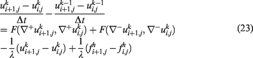
Equation (23) only holds for $0\le i\le N-2,0\le j\le N-1$ . Although equation (23) is not defined for $i=N-1$ , we can set $u_{N+1,j}^k=u_{N,j}^k$ and $f_{N+1,j}=f_{N,j}$ , and equation (23) still holds. we multiply (23) by $u_{i+1,j}^k-u_{i,j}^k$ and add all resulting equations for $0\le i,j\le N-1$ , then

$$\begin{array}{l}\frac{1}{\Delta }t{\displaystyle \sum _{i,j=0}^{N-1}{(u_{i+1,j}^k-u_{i,j}^k)}^2}\\ =\frac{1}{\Delta }t{\displaystyle \sum _{i,j=0}^{N-1}(u_{i+1,j}^{k-1}-u_{i,j}^{k-1})(u_{i+1,j}^k-u_{i,j}^k)}\\ +{\displaystyle \sum _{i,j=0}^{N-1}F}({\nabla }^{+}{u}_{i+1,j}^k,{\nabla }^{+}{u}_{i,j}^k)(u_{i+1,j}^k-u_{i.j}^k)\\ +{\displaystyle \sum _{i,j=0}^{N-1}F}({\nabla }^{-}{u}_{i+1,j}^k,{\nabla }^{-}{u}_{i,j}^k)(u_{i+1,j}^k-u_{i.j}^k)\\ -{\displaystyle \sum _{i,j=0}^{N-1}\frac{1}{\lambda }}(u_{i+1,j}^k-u_{i,j}^k{)}^2\\ +{\displaystyle \sum _{i,j=0}^{N-1}\frac{1}{\lambda }}(f_{i+1,j}^h-f_{i,j}^h)(u_{i+1,j}^k-u_{i,j}^k)\end{array}$$

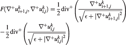
We show next that the second term is no greater than zero. The third term can be proved to be nonpositive similarly. By definition of F,

$$\begin{array}{l}{\displaystyle \sum _{i.j=0}^{N-1}F}({\nabla }^{+}{u}_{i+1,j}^k,{\nabla }^{+}{u}_{i,j}^k)(u_{i+1,j}^k-u_{i,j}^k)\\ ={\displaystyle \sum _{i,j=0}^{N-1}\frac{1}{2}}{\text{div}}^{+}\left(\frac{{\nabla }^{+}{u}_{i+1,j}^k}{\sqrt{\mathrm{ϵ}+|{\nabla }^{+}{u}_{i+1,j}^k{|}^2}}\right)(u_{i+1,j}^k-u_{i,j}^k)\\ -{\displaystyle \sum _{i,j=0}^{N-1}\frac{1}{2}}{\text{div}}^{+}\left(\frac{{\nabla }^{+}{u}_{i,j}^k}{\sqrt{\mathrm{ϵ}+|{\nabla }^{+}{u}_{i,j}^k{|}^2}}\right)(u_{i+1,j}^k-u_{i,j}^k)\end{array}$$

Using summation by part,

$$\begin{array}{l}{\displaystyle \sum _{i.j=0}^{N-1}F}({\nabla }^{+}{u}_{i+1,j}^k,{\nabla }^{+}{u}_{i,j}^k)(u_{i+1,j}^k-u_{i,j}^k)\\ =\frac{1}{2}{\displaystyle \sum _{i,j=0}^{N-1}(u_{i+1,j}^k-u_{i,j}^k)}\\ ·\left({\text{div}}^{+}\left(\frac{{\nabla }^{+}{u}_{i+1,j}^k}{\sqrt{\mathrm{ϵ}+{\nabla }^{+}{u}_{i+1,j}^k{|}^2}}\right)-{\text{div}}^{+}\left(\frac{{\nabla }^{+}{u}_{i,j}^k}{\sqrt{\mathrm{ϵ}+|{\nabla }^{+}{u}_{i,j}^k{|}^2}}\right)\right)\\ =-\frac{1}{2}{\displaystyle \sum _{i,j=0}^{N-1}\left(\left(\frac{{\nabla }^{+}{u}_{i+1,j}^k}{\sqrt{\mathrm{ϵ}+|{\nabla }^{+}{u}_{i+1,j}^k{|}^2}}\right)-\left(\frac{{\nabla }^{+}{u}_{i,j}^k}{\sqrt{\mathrm{ϵ}+|{\nabla }^{+}{u}_{i,j}^k{|}^2}}\right)\right)}\\ ·({\nabla }^{+}{u}_{i+1,j}^k-{\nabla }^{+}{u}_{i,j}^k)-{\displaystyle \sum _{j=0}^{N-1}\frac{|{\nabla }^{+}{u}_{0,j}^k{|}^2}{\sqrt{\mathrm{ϵ}+|{\nabla }^{+}{u}_{0,j}^k{|}^2}}}\end{array}$$

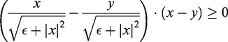
Each term in the first sum is non-negative due to the fact that for any $x,y\in {ℝ}^2$ ,

$$\left(\frac{x}{\sqrt{\mathrm{ϵ}+|x{|}^2}}-\frac{y}{\sqrt{\mathrm{ϵ}+|x{|}^2}}\right)·(x-y)\ge 0$$

By similar arguments, one has

$${\displaystyle \sum _{i,j=0}^{N-1}F}({\nabla }^{-}{u}_{i+1,j}^k,{\nabla }^{-}{u}_{i,j}^k)(u_{i+1,j}^k-u_{i,j}^k)\le 0$$

It follows

$$\begin{array}{l}\frac{1}{\Delta }t{\displaystyle \sum _{i,j=0}^{N-1}{(u_{i+1,j}^k-u_{i,j}^k)}^2}\\ \le \frac{1}{\Delta }t{\displaystyle \sum _{i,j=0}^{N-1}(u_{i+1,j}^{k-1}-u_{i,j}^{k-1})(u_{i+1,j}^k-u_{i,j}^k)}\\ -{\displaystyle \sum _{i,j=0}^{N-1}\frac{1}{\lambda }}(u_{i+1,j}^k-u_{i,j}^k{)}^2+{\displaystyle \sum _{i,j=0}^{N-1}\frac{1}{\lambda }}(f_{i+1,j}^h-f_{i,j}^h)(u_{i+1,j}^k-u_{i,j}^k)\end{array}$$

We rewrite the sums in form of discrete integrals and discrete inner products, and apply Cauchy-Schwartz inequality

$$\begin{array}{l}\frac{1}{\Delta }t\left|\right|T_{1,0}{u}^k-u^k|{|}^2\\ \le \frac{1}{\Delta }t〈T_{1,0}{u}^{k-1}-u^{k-1},T_{1,0}{u}^k-u^k〉\\ -\frac{1}{\lambda }\left|\right|T_{1,0}{u}^k-u^k|{|}^2+\frac{1}{\lambda }〈T_{1,0}f-f,T_{1,0}{u}^k-u^k〉\\ \le \frac{1}{2\Delta t}\left|\right|T_{1,0}{u}^{k-1}-u^{k-1}|{|}^2+\frac{1}{2\Delta t}||T_{1,0}{u}^k-u^k|{|}^2\\ -\frac{1}{2\lambda }\left|\right|T_{1,0}{u}^k-u^k|{|}^2+\frac{1}{2\lambda }||T_{1,0}f-f|{|}^2\end{array}$$

Rearrange and combine similar terms to have

$$\begin{array}{l}(\frac{1}{\Delta }t+\frac{1}{\lambda })\left|\right|T_{1,0}{u}^k-u^k|{|}^2\le \frac{1}{\Delta }t||T_{1,0}{u}^{k-1}-u^{k-1}|{|}^2\\ +\frac{1}{\lambda }\left|\right|T_{1,0}f-f|{|}^2\end{array}$$

(24)

We now prove the following inequality by induction

$$\left|\right|T_{1,0}{u}^k-u^k|{|}^2\le \max \{\left|\right|T_{1,0}{u}^0-u^0|{|}^2,||T_{1,0}f-f|{|}^2\}$$

(25)

It is obvious true for k = 0. Assuming the inequality holds for k. Assuming the inequality holds hods for k by (24). Therefore, one has

$$\begin{array}{l}\left|\right|T_{1,0}{u}^k-u^k\left|\right|\le \left|\right|T_{1,0}{u}^0-u^0\left|\right|+\left|\right|T_{1,0}f-f\left|\right|\\ \le (|\left|u^0\right|{|}_{\text{Lip}(\alpha ,L^2)}+\left|\right|f|{|}_{\text{Lip}(\alpha ,L^2)})h^{\alpha }\end{array}$$

This completes the proof.

We also define a piecewise constant function ${\overline{U}}_{N,M}(·,t)$ in a similar way to the definition of $U_{N.M}(·,t)$ . First we define for $k=0,\dots ,M$

$${\overline{U}}_{N,M}(x,t_k)=u_{i,j}^k,\forall x\in [ih,(i+1)h]\times [jh,(j+1)h].$$

Then we define ${\overline{U}}_{N,M}(·,t)$ for $t_{k-1}\le t\le t_k$ by interpolating $\overline{U}(·,t_{k-1})$ and $\overline{U}(·,t_k)$ :

$$\overline{U}(·,t)=\frac{t-t_{k-1}}{\Delta }t\overline{U}(·,t_k)+\frac{t_k-t}{\Delta }t\overline{U}(·,t_{k-1})$$

We are now ready to show

Lemma 3.6. Suppose $f,u^0\in \text{Lip}(\alpha ,L^2(\Omega ))$ .

$$\begin{array}{l}\left|\right|U_{N,M}-{\overline{U}}_{N,M}|{|}_{L^2({\Omega }_T)}\\ \le C\sqrt{T}(|\left|u^0\right|{|}_{\text{Lip}(\alpha ,L^2)}+\left|\right|f|{|}_{\text{Lip}(\alpha ,L^2)})h^{\alpha }\end{array}$$

for a positive constant C dependent only on f and u⁰.

Proof. Let $g(x,t)=U_{N,M}(x,t)-{\overline{U}}_{N,M}(x,t)$ . For any x, g(x, t) is a linear function of t. A direct calculation shows

$$\begin{array}{l}{\displaystyle {\int }_{t_{k-1}}^{t_k}\left|\right|}g(x,t)|{|}_{L^2(\Omega )}^{2}dt\\ \le \frac{1}{2}\left(\left|\right|g(x,t_k)|{|}_{L^2(\Omega )}^2+||g(x,t_{k-1})|{|}_{L^2(\Omega )}^2\right)(t_k-t_{k-1})\end{array}$$

Adding the inequality for $k=1,\cdots ,M$ , we have

$${\displaystyle {\int }_0^T\left|\right|}g(x,t)|{|}_{L^2(\Omega )}^{2}dt\le \Delta t{\displaystyle \sum _{k=0}^M\left|\right|}g(x,t_k)|{|}_{L^2(\Omega )}^2$$

(26)

Then we only need to bound $\left|\right|g(x,t_k)\left|\right|$ . We note that g(x, t) is a piecewise linear function of x on each sub-grid ${\Omega }_{i,j}:=[ih,(i+1)h]\times [jh,(j+1)h],0\le i,j\le N-1$ for any t. Tedious calculation gives

$$\begin{array}{l}\left|\right|g(x,t_k)|{|}_{L^2(\Omega )}^2\\ ={\displaystyle \sum _{i,j}{\displaystyle {\int }_{{\Omega }_{i,j}}|}}{U}_{N.M}(x,t_k)-{\overline{U}}_{N,M}(x,t_k){|}^2\\ \le {\displaystyle \sum _{i,j}C}{h}^2({\left|u_{i+1,j}^k-u_{i,j}^k\right|}^2+{\left|u_{i,j+1}^k-u_{i,j}^k\right|}^2\\ +{\left|u_{i-1,j}^k-u_{i,j}^k\right|}^2+{\left|u_{i,j-1}^k-u_{i,j}^k\right|}^2)\\ \le C\left({\Vert T_{1,0}{u}^k-u^k\Vert }^2+{\Vert T_{0,1}{u}^k-u^k\Vert }^2\right)\\ \le 2C(|\left|f\right|{|}_{\text{Lip}(\alpha ,L^2)}+\left|\right|u_0|{|}_{\text{Lip}(\alpha ,L^2)}{)}^2{h}^{2\alpha }\end{array}$$

The last line follows from Lemma 3.5. We substitute the bound for the $\left|\right|g(x,t_k)|{|}_{L^2(\Omega )}$ in inequality (26) to complete the proof.

Finally we are ready to prove the main result of this section.

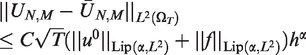
Theorem 3.4. Suppose that $u_0\in W^{1,1}(\Omega ),f\in L^2(\Omega )$ . Furthermore, suppose that $f\in \mathit{Lip}(\alpha ,L^2(\Omega ))$ . If we choose $\Delta t=o(h^{\alpha })$ , then there exists a function $U^{*}$ in $L^2({\Omega }_T)$ so that $U_{N,M}$ converge to $U^{*}$ weakly as $N,M\to \infty$ and $U^{*}$ is the weak solution of (3).

Proof. By Lemma 3.4, there exists a weakly convergent subsequence of $\{U_{N,M},N\ge 1,M\ge 1\}$ in $L^2({\Omega }_T)$ . For convenience, we assume the whole sequence converges to $U^{*}\in L^2({\Omega }_T)$ weakly. We now show $U^{*}$ is the weak solution of the gradient flow (2.1). As the weak solution is unique, the whole sequence $\{U_{N,M},N\ge 1,M\ge 1\}$ converges weakly to $U^{*}$ .

Let us outline the main ideas of the proof. By using Theorem 2.1, we need to show that $U^{*}$ satisfies the following inequality

$$\begin{array}{l}{\displaystyle {\int }_0^s{\displaystyle {\int }_{\Omega }\frac{d}{dt}}}v(v-U^{*})\mathrm{d}x\mathrm{d}t+{\displaystyle {\int }_0^s(J(}v)-J(U^{*}))\mathrm{d}t\\ \ge \frac{1}{2}{\displaystyle {\int }_{\Omega }(v(}x,s)-U^{*}(x,s){)}^2\mathrm{d}x\\ -\frac{1}{2}{\displaystyle {\int }_{\Omega }(v(}x,0)-u_0(x,0){)}^2\mathrm{d}x\end{array}$$

(27)

for all $v\in L^1([0,T],W^{1,1}(\Omega ))$ with $\frac{\partial }{\partial \mathbf{n}}v(x,t)=0$ for all $(t,x)\in [0,T)\times \partial \Omega$ , where

$$J(u)={\displaystyle {\int }_{\Omega }\sqrt{\mathrm{ϵ}+|\nabla u(x,t){|}^2}}dx+\frac{1}{2\lambda }{\displaystyle {\int }_{\Omega }|}f(x,t)-u(u,t){|}^2\mathrm{d}x$$

By the lower semi-continuity of J, we have

$$\begin{array}{l}{\displaystyle {\int }_0^s{\displaystyle {\int }_{\Omega }\frac{d}{dt}}}v(v-U^{*})\mathrm{d}x\mathrm{d}t+{\displaystyle {\int }_0^s(J(}v)-J(U^{*}))\mathrm{d}t\\ \ge \underset{N,M\to \infty }{\lim \inf }[{\displaystyle {\int }_0^s{\displaystyle {\int }_{\Omega }\frac{d}{dt}}}v(v-U_{N,M})\mathrm{d}x\mathrm{d}t\\ +{\displaystyle {\int }_0^s(J(}v)-J(U_{N,M}))\mathrm{d}t]\end{array}$$

(28)

and

$$\begin{array}{l}\underset{N,M\to \infty }{\lim \inf }\frac{1}{2}[{\displaystyle {\int }_{\Omega }(v(}x,s)-U_{N,M}(x,s){)}^2\mathrm{d}x\\ -{\displaystyle {\int }_{\Omega }(v(}x,0)-u_0(x,0){)}^2\mathrm{d}x]\\ \ge \frac{1}{2}[{\displaystyle {\int }_{\Omega }(v(}x,s)-U^{*}(x,s){)}^2\mathrm{d}x-{\displaystyle {\int }_{\Omega }(v(}x,0)-u_0(x,0){)}^2\mathrm{d}x]\end{array}$$

(29)

We now prove the following inequality to finish the proof.

$$\begin{array}{l}{\displaystyle {\int }_0^s{\displaystyle {\int }_{\Omega }\frac{d}{dt}}}v(v-U_{N,M})\mathrm{d}x\mathrm{d}t+{\displaystyle {\int }_0^s(J(}v)-J(U_{N,M}))\mathrm{d}t\\ \ge \frac{1}{2}\left[{\displaystyle {\int }_{\Omega }(v(}x,s)-U_{N,M}(x,s){)}^2\mathrm{d}x-{\displaystyle {\int }_{\Omega }(v(}x,0)-u_0(x,0){)}^2\mathrm{d}x\right]\\ -{\text{Error}}_{N,M}\end{array}$$

where ${\text{Error}}_{N,M}>0$ is an error term that goes to zero as $N,M\to \infty$ . Itan error term that goes to z (cf. Feng and Prohl ⁶ ) that the above inequality is equivalent to

$$\begin{array}{l}{\displaystyle {\int }_0^s{\displaystyle {\int }_{\Omega }\frac{d}{dt}}}{U}_{N,M}(v-U_{N,M})\mathrm{d}x\mathrm{d}t+{\displaystyle {\int }_0^s(J(}v)-J(U_{N,M}))\mathrm{d}t\\ \ge -{\text{Error}}_{N,M}\end{array}$$

(30)

Since $U_{N.M}(·,t)$ is in the finite element space $S_1^0({\Delta }_N)$ associated with triangulation _N , we replace the original $W^{1,1}$ test function $v(·,t)$ in (30) with a test function $v\prime (·,t)$ that is in $L^1([0,T],S_1^0({\Delta }_N))$ and introduce an error $e_{N,M}$ .

$$e_{N.M}={\displaystyle {\int }_0^s{\displaystyle {\int }_{\Omega }\frac{d}{dt}}}{U}_{N,M}(v-v\prime )+J(v)-J(v\prime )$$

It is easy to show $e_{N.M}$ tends to zero as N goes to infinity by standard density argumentation. Thus we only need to prove

$$\begin{array}{l}{\displaystyle {\int }_0^s\left[{\displaystyle {\int }_{\Omega }\frac{d}{\mathrm{d}t}}{U}_{N,M}(v-U_{N,M})\mathrm{d}x+(J(v)-J(U_{N,M}))\right]}\mathrm{d}t\\ \ge -{\text{Error}}_{N,M}\end{array}$$

(31)

for all test functions v in $L^1([0,T],S_1^0({\Delta }_N))$ where ${\text{Error}}_{N,M}$ tends to zero as $N,M\to \infty$ .

Let us verify the key inequality (31). We first prove the inequality for t = t_k. Consider the integrand of the left side of (31) for t = t_k. For a continuous piecewise linear function $v(·,t_k)\in S_1^0({\Delta }_N)$ , assuming $v(·,t_k)={\displaystyle \sum _{i,j}{v}_{i,j}^k}{\varphi }_{i,j}$ , we have

$$\begin{array}{l}J(v(·,t_k))=\frac{h^2}{2}{\displaystyle \sum _{i,j}\sqrt{\mathrm{ϵ}+|{\nabla }^{+}{v}_{i,j}^k{|}^2}}+\frac{h^2}{2}{\displaystyle \sum _{i,j}\sqrt{\mathrm{ϵ}+|{\nabla }^{-}{v}_{i,j}^k{|}^2}}\\ +\frac{1}{2\lambda }{\displaystyle {\int }_{\Omega }(v(}·,t_k)-f{)}^2\end{array}$$

(32)

We need to replace the continuous integral in (32) by a discrete summation with some error. Let ${\tilde{P}}_{N}v(·,t_k)$ be a piecewise constant function defined by

$${\tilde{P}}_{N}v(x,t_k)=v_{i,j}^{k}x\in [ih,(i+1)h]\times [jh,(j+1)h]$$

and $P_{N}f$ be the piecewise constant projection of f as defined in (9). Replacing f and v by P_Nf and ${\tilde{P}}_{N}v$ respectively, we have

$$\begin{array}{l}\frac{1}{2\lambda }{\displaystyle {\int }_{\Omega }(v(}·,t_k)-f{)}^2\\ =\frac{1}{2\lambda }{\displaystyle \sum _{i,j}{(v_{i,j}^k-f_{i,j}^h)}^2}{h}^2\\ +\frac{1}{2\lambda }{\displaystyle {\int }_{\Omega }((}v(·,t_k)-f{)}^2-({\tilde{P}}_{N}v(·,t_k)-P_{N}f{)}^2)\end{array}$$

It is a standard analysis that the second term on the right-hand side converges to zero as $P_{N}f\to f$ and ${\tilde{P}}_{N}v\to v$ in $L^2(\Omega )$ . We omit the detail here. Then

$$\frac{1}{2\lambda }{\displaystyle {\int }_{\Omega }(v(}·,t_k)-f{)}^2=\frac{1}{2\lambda }{\displaystyle \sum _{i,j}{(v_{i,j}^k-f_{i,j}^h)}^2}{h}^2+{\text{Err}}_1$$

where ${\text{Err}}_1$ denotes the error dependent on N that is convergent to zero when $N\to \infty$ . Similarly, we have

$${\displaystyle {\int }_{\Omega }(U_{N,M}(}·,t_k)-f{)}^2={\displaystyle \sum _{i,j}{(u_{i,j}^k-f_{i,j}^h)}^2}{h}^2+{\text{Err}}_2$$

with error term ${\text{Err}}_2$ that converges to zero as $N\to \infty$ by Lemma 3.6.

We remind the reader that that for $t\in (t_{k-1},t_k)$ ,

$$\frac{\mathrm{d}}{\mathrm{d}t}{U}_{N,M}(·,t)=\frac{U_{N,M}(·,t_k)-U_{N,M}(·,t_{k-1})}{\Delta t}$$

(33)

Then

$$\begin{array}{l}{\displaystyle {\int }_{\Omega }\frac{\mathrm{d}}{\mathrm{d}t}}{U}_{N,M}(v-U_{N,M})\mathrm{d}x\\ ={\displaystyle {\int }_{\Omega }\frac{U_{N,M}(·,t_k)-U_{N,M}(·,t_{k-1})}{\Delta t}}(v(·,t_k)-U_{N,M}(·,t_k))\mathrm{d}x\end{array}$$

Replacing $v,U_{N,M}$ by ${\tilde{P}}_{N}v,{\overline{U}}_{N,M}$ respectively, we have

$$\begin{array}{l}{\displaystyle {\int }_{\Omega }\frac{U_{N,M}(·,t_k)-U_{N,M}(·,t_{k-1})}{\Delta t}}(v(·,t_k)-U_{N,M}(·,t_k))\\ ={\displaystyle {\int }_{\Omega }\frac{{\overline{U}}_{N,M}(·,t_k)-{\overline{U}}_{N,M}(·,t_{k-1})}{\Delta t}}({\tilde{P}}_{N}v(·,t_k)\\ -{\overline{U}}_{N,M}(·,t_k))dx+\frac{{\text{Err}}_3}{\Delta t}\\ ={\displaystyle \sum _{i,j}\frac{u_{i,j}^k-u_{i,j}^{k-1}}{\Delta t}}(v_{i,j}-u_{i,j}^k)h^2+\frac{{\text{Err}}_3}{\Delta t}\end{array}$$

where ${\text{Err}}_3$ stands for another error term that can be bounded by Lemma 3.6. Note that we have to use Cauchy-Schwartz inequality to show that ${\text{Err}}_3$ goes to zero at the rate of $h^{\alpha }$ . By one of the assumptions, we know ${\text{Err}}_3/\Delta t\to 0$ when $N\to \infty$ .

We put all the estimates above together to have

$$\begin{array}{l}{\displaystyle {\int }_{\Omega }\frac{\mathrm{d}}{\mathrm{d}t}}{U}_{N,M}(·,t_k)(v(·,t_k)-U_{N,M}(·,t_k))\mathrm{d}x\\ +J(v(·,t_k))-J(U_{N,M}(·,t_k))\\ ={\displaystyle \sum _{i,j}\frac{u_{i,j}^k-u_{i,j}^{k-1}}{\Delta t}}(v_{i,j}^k-u_{i,j}^k)h^2\\ +\frac{1}{2}{\displaystyle \sum _{i,j}\sqrt{\mathrm{ϵ}+|{\nabla }^{+}{v}_{i,j}^k{|}^2}}{h}^2+\frac{1}{2}{\displaystyle \sum _{i,j}\sqrt{\mathrm{ϵ}+|{\nabla }^{-}{v}_{i,j}^k{|}^2}}{h}^2\\ +\frac{1}{2\lambda }{\displaystyle \sum _{i,j}{(v_{i,j}^k-f_{i,j}^h)}^2}{h}^2-\frac{1}{2}{\displaystyle \sum _{i,j}\sqrt{\mathrm{ϵ}+|{\nabla }^{+}{u}_{i,j}^k{|}^2}}{h}^2\\ -\frac{1}{2}\sqrt{\mathrm{ϵ}+|{\nabla }^{-}{u}_{i,j}^k{|}^2}{h}^2-\frac{1}{2\lambda }{\displaystyle \sum _{i,j}{(u_{i,j}^k-f_{i,j}^h)}^2}{h}^2\\ +\frac{{\text{Err}}_3}{\Delta t}+{\text{Err}}_1-{\text{Err}}_2\end{array}$$

Note that the first 7 terms on the right-hand side above are nonnegative by inequality (14) in Lemma 2.1. Then

$$\begin{array}{l}{\displaystyle {\int }_{\Omega }\frac{\mathrm{d}}{\mathrm{d}t}}{U}_{N,M}(·,t_k)(v(·,t_k)-U_{N,M}(·,t_k))dx\\ +J(v(·,t_k))-J(U_{N,M}(·,t_k))\\ \ge \frac{{\text{Err}}_3}{\Delta t}+{\text{Err}}_1-{\text{Err}}_2\end{array}$$

Thus inequality (31) for t = t_k is proved.

Now we consider the inequality when $t\in (t_{k-1},t_k)$ . Note that

$$\begin{array}{l}{U}_{N.M}(·,t)\\ =U_{N.M}(·,t_{k-1})(t_k-t)/\Delta t+U_{N.M}(·,t_k)(t-t_{k-1})/\Delta t\end{array}$$

For $t\in (t_{k-1},t_k)$ , we use (33) to have

$$\begin{array}{l}{\displaystyle {\int }_0^T{\displaystyle {\int }_{\Omega }\frac{\mathrm{d}}{\mathrm{d}t}}}{U}_{N,M}(v(·,t)-U_{N.M}(·.t))\mathrm{d}x\mathrm{d}t\\ ={\displaystyle \sum _{k=1}^M{\displaystyle {\int }_{t_k-1}^{t_k}{\displaystyle {\int }_{\Omega }\frac{U_{N,M}(·,t_k)-U_{N,M}(·,t_{k-1})}{\Delta t}}}}\\ ·(v(·,t)-U_{N,M}(·,t))\mathrm{d}x\mathrm{d}t\\ ={\displaystyle \sum _{k=1}^M{\displaystyle {\int }_{t_k-1}^{t_k}{\displaystyle {\int }_{\Omega }\frac{U_{N,M}(·,t_k)-U_{N,M}(·,t_{k-1})}{\Delta t}}}}\\ ·(v(·,t)-U_{N,M}(·,t_k)\mathrm{d}x\mathrm{d}t+{\text{Err}}_4\end{array}$$

We bound ${\text{Err}}_4$ by

$$\begin{array}{l}\left|{\text{Err}}_4\right|\\ \le {\displaystyle \sum _{k=1}^M{\displaystyle {\int }_{t_k-1}^{t_k}{\displaystyle {\int }_{\Omega }|\frac{U_{N,M}(·,t_k)-U_{N,M}(·,t_{k-1})}{\Delta t}}}}\\ ·(U_{N,M}(·,t_k)-U_{N,M}(·,t_{k-1}))\frac{t_k-t}{\Delta t}|\mathrm{d}x\mathrm{d}t\\ \le {\displaystyle \sum _{k=1}^M{\displaystyle {\int }_{\Omega }|\frac{U_{N,M}(·,t_k)-U_{N,M}(·,t_{k-1})}{\Delta t}}}\\ ·(U_{N,M}(·,t_k)-U_{N,M}(·,t_{k-1}))\mathrm{d}x|\frac{1}{2}\Delta t\\ =\frac{1}{2}\Delta t{\Vert \frac{d{U}_{N,M}}{dt}\Vert }_{{\Omega }_T}^2\\ \le C\Delta t.\end{array}$$

The last line comes from Lemma 3.3.

For the variation term, we have

$$\begin{array}{l}{\displaystyle {\int }_0^{T}J}(v(·,t))-J(U_{N.M}(·,t))\\ ={\displaystyle \sum _{k=1}^M{\displaystyle {\int }_{t_{k-1}}^{t_k}J}}(v(·,t))-J(U_{N.M}(·,t))\mathrm{d}t\\ ={\displaystyle \sum _{k=1}^M{\displaystyle {\int }_{t_{k-1}}^{t_k}J}}(v(·,t))-J(U_{N.M}(·,t_k))\mathrm{d}t+{\text{Err}}_5\end{array}$$

To bound ${\text{Err}}_5$ , we use the monotonicity of the variation term in Lemma 3.2.

$$\left|{\text{Err}}_5\right|={\displaystyle \sum _{k=1}^M{\displaystyle {\int }_{t_{k-1}}^{t_k}J}}(U_{N,M}(·,t))-J(U_{N.M}(·,t_k))\mathrm{d}t$$

By the convexity of J

$$\begin{array}{l}\left|{\text{Err}}_5\right|\\ \le {\displaystyle \sum _{k=1}^M{\displaystyle {\int }_{t_{k-1}}^{t_k}(\frac{t-t_{k-1}}{\Delta }tJ(U_{N.M}(·,t_k))}}\\ +\frac{t_k-t}{\Delta }tJ(J_{N,M}(·,t_{k-1}))-J(U_{N,M}(·,t_k)))\mathrm{d}t\\ ={\displaystyle \sum _{k=1}^M\left(J(U_{N.M}(·,t_{k-1})-J(U_{N.M}(·,t_k))\right)}{\displaystyle {\int }_{t_{k-1}}^{t_k}\frac{t_k-t}{\Delta }}t\mathrm{d}t\\ \le {\displaystyle \sum _{k=1}^M\left(J(U_{N.M}(·,t_{k-1})-J(U_{N.M}(·,t_k))\right)}\Delta t\\ \le \Delta tJ(U_{N.M}(·,0))=\Delta tJ(u^0).\end{array}$$

We conclude that ${\text{Err}}_5$ tends to zero as $\Delta t$ approaches zero. Collecting these results together, we proved inequality (31) for $t_{k-1}\le t\le t_k$ .

Numerical solution of our finite difference scheme

The system (5) of nonlinear equations has been solved by many methods as explained in Vogel and Oman. ⁹ In Dobson and Vogel, ¹⁰ the researchers provided an analysis of a fixed point method proposed in Vogel and Oman ⁹ based on auxiliary variable and functionals and proved that the iterative method converges. In this section, we mainly present another method to show the convergence of the fixed point method. From notation simplicity, we assume the grid size h = 1 in this section that has no influence in the convergence analysis of our algorithm.

First of all, let us explain the fixed point method. Recall that we need to solve $\{u_{i,j}^k,0\le i,j\le N-1\}$ from the following equations

$$\begin{array}{l}\frac{u_{i,j}^k-u_{i,j}^{k-1}}{\Delta }t-\frac{1}{2}{\text{ div}}^{+}\left(\frac{{\nabla }^{+}{u}_{i,j}^k}{\sqrt{\mathrm{ϵ}+|{\nabla }^{+}{u}_{i,j}^k{|}^2}}\right)\\ -\frac{1}{2}{\text{ div}}^{-}\left(\frac{{\nabla }^{-}{u}_{i,j}^k}{\sqrt{\mathrm{ϵ}+|{\nabla }^{-}{u}_{i,j}^k{|}^2}}\right)+\frac{1}{\lambda }(u_{i,j}^k-f_{i,j}^h)=0,\\ 0\le i,j\le N-1\end{array}$$

assuming that we have the solution $\{u_{i,j}^{k-1},0\le i,j\le N-1\}$ . Let us define an iterative algorithm to compute $u_{i,j}^k$ .

Algorithm 4.1. Starting with $v_{i,j}^0=u_{i,j}^{k-1},0\le i,j\le N-1$ , for $\ell =1,2,\cdots ,$ , we compute

$$\frac{v_{i,j}^{\ell }-u_{i,j}^{k-1}}{\Delta }t=\frac{1}{2}{\text{div}}^{+}\left(\frac{{\nabla }^{+}{v}_{i,j}^{\ell }}{\sqrt{\mathrm{ϵ}+|{\nabla }^{+}{v}_{i,j}^{\ell -1}{|}^2}}\right)$$

(34)

$$\begin{array}{l}+\frac{1}{2}{\text{div}}^{-}\left(\frac{{\nabla }^{-}{v}_{i,j}^{\ell }}{\sqrt{\mathrm{ϵ}+|{\nabla }^{-}{v}_{i,j}^{\ell -1}{|}^2}}\right)\\ -\frac{1}{\lambda }(v_{i,j}^{\ell }-f_{i,j}^h),0\le i,j\le N-1\end{array}$$

(35)

together with boundary conditions in (5).

We now show that the iterative solutions $\{v_{i,j}^{\ell },0\le i,j\le N-1\},\ell \ge 0$ converge. Indeed, we first have

Lemma 4.7. There exists a positive constant C dependent only on f and initial values $u_{i,j}^{k-1}$ such that

$$\left|\right|v^{\ell }|{|}^2:={\displaystyle \sum _{i,j}|}{v}_{i,j}^{\ell }{|}^2\le C$$

(36)

for all $\ell \ge 1$ .

Proof. Multiplying $v_{i,j}^{\ell }$ to the equation (34) and summing over $i,j=0,\cdots ,N-1$ , we have

$$\begin{array}{l}\frac{\left|\right|v^{\ell }|{|}^2}{\Delta }t=\frac{1}{\Delta }t{\displaystyle \sum _{i,j}{u}_{i,j}^{k-1}}{v}_{i,j}^{\ell }-\frac{1}{2}{\displaystyle \sum _{i,j}\frac{{\nabla }^{+}{v}_{i,j}^{\ell }{\nabla }^{+}{v}_{i,j}^{\ell }}{\sqrt{\mathrm{ϵ}+|{\nabla }^{+}{v}_{i,j}^{\ell -1}{|}^2}}}\\ -\frac{1}{2}{\displaystyle \sum _{i,j}\frac{{\nabla }^{-}{v}_{i,j}^{\ell }{\nabla }^{-}{v}_{i,j}^{\ell }}{\sqrt{\mathrm{ϵ}+|{\nabla }^{-}{v}_{i,j}^{\ell -1}{|}^2}}}-\frac{1}{\lambda }\left|\right|v^{\ell }|{|}^2+\frac{1}{\lambda }{\displaystyle \sum _{i,j}{f}_{i,j}^h}{v}_{i,j}^{\ell }.\end{array}$$

By using the Cauchy-Schwartz equality, it follows that

$$(\frac{1}{\Delta }t+\frac{1}{\lambda })\left|\right|v^{\ell }|{|}^2\le \frac{1}{\Delta }t|\left|u_{i,j}^{k-1}\right|\left|\right|\left|v^{\ell }\right||+\frac{1}{\lambda }|\left|f^h\right|\left|\right|\left|v^{\ell }\right||$$

Hence, $\left|\right|v^{\ell }\left|\right|$ is bounded by a constant C independent of $\ell$ .

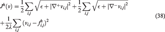
It follows that the sequence of vectors $\{v_{i,j}^{\ell },0\le i,j\le N-1\},\ell \ge 1$ contains a convergent subsequence. Let us say the vectors $v_{i,j}^{{\ell }_k},0\le i,j\le N-1$ converge to $v_{i,j}^{*},0\le i,j\le N-1$ . Next we claim that the whole sequence converges. To prove this claim, we recall the energy functional

$$E^h(v)=J^h(v)+\frac{1}{2\Delta t}{\displaystyle \sum _{i,j}{(v_{i,j}-u_{i,j}^{k-1})}^2}.$$

(37)

where

$$\begin{array}{l}{J}^h(v)=\frac{1}{2}{\displaystyle \sum _{i,j}\sqrt{\mathrm{ϵ}+|{\nabla }^{+}{v}_{i,j}{|}^2}}+\frac{1}{2}{\displaystyle \sum _{i,j}\sqrt{\mathrm{ϵ}+|{\nabla }^{-}{v}_{i,j}{|}^2}}\\ +\frac{1}{2\lambda }{\displaystyle \sum _{i,j}{(v_{i,j}-f_{i,j}^h)}^2}\end{array}$$

(38)

Let us prove the following lemma

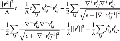
Lemma 4.8. For all $\ell \ge 1$ , we have

$$\frac{1}{2\lambda }\left|\right|v^{\ell }-v^{\ell -1}|{|}^2\le E(v^{\ell -1})-E(v^{\ell }).$$

Proof. Fix $\ell \ge 1$ . For the terms in $E(v^{\ell -1})-E(v^{\ell })$ , we first consider

$$\begin{array}{l}\frac{1}{2\Delta t}{\displaystyle \sum _{i,j}{(v_{i,j}^{\ell -1}-u_{i,j}^{k-1})}^2}-\frac{1}{2\Delta t}{\displaystyle \sum _{i,j}{(v_{i,j}^{\ell }-u_{i,j}^{k-1})}^2}\\ =\frac{1}{2\Delta t}{\displaystyle \sum _{i,j}{(v_{i,j}^{\ell -1}-v_{i,j}^{\ell })}^2}\\ +\frac{1}{\Delta }t{\displaystyle \sum _{i,j}(v_{i,j}^{\ell }-u_{i,j}^{k-1})(v_{i,j}^{\ell -1}-v_{i,j}^{\ell })}.\end{array}$$

(39)

To estimate the second term on the right-hand side of the equation above, we multiply $v_{i,j}^{\ell -1}-v_{i,j}^{\ell }$ to the equation (34) and sum over $i,j=0,\cdots ,N-1$ to have

$$\begin{array}{l}\frac{1}{\Delta }t{\displaystyle \sum _{i,j}(v_{i,j}^{\ell }-u_{i,j}^{k-1})(v_{i,j}^{\ell -1}-v_{i,j}^{\ell })}\\ =-\frac{1}{2}{\displaystyle \sum _{i,j}\frac{{\nabla }^{+}{v}_{i,j}^{\ell }{\nabla }^{+}(v_{i,j}^{\ell -1}-v_{i,j}^{\ell })}{\sqrt{\mathrm{ϵ}+|{\nabla }^{+}{v}_{i,j}^{\ell -1}{|}^2}}}\\ -\frac{1}{2}{\displaystyle \sum _{i,j}\frac{{\nabla }^{-}{v}_{i,j}^{\ell }{\nabla }^{-}(v_{i,j}^{\ell -1}-v_{i,j}^{\ell })}{\sqrt{\mathrm{ϵ}+|{\nabla }^{-}{v}_{i,j}^{\ell -1}{|}^2}}}\\ -\frac{1}{\lambda }{\displaystyle \sum _{i,j}(v_{i,j}^{\ell }-f_{i,j}^h)(v_{i,j}^{\ell -1}-v_{i,j}^{\ell })}.\end{array}$$

Note that it is easy to see

$$\begin{array}{l}-\frac{1}{2}{\displaystyle \sum _{i,j}\frac{{\nabla }^{+}{v}_{i,j}^{\ell }{\nabla }^{+}(v_{i,j}^{\ell -1}-v_{i,j}^{\ell })}{\sqrt{\mathrm{ϵ}+|{\nabla }^{+}{v}_{i,j}^{\ell -1}{|}^2}}}\\ \ge -\frac{1}{4}{\displaystyle \sum _{i,j}\frac{{\nabla }^{+}{v}_{i,j}^{\ell -1}{\nabla }^{+}{v}_{i,j}^{\ell -1}}{\sqrt{\mathrm{ϵ}+|{\nabla }^{+}{v}_{i,j}^{\ell -1}{|}^2}}}+\frac{1}{4}{\displaystyle \sum _{i,j}\frac{{\nabla }^{+}{v}_{i,j}^{\ell }{\nabla }^{+}{v}_{i,j}^{\ell }}{\sqrt{\mathrm{ϵ}+|{\nabla }^{+}{v}_{i,j}^{\ell -1}{|}^2}}}.\end{array}$$

Similar for other term involving ${\nabla }^{-}$ .

Next we consider

$$\begin{array}{l}\frac{1}{2\lambda }{\displaystyle \sum _{i,j}{(v_{i,j}^{\ell -1}-f_{i,j}^h)}^2}-\frac{1}{2\lambda }{\displaystyle \sum _{i,j}{(v_{i,j}^{\ell }-f_{i,j}^h)}^2}\\ =\frac{1}{2\lambda }{\displaystyle \sum _{i,j}(v_{i,j}^{\ell -1}-v_{i,j}^{\ell })(v_{i,j}^{\ell -1}+v_{i,j}^{\ell }-2f_{i,j}^h)}\\ =\frac{1}{2\lambda }{\displaystyle \sum _{i,j}{(v_{i,j}^{\ell -1}-v_{i,j}^{\ell })}^2}\\ +\frac{1}{\lambda }{\displaystyle \sum _{i,j}(v_{i,j}^{\ell }-f_{i,j}^h)(v_{i,j}^{\ell -1}-v_{i,j}^{\ell })}.\end{array}$$

(40)

Finally we can easily verify the following inequality

$$\begin{array}{l}\frac{1}{2}{\displaystyle \sum _{i,j}\sqrt{\mathrm{ϵ}+|{\nabla }^{+}{v}_{i,j}^{\ell -1}{|}^2}}-\frac{1}{2}{\displaystyle \sum _{i,j}\sqrt{\mathrm{ϵ}+|{\nabla }^{+}{v}_{i,j}^{\ell }{|}^2}}\\ \ge \frac{1}{4}{\displaystyle \sum _{i,j}\frac{{\nabla }^{+}{v}_{i,j}^{\ell -1}{\nabla }^{+}{v}_{i,j}^{\ell -1}}{\sqrt{\mathrm{ϵ}+|{\nabla }^{+}{v}_{i,j}^{\ell -1}{|}^2}}}-\frac{1}{4}{\displaystyle \sum _{i,j}\frac{{\nabla }^{+}{v}_{i,j}^{\ell }{\nabla }^{+}{v}_{i,j}^{\ell }}{\sqrt{\mathrm{ϵ}+|{\nabla }^{+}{v}_{i,j}^{\ell -1}{|}^2}}}.\end{array}$$

(41)

Similar for the terms involving ${\nabla }^{-}$ . We now add all equalities and inequalities (39), (40), (41) together to have

$$E(v^{\ell -1})-E(v^{\ell })\ge \frac{1}{2\lambda }{\displaystyle \sum _{i,j}{(v_{i,j}^{\ell -1}-v_{i,j}^{\ell })}^2}.$$

(42)

This completes the proof.

We are now ready to prove the main result in this subsection.

Theorem 4.5. The iterative solutions defined in Algorithm 4.1 converge to the solution of (5) for any fixed $\Delta t>0$ , h > 0, and $k\ge 1$ .

Proof. We have already shown that the iterative solution vectors $\{v_{i,j}^{\ell },0\le i,j\le N-1\}$ have a convergent subsequence $\{v_{i,j}^{{\ell }_n},0\le i,j\le N-1\},n=1,2,\cdots$ to a vector $v^{*}$ . It is easy to see that the energies $E(v^{{\ell }_n}),n\ge 1$ are also convergent to $E(v^{*})$ . By Lemma 4.8, we know that energies $E(v^{\ell })$ are decreasing for all $\ell$ and hence, $E(v^{{\ell }_n+1})$ decrease to $E(v^{*})$ . By using Lemma 4.8 again, we see $\left|\right|v^{{\ell }_n+1}-v^{{\ell }_n}|{|}^2\le 2\lambda (E(v^{{\ell }_n})-E(v^{{\ell }_n+1}))\to 0$ . Thus, $v^{{\ell }_n+1},n\ge 1$ are also convergent to $v^{*}$ . The uniqueness of the solution of (5) implies that $v^{*}$ is the solution vector $\{u_{i,j}^k,0\le i,j\le N-1\}$ .

Numerical experiments

In this section we carry out two numerical experiments. First we demonstrate the convergence of our Algorithm 4.1. Second we apply our algorithm to approximate the solution of (3) on a given time interval. We have implemented the algorithms in MATLAB.

Convergence of Algorithm 4.1

According to Theorem 4.5, given any $\Delta t>0$ , h > 0, $\left\{u_{i,j}^{k-1}\right\}$ , and $\left\{f_{i,j}^h\right\},0\le i,j\le N-1$ , Algorithm 4.1 will generate a convergence sequence ${\left\{v_{i,j}^l\right\}}_l$ , which converges $\left\{u_{i,j}^k\right\}$ of (5).

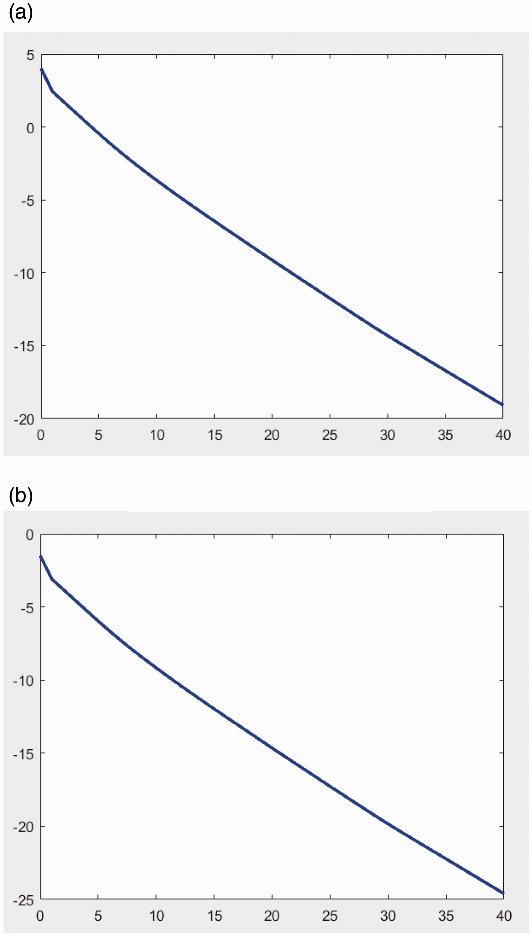
We first generate two random arrays $u^{k-1}=\{u_{i,j}^{k-1},0\le i,j\le 50-1\}$ and $u^k=\{u_{i,j}^k,0\le i,j\le 50-1\}$ using Matlab function rand(). Then according to (5) we can calculate $f^h=\{f_{i,j}^h,0\le i,j\le 50-1\}$ . With $u^{k-1}$ and f^h at hands, we iterate $v^l=\{v_{i,j}^l,0\le i,j\le 50-1\}$ according to Algorithm 4.1, with $v^0=u^{k-1}$ . We show that v^l converges to u^k, as $l\to \infty$ , in a proper norm.

To show that the convergence doesnculate imate small $\Delta t$ , we use the following pramaters: $h=1,\Delta t=2,\mathrm{ϵ}=0.1,\lambda =2$ .

The log of the errors $\left|\right|v^l-u^k|{|}_2$ and $\frac{\left|\right|v^l-u^k|{|}_2}{\left|\right|u^k|{|}_2}$ are plotted against the iteration counts $l=0,1,\cdots ,40$ in Figure 2.

Figure 1.

A triangulation.

Figure 2.

The log profiles of the error and relative errors in Algorithm 4.1, with $h=1,\Delta t=2,\mathrm{ϵ}=0.1,\lambda =2$ . (a) $\log (||v^l-u^k|{|}_2)$ . (b) $\log \left(\frac{\left|\right|v^l-u^k|{|}_2}{\left|\right|u^k|{|}_2}\right)$ .

Approximation of the solution of (3)

One major difficulty to approximate the solution of (3) is, while our algorithm convergences to u^k of (5) for each k, the solutions of (5) and (3) are different. We have proved in Theorem 3.4 that, when the grid size of space domain $h\to 0$ and $\Delta t=o(h^{\alpha })$ , the discrete solution of (5) converges to the weak solution of (3). However, in reality, it is not easy to obtain data of abitrary small h. For example, if f^h is a discrete image, then h is fixed to be 1. Therefore, in this experiment, we fix h = 1, and make $\Delta t$ go to 0.

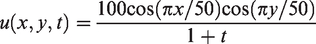
Consider the exact solution of (3)

$$u(x,y,t)=\frac{100\cos (\pi x/50)\cos (\pi y/50)}{1+t}$$

for $(x,y)\in [0,50]\times [0,50]$ and $t\in [0,10]$ . It is straightforward to calculate from the time dependent PDE (3) the corresponding function f with $\lambda >0$ .

We use a uniform mesh $\Delta x=\Delta y=1$ (Figure 1) to discretize the space domain, leading to a set of 51 dent PDE (3) the

$$\widehat{\Omega }=\{(x_i,y_j)|x_i=i,y_j=j,0\le i,j\le 50\}$$

On the time domain, we use a uniform step size $\Delta t_M=10/M$ , and denote ${\widehat{T}}_M={\{t_k=k\Delta t\}}_{k=0}^M$ . We set $u(x,y,0)=100\cos (\pi x/50)\cos (\pi y/50)$ as an initial value. Evolving (5) according to Algorithm 4.1, we get an approximation ${\widehat{u}}_M(x_i,y_j,t_k)$ on grid points $\widehat{\Omega }\times {\widehat{T}}_M$ .

We compare our approximation with the exact solution of (3) at time t = 10, that is, compare ${\widehat{u}}_M(x_i,y_j,10)$ with

$$u(x,y,10)=\frac{100\cos (\pi x/50)\cos (\pi y/50)}{11}$$

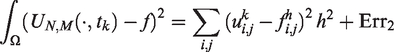
To test the convergence of the algorithm as $\Delta t\to 0$ , we compute on a sequence of decreasing time step sizes $\Delta t_M=10/M$ , where $M=10,11,\cdots ,40$ . The errors are measured in terms of the following norm:

$$\left|\right|u-{\widehat{u}}_M|{|}_{2,t}\stackrel{△}{=}\sqrt{{\displaystyle \sum _{(x_i,y_j)\in \widehat{\Omega }}|}u(x_i,y_j,t)-{\widehat{u}}_M(x_i,y_j,t){|}^2}$$

Theoretically, for t > 0, the error $\left|\right|u-{\widehat{u}}_M|{|}_{2,t}$ will not go to zero, because according to Theorem 4.5, as $M\to \infty ,{\widehat{u}}_M$ goes to the discrete solution of (5) rather than u, which is the exact solution of (3). However, by Theorem 3.4, we should observe that $\left|\right|u-{\widehat{u}}_M|{|}_{2,t}$ converges to a relatively small positive number. It would be ideal, if we could establish an upper bound of the difference between the solutions of (5) and (3). It needs some further study on this matter.

The results of our experiments are illustrated in Figure 3, where the log of the errors $\left|\right|u-{\widehat{u}}_M|{|}_{2,10}$ and $\frac{\left|\right|u-{\widehat{u}}_M|{|}_{2,10}}{\left|\right|u|{|}_{2,10}}$ are plotted as functions of M respectively. We observe that our algorithm converges quickly after M = 30, in all measures.

Figure 3.

This graph demonstrates the convergence. (a) $\log (||u-{\widehat{u}}_M|{|}_{2,10})$ . (b) $\log \left(\frac{\left|\right|u-{\widehat{u}}_M|{|}_{2,10}}{\left|\right|u|{|}_{2,10}}\right)$ .

Conclusions

We end this paper with a few remarks.

Remark 6.3. P. Perona and J. Malik proposed a non-stationary PDE model in Parona and Malik ¹⁵ to remove noises by using anisotropic diffusion. For a given noised image f, we find an improved image u by solving the following non-stationary PDE model with initial value f over time $t\in [0,T)$ :

$$\{\begin{array}{l}\frac{\partial u}{\partial t}=\text{div}(c(|\nabla u{|}^2)\nabla u),\text{ in }\Omega \times (0,T)\hfill \\ \frac{\partial u}{\partial n}=0,\text{ on }\partial \Omega \times (0,T),\hfill \\ u(0,x)=f(x),\text{ in }\Omega ,\hfill \end{array}$$

(43)

where $c(s):[0,+\infty )\mapsto [0,+\infty )$ is a diffusive function which is a decreasing function satisfying $c(0)=1$ and $\underset{s\to +\infty }{\lim }c(s)=0$ . The following is a list of commonly used diffusive functions:

• $c(s)=1/\sqrt{1+s/\lambda }$ which is called Charbonnier diffusivity.

• $c(s)=1/(1+s/\lambda )$ which was used in Parona and Malik.¹⁶ We may call it Perona-Malik diffusivity.

• $c(s)=\exp (-c/\lambda )$ which is the standard Gaussian diffusivity function.

• $c(s)={(1+s/\lambda )}^{\beta -1/2}$ for $\beta \in (0,1/2)$ .

For a fixed c(s), we solve u(T, x) for a large T such that the restored image u(T, x) is a satisfactory one. If we let T sufficiently large, u(T, x) starts a degradation such as some edges are lost or severally blurred.

It is clear when using the Charbonnier diffusivity, i.e., $c(s)=1/\sqrt{\mathrm{ϵ}+s}$ , the PDE in (43) is very similar to the one in (3) with two distinct differences: one is T sufficient $\infty$ and the other one is to use the noised image f as an initial value. Our convergence analysis discussed in the previous two sections can be applied to the PM model with the special diffusive function c(s). In addition, the convexity of anti-derivative of c(s) plays a significant role in our analysis. For other diffusive functions, e.g., Perona-Malik diffusive function, we notice that the function C(s) such that $C\prime (s)=c(s)=1/(1+s/\lambda )$ is not convex when $s>\lambda$ . When $s\le \lambda$ , i.e. $|\nabla u|\le \lambda$ for $t\in [0,T]$ for some T > 0, C(s) is convex and our analysis can be used to show that the corresponding finite difference method is convergent.

Remark 6.4. Our convergence analysis is independent of ϵ. Thus, we can let ϵ = 0. Also, we can replace the integral with coefficient $1/(2\lambda )$ by the boundary integral. Then the time dependent PDE is associated with evolutionary surfaces with prescribed mean curvature as in Lichnewsky and Temam ¹ and Gerhardt. ² Our analysis can be used to show that the corresponding finite difference method for evolutionary surfaces of prescribed mean curvature is convergent to the pseudo-solution.

Remark 6.5. It is interesting to know the convergence rate of the finite difference solution to the weak solution of (3). The convergence rate of the fully discrete finite element solution was established in Feng et al.⁷ under a high regularity assumption on the noised image f, i.e., $f\in L^{\infty }((0,T];W^{1,\infty }(\Omega ))$ and a very high regularity condition on domain d image $\partial \Omega \in C^3$ . In general, an image function may not have such a high regularity. We hope to reduce the assumption on the regularities and give an estimate of convergence rate for the finite element solutions. These have to be left to the interested reader.