Approaching fuzzy sliding mode strategy for automotive suspension based on the view of enhancing ride comfort and vehicle stability

Abstract

This work introduces an algorithm integrated from two component signals called fuzzy sliding mode control (FSMC). This aims to ensure both road holding and ride comfort criteria rather than just one, as mentioned in previous articles. These mentioned criteria are guaranteed based on the design of membership functions and fuzzy rules, while the stability of the sliding mode framework is evaluated through the Lyapunov function. Simulations are performed in the MATLAB-Simulink interface, with four cases corresponding to different road types. According to the calculation results, the displacement and acceleration values of the sprung mass are the smallest once the FSMC method is used to control automotive suspension. In the last case, the wheel can be separated from the road if the automobile has only a passive suspension system or an active suspension system controlled by the proportional integral derivative (PID) algorithm. However, this does not happen when the FSMC algorithm is applied. As a result, the vehicle’s road holding and ride comfort can be ensured in many conditions.

Introduction

The suspension system is used to quell vehicle oscillation. On cars, this system is positioned intermediate to the unsprung mass and the sprung mass. Therefore, it is considered a soft link between these two components. A passive suspension system equipped on most popular cars today usually consists of three main components: springs, shock absorbers, and arms. ¹ Its structure is quite simple, and the price is reasonable. However, it cannot bring smoothness and comfort to passengers in many conditions.

Several modern suspension systems have been invented over the past few years. In, Wang et al. ² introduced semi-active suspension. This suspension system used a magnetorheological damper as an alternative to a linear damper. The stiffness of the magnetorheological damper could be controlled by the magnetic field generated by the controller’s current. ³ The design, development, and commercialization of the semi-active suspension system were analyzed by Soliman and Kaldas. ⁴ Additionally, spring stiffness could be varied by using pneumatic suspension with air springs instead of conventional metal springs. ⁵ This was done based on the change in compressed air pressure inside the chambers of balloons, according to Nguyen. ⁶ The above two solutions could only ensure the ride comfort under certain conditions. To completely overcome this problem, we should use active suspension. According to Sun and Zhao, a hydraulic actuator was included in the active suspension system’s components. ⁷ The hydraulic actuator operation depended on the displacement of the servo valve, which was directed by the voltage signal from a controller. ⁸

Many articles on the subject of suspension control have been published recently. Control methods depend on specific conditions. Shafiei ⁹ proposed using a PID algorithm to control the suspension system, described through a quarter model. The controller parameters in Shafiei ⁹ were tuned by the Ziegler-Nichols classic method. As a result, the efficiency of the controller was not high. The optimal values of the PID controller could be determined by a genetic algorithm (GA), as shown in Metered et al. ¹⁰ According to Metered et al. ¹⁰ the results of GA were only local. In addition, some swarm intelligence algorithms, such as Particle Swarm Optimization (PSO), Artificial Bee Colony (ABC), etc.,^11,12 could also be used to find values for the controller. Unlike GA, these algorithms were more global. We could achieve optimal values for the controller by using optimal search algorithms. However, these values were fixed and could not be changed under different conditions. Based on this idea, Han et al. ¹³ and Ding et al. ¹⁴ used the Fuzzy Logic Control (FLC) method to adjust the controller coefficients according to different conditions flexibly. Combining PID and GA, PSO, ABC, and FLC algorithms could bring high efficiency to Single Input and Single Output (SISO) objects. We should apply the Linear Quadratic Regulator (LQR) technique instead if the system had many objects that need to be controlled. According to Nguyen et al. the purpose of the LQR solution was to minimize the cost function. ¹⁵ In general, these two methods were only suitable for linear systems.

In fact, the vehicle oscillation is nonlinear. As a consequence of this, it is necessary to make use of more complicated algorithms in order to control the suspension system. In, Chen et al. ¹⁶ proposed a nonlinear suspension model controlled by the SMC technique. If the quarter model including hydraulic actuators was used, the SMC technique would have five state variables. ¹⁷ The number of state variables would depend on the model used in studies. ¹⁸ According to Nguyen, ¹⁹ the system was only stable, once the object moved along the sliding surface to return to equilibrium. Therefore, the sliding surface was considered an essential criterion. The results in Chen et al. ¹⁶ Nguyen, ¹⁷ and Konieczny et al. ¹⁸ only referred to the change in displacement, velocity, and acceleration of the sprung mass over time. When using the SMC algorithm to control the suspension system, car oscillation was reduced compared to the passive suspension system. In other words, the smoothness and comfort of the car could be improved when applying this algorithm. However, stability and road holding were not mentioned in these studies. Compared to control algorithms for linear systems such as PID and LQR, the SMC technique brought higher efficiency. Despite this, the “chattering” phenomena could still be observed when using the SMC method. ²⁰ This was a characteristic phenomenon and was challenging to eliminate. This issue had the potential to bring about a decline in the system’s overall quality. The SMC algorithm should be integrated with another algorithm to solve this phenomenon. In, Zhang et al. ²¹ combined the SMC and the PD algorithm to improve the controller’s efficiency. In, Nguyen and Nguyen ²² introduced the combination between the SMC algorithm and PID algorithm with a state multivariable model. If an SMC hybrid integrated controller was used, the “chattering” phenomenon could also be significantly improved. ²³ There were several solutions used to improve the performance of sliding mode controllers. According to Pang et al. ²⁴ the vehicle suspension’s dynamic performance could be improved using the Adaptive Sliding Mode Based Fault Tolerant (ASMFT) controller. The controller in Pang et al. ²⁴ had two controlled objects: center displacement and roll angle. Research results showed that displacement, acceleration, roll angle, and roll acceleration all decreased when applying the I-without fault controller. A similar solution was shown in Pang et al. ²⁵ for automotive suspension systems with sensor faults and parameter uncertainties. In, Hsiao and Wang ²⁶ proposed using an integrated controller called Self-tuning Fuzzy Sliding Mode (STFSM) to direct the damping of active suspension. Road surface excitation in Hsiao and Wang ²⁶ was used according to ISO 8608, while the ride comfort level was evaluated according to ISO 2631-1. Nguyen ²⁷ introduced an algorithm integrating SM, PI, and Fuzzy. Hence, it was called FSMPIF. The final control signal in Nguyen ²⁷ was combined from component signals: PI and Fuzzy. This PI controller was adjusted by another Fuzzy solution, while the original Fuzzy controller had three inputs (including the output signal of SMC). Some control methods for other nonlinear systems were also applied to suspension system models, such as H-infinity Sliding Mode Control (H-SMC) robust control,^28–30 adaptive SMC,^31–33 backstepping SMC, ³⁴ and neural network SMC.^35,36

Recently, some new sliding mode control technique applications for suspension systems have been published. Chen et al. ³⁷ applied the adaptive sliding mode control technique to reject disturbances to improve the vertical stability of the air suspension. This technique also effectively ensured horizontal stability, according to Maciejewski et al. ³⁸ In addition, applying the SMC technique combined with a disturbance observer also helped improve the stability of high-speed rail vehicles, according to Shi et al. ³⁹ An improvement of the SMC algorithm for suspension systems that were affected by uncertainties was shown by Liu and Chen. ⁴⁰ In, Jiang et al. ⁴¹ introduced a Fuzzy self-tuning method for the sliding mode controller of an active suspension system, which used a feedforward neural network. A combination between SMC and PID was also established by Nguyen et al. ⁴² The control parameters in Nguyen et al. ⁴² were optimally calculated by loop algorithms instead of dynamically adjusted, such as Nguyen ¹⁷ and Jiang et al. ⁴¹ The “chattering” phenomenon was significantly mitigated when combining the SMC algorithm with other algorithms. In addition, the performance of the system had also improved. However, there were still some limitations relating to selecting optimal parameters for adaptive SMC and robust SMC controllers or designing appropriate fuzzy rules and membership functions for the Fuzzy SM controller. Simulation results showed that these algorithms had the potential to help ensure smooth driving for cars. Like the above, the results in reference [20–41] only mentioned the change in vehicle body acceleration and displacement (ride comfort) without mentioning road holding. In some cases, the interaction between the road and wheels may decline, although the ride comfort was still guaranteed. The cause of this was the excessive operation of the suspension hydraulic actuator. Ignoring the results of road holding was a significant drawback when investigating suspension control.

Road holding and ride comfort are two essential criteria that should be used when evaluating active suspension systems. The articles mentioned above often only consider the criteria of ride comfort (based on changes in acceleration and displacement of sprung mass or roll angle and roll acceleration), but ignore the influence of road holding. In this work, we introduce using an integrated controller, Fuzzy-SMC, to control the suspension system. Fuzzy rules and membership functions are designed to guarantee road holding and ride comfort. This new contribution to the article can overcome the problem mentioned above. The article structure is divided into four sections: an introduction section, a material and method section, a results and discussion section, and a conclusion section. The specific contents are presented below.

Material and method

Advanced control theory

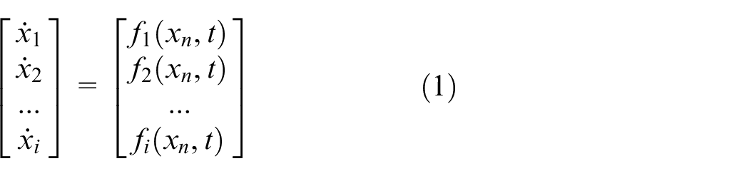
Given a nonlinear system described by equation (1) as below.

$$\left[\begin{array}{c}{\stackrel{·}{x}}_1\hfill \\ \multicolumn{1}{c}{{\stackrel{·}{x}}_2}\\ \multicolumn{1}{c}{...}\\ \multicolumn{1}{c}{{\stackrel{·}{x}}_i}\end{array}\right]=\left[\begin{array}{c}{f}_1(x_n,t)\hfill \\ \multicolumn{1}{c}{f_2(x_n,t)}\\ \multicolumn{1}{c}{...}\\ \multicolumn{1}{c}{f_i(x_n,t)}\end{array}\right]$$

(1)

According to Lyapunov’s Theorem: If it is possible to find a positive definite function $V\left(x\right)=V(x_1,x_2,...,x_i)$ such that its derivative following the difference equation of the disturbing movement ${\stackrel{·}{x}}_1=f(x_1,x_2,...,x_i)$ is negatively defined, then the motion that is not disturbed would be asymptotically stable.

The quadratic structure of the function V(x) is described in equation (2).

$$V\left(x\right)=\frac{1}{2}\sum _{n=1}^i\sum _{m=1}^i{q}_{\mathrm{nm}}{x}_n{x}_m$$

(2)

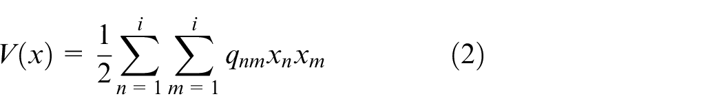
According to Sylvester’s Theorem: The quadratic form of V(x) is considered to be positive definite when the primary diagonal determinants of the symmetric matrix R are all required to have positive values.

$$V\left(x\right)>0\iff \mathit{R}>0$$

(3)

where:

$$\mathit{R}={\left[r_{\mathrm{nm}}\right]}_{n\times m}$$

(4)

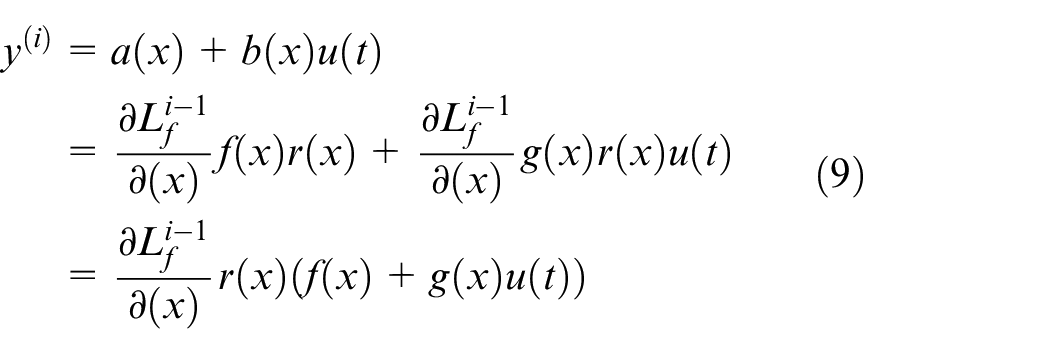
Consider the degree i nonlinear object defined by the equation (5).

$$\{\begin{array}{c}\stackrel{·}{x}=f\left(x\right)+g\left(x\right)u\left(t\right)\hfill \\ \multicolumn{1}{c}{y=r\left(x\right)}\end{array}$$

(5)

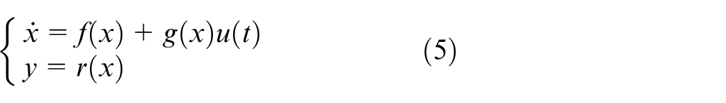
with: x is the system’s state vector, and y is the output signal.

Take i times the derivatives of the output signal, we get equation (6):

$$y^{\left(i\right)}=a\left(x\right)+b\left(x\right)u\left(t\right)=L_f^{i}h\left(x\right)+L_g{L}_f^{i-1}r\left(x\right)u\left(t\right)$$

(6)

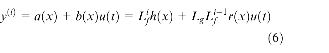
where:

$$L_f^k=\frac{\partial L_f^{k-1}}{\partial \left(x\right)}f\left(x\right)$$

(7)

$$L_g=\frac{\partial g\left(x\right)}{\partial \left(x\right)}$$

(8)

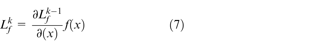
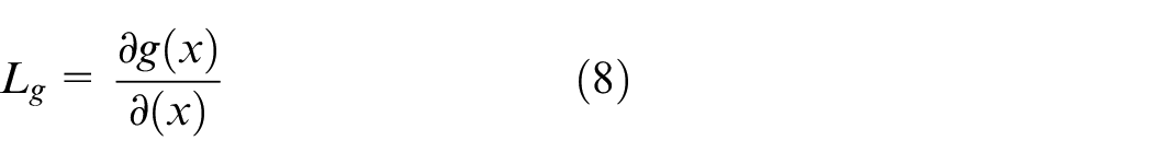
Substitute equations (12) and (13) into equation (6), we get equation (9):

$$\begin{array}{c}\multicolumn{1}{c}{y^{\left(i\right)}=a\left(x\right)+b\left(x\right)u\left(t\right)}\\ \multicolumn{1}{c}{=\frac{\partial L_f^{i-1}}{\partial \left(x\right)}f\left(x\right)r\left(x\right)+\frac{\partial L_f^{i-1}}{\partial \left(x\right)}g\left(x\right)r\left(x\right)u\left(t\right)}\\ \multicolumn{1}{c}{=\frac{\partial L_f^{i-1}}{\partial \left(x\right)}r\left(x\right)(f\left(x\right)+g\left(x\right)u\left(t\right))}\end{array}$$

(9)

Let e(t) represent the difference between the setpoint (y _sp ) and output (y) signals:

$$e\left(t\right)=y_{\mathrm{sp}}\left(t\right)-y\left(t\right)$$

(10)

The generated control signal must make the system and error function tend to be zero when t tends to be infinite. This is described in equation (11).

$$0=\underset{t\to \infty }{lim}{x}_{k+1}\left(t\right)=\underset{t\to \infty }{lim}\frac{d^{k}y\left(t\right)}{d{t}^k}=-\underset{t\to \infty }{lim}\frac{d^{k}e\left(t\right)}{d{t}^k}0\le k\le n-1$$

(11)

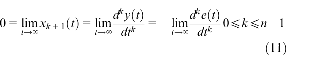
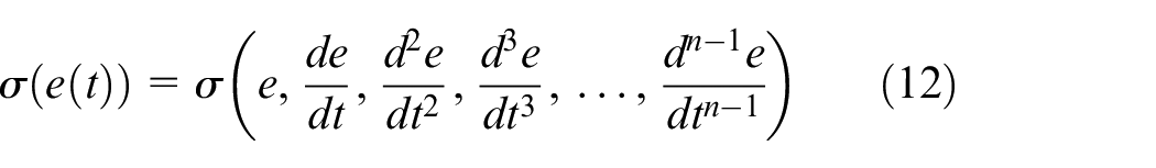
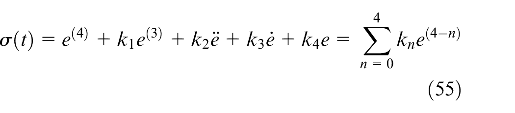
Consider a smooth function describing the error e(t) and its derivatives as equation (12) such that the solution e(t) of the equation σ(t) = 0 (*) satisfies condition equation (11). The function σ(t) that satisfies this is called the sliding surface of the system (Figure 1). The equation (13) describes a linear sliding surface, with the coefficients k _i being real constants. This type of the sliding surface is commonly used in research on automobile suspension control.^{43, 44} However, the sliding surface used in this study (as the equation (55)) is more complicated.

$$\sigma \left(e\left(t\right)\right)=\sigma (e,\frac{\mathrm{de}}{\mathrm{dt}},\frac{d^{2}e}{d{t}^2},\frac{d^{3}e}{d{t}^3},\dots ,\frac{d^{n-1}e}{d{t}^{n-1}})$$

(12)

$$\sigma \left(t\right)=e^{(i-1)}+k_1{e}^{(i-2)}+\dots +k_{i-2}\stackrel{·}{e}+k_{i-1}e$$

(13)

$$K\left(s\right)=s^{i-1}+k_1{s}^{i-2}+\dots +k_{i-2}s+k_{i-1}$$

(14)

Figure 1.

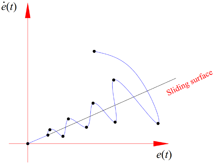
Sliding surface.

To ensure that the solutions of (*) satisfy condition equation (11), the coefficients k _i of the sliding surface equation (13) should be referenced from equation (14). The polynomial equation (14) must be a Hurwitz polynomial; that is, K(s) is real when s is real, and the roots of K(s) have real parts that are zero or negative, where s is a variable of the polynomial equation (14).

A system is asymptotically stable if and only σ(t) → 0, that is:

$$\sigma \left(t\right)\frac{d\sigma \left(t\right)}{\mathrm{dt}}<0\mathrm{or}\mathrm{sgn}\left(\sigma \left(t\right)\right)\frac{d\sigma \left(t\right)}{\mathrm{dt}}<0$$

(15)

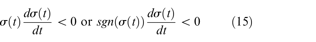
This is simply understood as when σ(t) > 0, the controller must reduce σ(t) and vice versa. As a result, σ(t) will approach zero. The equation (15) becomes the sliding condition that needs to be designed for the controller.

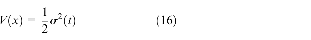
The Lyapunov function is chosen according to ⁴⁵ as below:

$$V\left(x\right)=\frac{1}{2}{\sigma }^2\left(t\right)$$

(16)

The derivative of V(x):

$$\stackrel{·}{V}\left(x\right)=\sigma \left(t\right)\stackrel{·}{\sigma }\left(t\right)<0$$

(17)

To the system become stable, it is necessary to select the control signal u(t) so that the derivative of V(x) is negative. Taking the derivative of equation (13), we get equation (18):

$$\stackrel{·}{\sigma }\left(t\right)=e^{\left(i\right)}+k_1{e}^{(i-1)}+\dots +k_{i-2}\stackrel{··}{e}+k_{i-1}\stackrel{·}{e}$$

(18)

Combining equations (10) and (18), we obtain equation (19):

$$\stackrel{·}{\sigma }\left(t\right)=y_{\mathrm{sp}}^{\left(i\right)}-y^{\left(i\right)}+k_1{e}^{(i-1)}+\dots +k_{i-2}\stackrel{··}{e}+k_{i-1}\stackrel{·}{e}$$

(19)

Combining equations (6) with (19), the derivative of the sliding surface is rewritten as follows:

$$\begin{array}{c}\multicolumn{1}{c}{\stackrel{·}{\sigma }\left(t\right)=y_{\mathrm{sp}}^{\left(i\right)}-[a\left(x\right)+b\left(x\right)u\left(t\right)]+k_1{e}^{(i-1)}}\\ \multicolumn{1}{c}{+\dots +k_{i-2}\stackrel{··}{e}+k_{i-1}\stackrel{·}{e}}\end{array}$$

(20)

To satisfy condition equation (17), we choose:

$$\stackrel{·}{\sigma }\left(t\right)=-\mathrm{Psgn}\left(\sigma \right)$$

(21)

where: P is a positive constant.

Therefore, the equation (17) becomes:

$$\stackrel{·}{V}\left(x\right)=-P\sigma \mathrm{sgn}\left(\sigma \right)<0\forall \sigma \ne 0$$

(22)

Combining equations (20) and (21), the control signal u(t) is determined by the equation (23).

$$\begin{array}{c}\multicolumn{1}{c}{u\left(t\right)=\frac{1}{b\left(x\right)}}\\ \multicolumn{1}{c}{[-a\left(x\right)+y_{\mathrm{sp}}^{\left(i\right)}+k_1{e}^{(i-1)}+\dots +k_{i-2}\stackrel{··}{e}+k_{i-1}\stackrel{·}{e}+\mathrm{Psgn}\left(\sigma \right)]}\end{array}$$

(23)

Control model

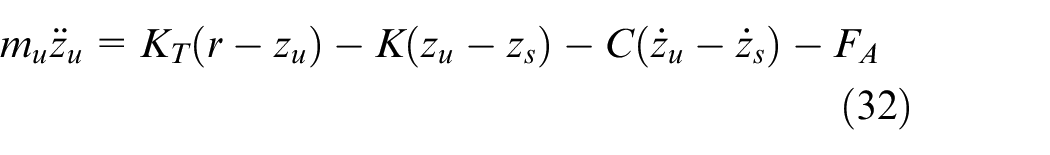
In order to describe the vehicle oscillation, a dynamics model must be developed. This model comprises two different masses: sprung and unsprung masses (Figure 2). The masses are corresponded by two degrees of freedom (DOF), z _s and z _u , respectively. The hydraulic actuator can make the impact force, denoted by F _A , which acts on both masses.

Figure 2.

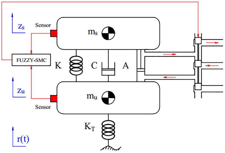
A quarter-dynamics model.

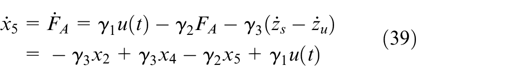
The equation system describing the vehicle oscillation is presented as follows:

$$F_K+F_C+F_A-F_{\mathrm{ims}}=0$$

(24)

$$F_{\mathrm{KT}}-F_K-F_C-F_A-F_{\mathrm{imu}}=0$$

(25)

where: F _K is spring force, F _C is damper force, F _KT is tire force, F _ims is the inertia force (sprung mass), F _imu is the inertia force (unsprung mass), K is the spring stiffness coefficient, C is damper coefficient, K _T is the tire spring stiffness coefficient, m _s is sprung mass, m _u is unsprung mass, and r(t) is roughness on the road.

$$F_K=-K(z_s-z_u)$$

(26)

$$F_C=-C({\stackrel{·}{z}}_s-{\stackrel{·}{z}}_u)$$

(27)

$$F_{\mathrm{KT}}=-K_T(z_u-r)$$

(28)

$$F_{\mathrm{ims}}=m_s{\stackrel{··}{z}}_s$$

(29)

$$F_{\mathrm{imu}}=m_u{\stackrel{··}{z}}_u$$

(30)

Substitute equations (26)–(30), into equations (24) and (35), we get:

$$m_s{\stackrel{··}{z}}_s=K(z_u-z_s)+C({\stackrel{·}{z}}_u-{\stackrel{·}{z}}_s)+F_A$$

(31)

$$m_u{\stackrel{··}{z}}_u=K_T(r-z_u)-K(z_u-z_s)-C({\stackrel{·}{z}}_u-{\stackrel{·}{z}}_s)-F_A$$

(32)

A linear equation (33) provides a close approximation to the description of the active suspension actuator. Nguyen ¹⁹ is one responsible for carrying out the linearization operation. This equation is also used in a few other publications; therefore, its utility is widespread.^{17, 22, 46}

$${\stackrel{·}{F}}_A={\gamma }_{1}u\left(t\right)-{\gamma }_2{F}_A-{\gamma }_3({\stackrel{·}{z}}_s-{\stackrel{·}{z}}_u)$$

(33)

where: γ ₁ , γ ₂ , and γ ₃ are the parameters of the linearized actuator. Their values should be referred to in.^19,22

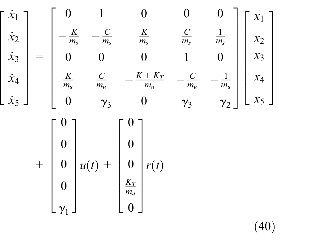
Let state variables:

$$\begin{array}{c}\multicolumn{1}{c}{x_1=z_s}\\ \multicolumn{1}{c}{x_2={\stackrel{·}{z}}_s}\\ \multicolumn{1}{c}{x_3=z_u}\\ \multicolumn{1}{c}{x_4={\stackrel{·}{z}}_u}\\ \multicolumn{1}{c}{x_5=F_A}\end{array}$$

(34)

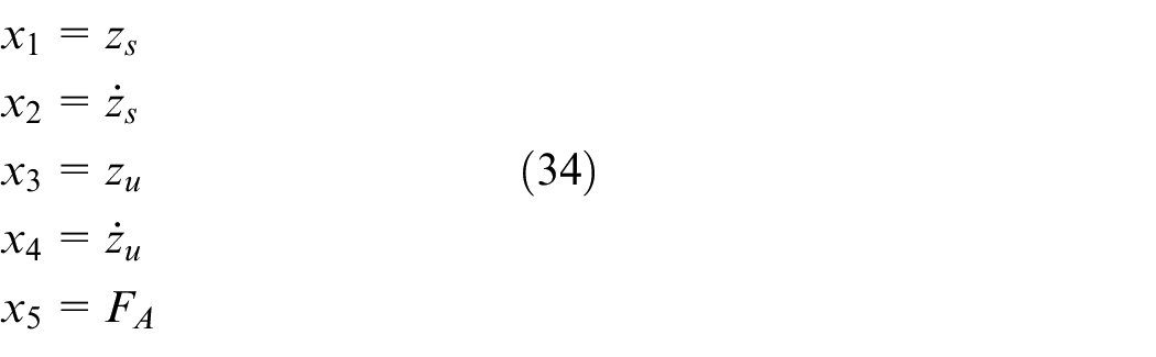
Using the differentiation of state variables:

$${\stackrel{·}{x}}_1={\stackrel{·}{z}}_s=x_2$$

(35)

$$\begin{array}{c}\multicolumn{1}{c}{{\stackrel{·}{x}}_2={\stackrel{··}{z}}_s=\frac{K}{m_s}(z_u-z_s)+\frac{C}{m_s}({\stackrel{·}{z}}_u-{\stackrel{·}{z}}_s)+\frac{F_A}{m_s}}\\ \multicolumn{1}{c}{=\frac{1}{m_s}(-K{x}_1-C{x}_2+K{x}_3+C{x}_4+x_5)}\end{array}$$

(36)

$${\stackrel{·}{x}}_3={\stackrel{·}{z}}_u=x_4$$

(37)

$$\begin{array}{c}\multicolumn{1}{c}{{\stackrel{·}{x}}_4={\stackrel{··}{z}}_u=\frac{K_T}{m_u}(r-z_u)-\frac{K}{m_u}(z_u-z_s)-\frac{C}{m_u}({\stackrel{·}{z}}_u-{\stackrel{·}{z}}_s)-\frac{F_A}{m_u}}\\ \multicolumn{1}{c}{=\frac{1}{m_u}[K{x}_1+C{x}_2-(K+K_T)x_3-C{x}_4-x_5]}\end{array}$$

(38)

$$\begin{array}{c}\multicolumn{1}{c}{{\stackrel{·}{x}}_5={\stackrel{·}{F}}_A={\gamma }_{1}u\left(t\right)-{\gamma }_2{F}_A-{\gamma }_3({\stackrel{·}{z}}_s-{\stackrel{·}{z}}_u)}\\ \multicolumn{1}{c}{=-{\gamma }_3{x}_2+{\gamma }_3{x}_4-{\gamma }_2{x}_5+{\gamma }_{1}u\left(t\right)}\end{array}$$

(39)

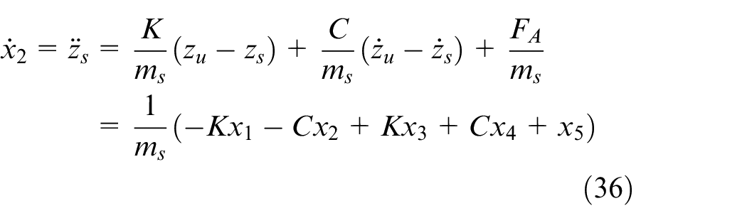
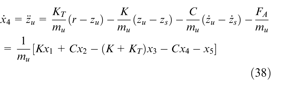
The equation system describing oscillations of the car equations (31) and (32) can be rewritten as follows:

$$\begin{array}{c}\multicolumn{1}{c}{\left[\begin{array}{c}\begin{array}{c}{\stackrel{·}{x}}_1\hfill \\ \multicolumn{1}{c}{{\stackrel{·}{x}}_2}\end{array}\hfill \\ \multicolumn{1}{c}{{\stackrel{·}{x}}_3}\\ \multicolumn{1}{c}{{\stackrel{·}{x}}_4}\\ \multicolumn{1}{c}{{\stackrel{·}{x}}_5}\end{array}\right]=\left[\begin{array}{ccccc}0\hfill & 1\hfill & 0\hfill & 0\hfill & 0\hfill \\ \multicolumn{1}{c}{-\frac{K}{m_s}}& -\frac{C}{m_s}\hfill & \frac{K}{m_s}\hfill & \frac{C}{m_s}\hfill & \frac{1}{m_s}\hfill \\ \multicolumn{1}{c}{0}& 0\hfill & 0\hfill & 1\hfill & 0\hfill \\ \multicolumn{1}{c}{\frac{K}{m_u}}& \frac{C}{m_u}\hfill & -\frac{K+K_T}{m_u}\hfill & -\frac{C}{m_u}\hfill & -\frac{1}{m_u}\hfill \\ \multicolumn{1}{c}{0}& -{\gamma }_3\hfill & 0\hfill & {\gamma }_3\hfill & -{\gamma }_2\hfill \end{array}\right]\left[\begin{array}{c}\begin{array}{c}{x}_1\hfill \\ \multicolumn{1}{c}{x_2}\end{array}\hfill \\ \multicolumn{1}{c}{x_3}\\ \multicolumn{1}{c}{x_4}\\ \multicolumn{1}{c}{x_5}\end{array}\right]}\\ \multicolumn{1}{c}{+\left[\begin{array}{c}\begin{array}{c}0\hfill \\ \multicolumn{1}{c}{0}\end{array}\hfill \\ \multicolumn{1}{c}{0}\\ \multicolumn{1}{c}{0}\\ \multicolumn{1}{c}{{\gamma }_1}\end{array}\right]u\left(t\right)+\left[\begin{array}{c}\begin{array}{c}0\hfill \\ \multicolumn{1}{c}{0}\end{array}\hfill \\ \multicolumn{1}{c}{0}\\ \multicolumn{1}{c}{\frac{K_T}{m_u}}\\ \multicolumn{1}{c}{0}\end{array}\right]r\left(t\right)}\end{array}$$

(40)

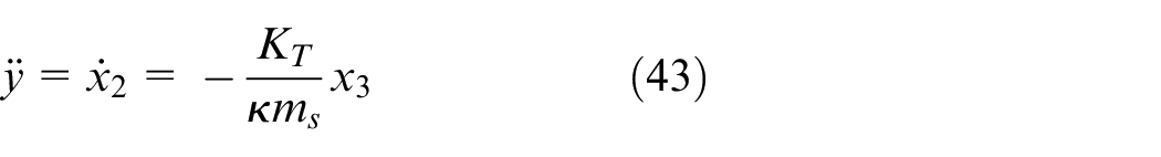
The value of the vehicle body displacement is assumed to be the controller’s output signal throughout this research. Therefore:

$$y=z_s=x_1$$

(41)

Taking the first to the fifth derivative of the output signal:

$$\stackrel{·}{y}={\stackrel{·}{x}}_1=x_2$$

(42)

$$\stackrel{··}{y}={\stackrel{·}{x}}_2=-\frac{K_T}{\kappa m_s}{x}_3$$

(43)

$$y^{\left(3\right)}=-\frac{K_T}{\kappa m_s}{\stackrel{·}{x}}_3=-\frac{K_T}{\kappa m_s}{x}_4$$

(44)

$$y^{\left(4\right)}=-\frac{K_T}{\kappa m_s}{\stackrel{·}{x}}_4=-\frac{K_T}{\kappa m_s{m}_u}[K{x}_1+C{x}_2-(K+K_T)x_3-C{x}_4-x_5]$$

(45)

$$\begin{array}{c}\multicolumn{1}{c}{y^{\left(5\right)}=-\frac{K_T}{\kappa m_s{m}_u}[K{\stackrel{·}{x}}_1+C{\stackrel{·}{x}}_2-(K+K_T){\stackrel{·}{x}}_3-C{\stackrel{·}{x}}_4-{\stackrel{·}{x}}_5]}\\ \multicolumn{1}{c}{=-\frac{K_T}{\kappa m_s{m}_u}\left\{\begin{array}{c}K{x}_2+C\left[\frac{1}{m_s}(-K{x}_1-C{x}_2+K{x}_3+C{x}_4+x_5)\right]-(K+K_T)x_4\hfill \\ \multicolumn{1}{c}{-C\left[\frac{1}{m_u}[K{x}_1+C{x}_2-(K+K_T)x_3-C{x}_4-x_5]\right]-[-{\gamma }_3{x}_2+{\gamma }_3{x}_4-{\gamma }_2{x}_5+{\gamma }_{1}u\left(t\right)]}\end{array}\right\}}\\ \multicolumn{1}{c}{=\frac{K_T}{\kappa m_s{m}_u}\left[\begin{array}{c}(\frac{\mathrm{KC}}{m_s}+\frac{\mathrm{KC}}{m_u})x_1+(\frac{C^2}{m_s}+\frac{C^2}{m_u}-K-{\gamma }_3)x_2\hfill \\ \multicolumn{1}{c}{+(-\frac{\mathrm{KC}}{m_s}-\frac{(K+K_T)C}{m_u})x_3+(-\frac{C^2}{m_s}-\frac{C^2}{m_u}+(K+K_T)+{\gamma }_3)x_4}\\ \multicolumn{1}{c}{+(-\frac{C}{m_s}-\frac{C}{m_u}-{\gamma }_2)x_5+{\gamma }_{1}u\left(t\right)}\end{array}\right]}\end{array}$$

(46)

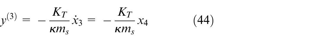
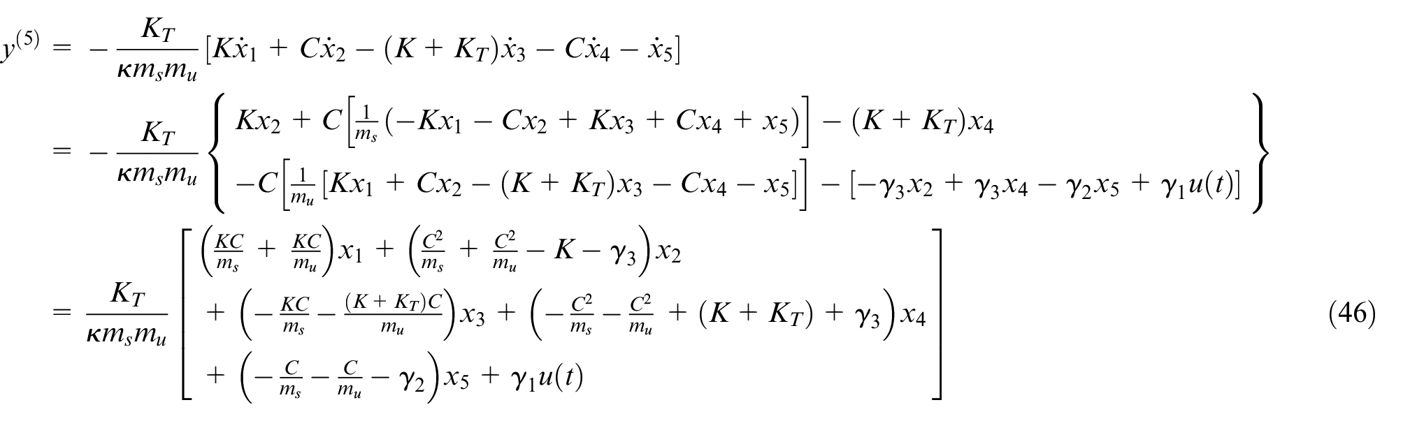
Note: The equation (43) is obtained by linearizing the relationship between the acceleration of the sprung mass and the unsprung mass. This was shown in Nguyen et al., ¹⁹ where κ is the scaling factor.

Let:

$$b_1=\frac{K_T}{\kappa m_s{m}_u}$$

(47)

$$b_2=\frac{K_T{\gamma }_1}{\kappa m_s{m}_u}$$

(48)

$$a_1=\frac{\mathrm{KC}}{m_s}+\frac{\mathrm{KC}}{m_u}$$

(49)

$$a_2=\frac{C^2}{m_s}+\frac{C^2}{m_u}-K-{\gamma }_3$$

(50)

$$a_3=-\frac{\mathrm{KC}}{m_s}-\frac{(K+K_T)C}{m_u}$$

(51)

$$a_4=-\frac{C^2}{m_s}-\frac{C^2}{m_u}+(K+K_T)+{\gamma }_3$$

(52)

$$a_5=-\frac{C}{m_s}-\frac{C}{m_u}-{\gamma }_2$$

(53)

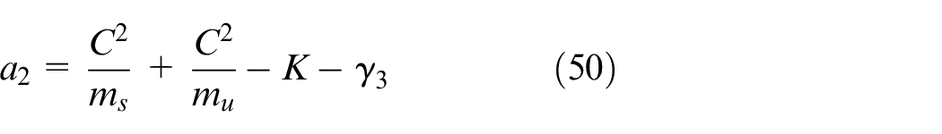
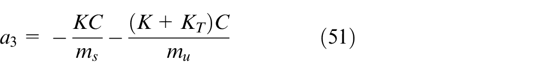
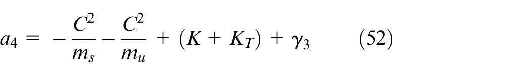
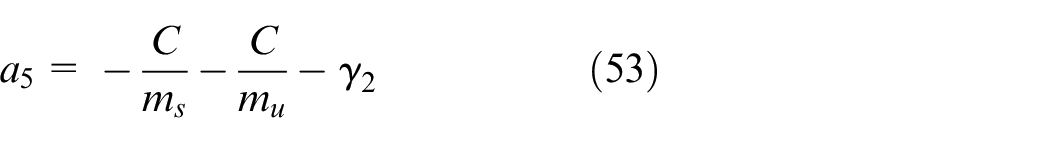
The fifth derivative signal can be rewritten as below:

$$y^{\left(5\right)}=\sum _{n=1}^5{b}_1{a}_n{x}_n+b_{2}u\left(t\right)$$

(54)

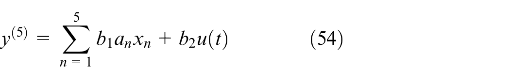
According to equation (13), the sliding surface of this model can be given as equation (55).

$$\sigma \left(t\right)=e^{\left(4\right)}+k_1{e}^{\left(3\right)}+k_2\stackrel{··}{e}+k_3\stackrel{·}{e}+k_{4}e=\sum _{n=0}^4{k}_n{e}^{(4-n)}$$

(55)

The first control signal of the controller has the form:

$$\begin{array}{c}\multicolumn{1}{c}{u_1\left(t\right)=\frac{\kappa m_s{m}_u}{K_T{\gamma }_1}}\\ \multicolumn{1}{c}{[y_s^{\left(5\right)}-\sum _{n=1}^5{a}_n{x}_n+\sum _{n=1}^4{k}_n{e}^{(4-n)}+\mathrm{Psgn}\left(\sum _{n=0}^4{k}_n{e}^{(4-n)}\right)]}\end{array}$$

(56)

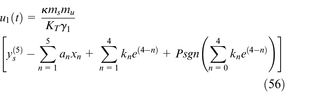
In this work, the values of k _i and P are chosen according to previous simulation experience.

In order to limit the “chattering” phenomenon, the FLC method is combined with the SMC technique. This algorithm takes two input signals, including vehicle displacement and acceleration. The membership function of the FLC algorithm is illustrated in Figure 3. We use triangular and trapezoidal membership functions to describe the fuzzification process. The triangular function has a linear slope. Therefore, it can respond quickly to changes in external conditions. Regarding the first input (sprung mass acceleration), membership functions are divided equally from −10 to +10 m/s². This is a typical value range for vehicle body acceleration when oscillating. This value range is determined based on simulation results from some previous studies.^43–51 If the input value is outside this range, the degree of membership will be equal to one (trapezoidal function). About the second input (sprung mass displacement), the process of building membership functions is performed similarly to the first input. The stable value range is from −80 to +80 mm. If the body displacement exceeds this range, the car will experience strong vibrations. Therefore, the degree of membership is chosen to be equal to one (trapezoidal function) when the input exceeds ±80 mm.

Figure 3.

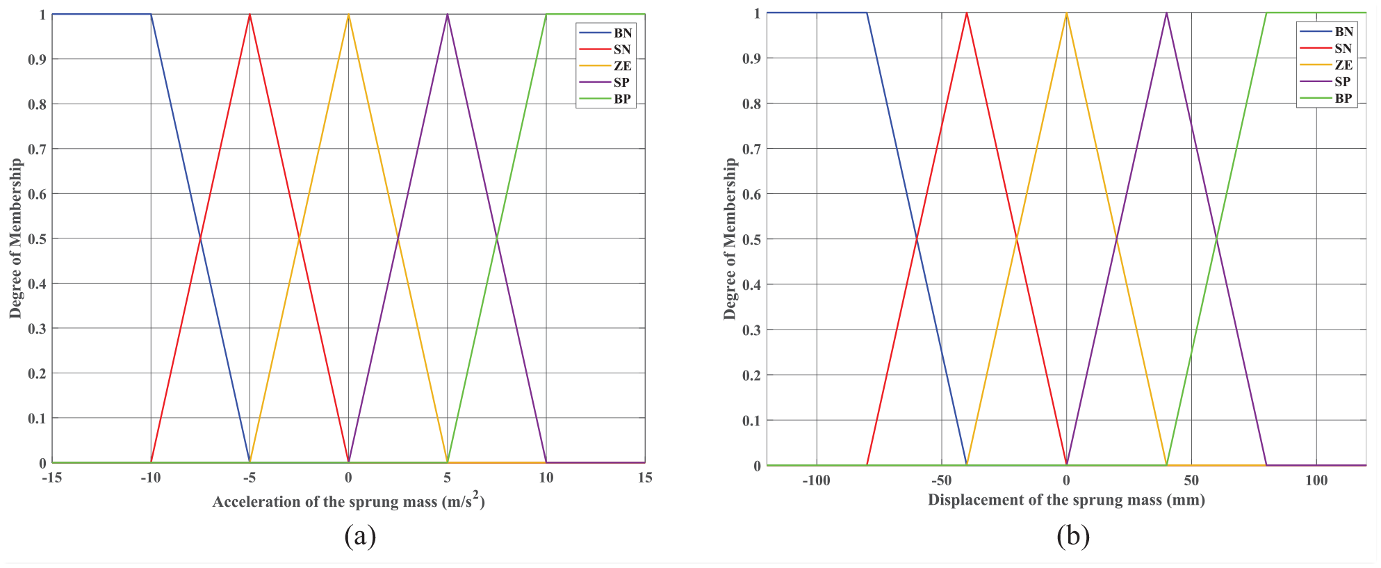
Membership function: (a) The first input. (b) The second input.

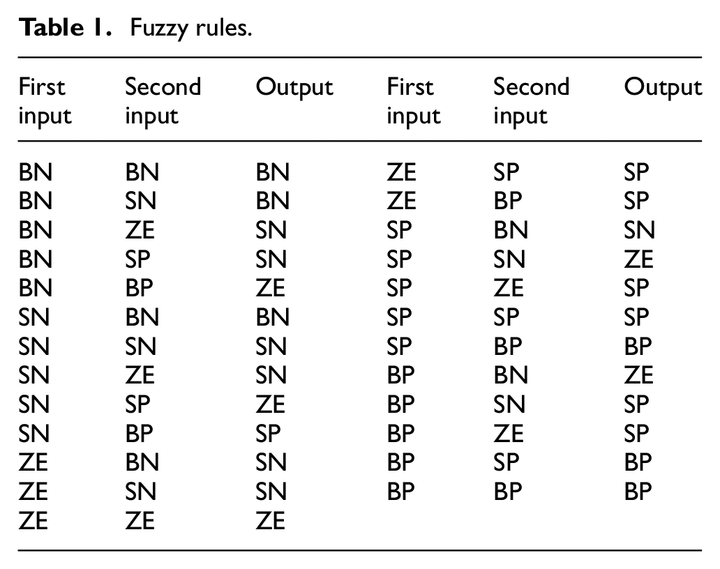
Fuzzy law is designed according to the author’s point of view (Figure 4). The second control signal is determined through the defuzzification process. The content of this process is described in Table 1, including big negative (BN), small negative (SN), zero (ZE), small positive (SP), and big positive (BP). The rule in Table 1 shows that if the displacement and acceleration are large, the control signal needs to be significant. The controller should only generate a correspondingly small signal if displacement and acceleration are small. In cases where one input value is significant, and the other is small, the control signal should be maintained at a relative level. If displacement and acceleration are negligible, the control signal may be zero.

$$u_2\left(t\right)=\mathrm{defuzz}(z_s,{\stackrel{··}{z}}_s)$$

(57)

Figure 4.

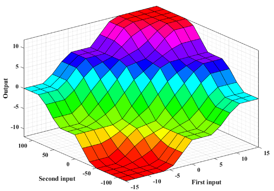
Rule surface.

Table 1.

Fuzzy rules.

First input	Second input	Output	First input	Second input	Output
BN	BN	BN	ZE	SP	SP
BN	SN	BN	ZE	BP	SP
BN	ZE	SN	SP	BN	SN
BN	SP	SN	SP	SN	ZE
BN	BP	ZE	SP	ZE	SP
SN	BN	BN	SP	SP	SP
SN	SN	SN	SP	BP	BP
SN	ZE	SN	BP	BN	ZE
SN	SP	ZE	BP	SN	SP
SN	BP	SP	BP	ZE	SP
ZE	BN	SN	BP	SP	BP
ZE	SN	SN	BP	BP	BP
ZE	ZE	ZE

The final control signal of the controller is combined from component signals, u ₁ (t) and u ₂ (t).

$$u\left(t\right)=u_1\left(t\right)+u_2\left(t\right)$$

(58)

Figure 5 shows a diagrammatic representation of the control system. After completing the controller’s design, the simulation process will be carried out.

Figure 5.

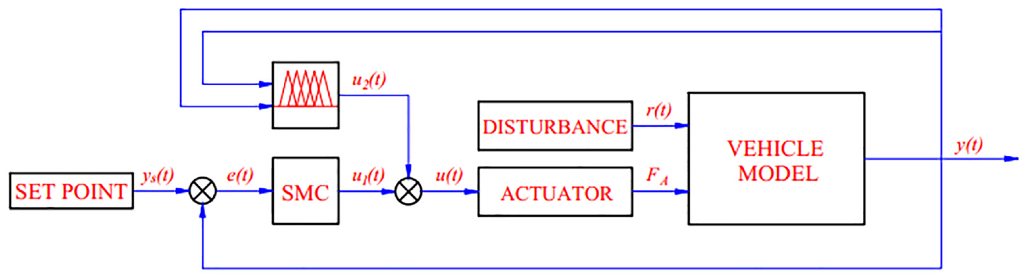
Control system schematic.

Simulation and result

Simulation condition

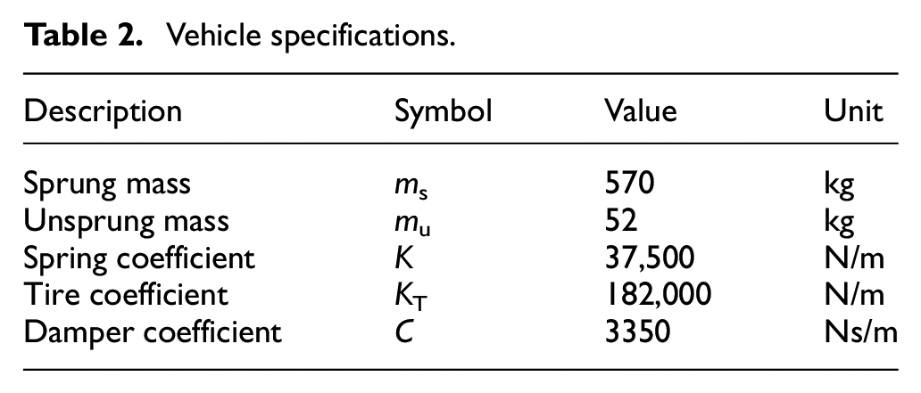
Simulation is done to evaluate the controller quality. This is the numerical simulation that is done in the MATLAB interface. The reference vehicle parameters are given in Table 2.

Table 2.

Vehicle specifications.

Description	Symbol	Value	Unit
Sprung mass	m s	570	kg
Unsprung mass	m u	52	kg
Spring coefficient	K	37,500	N/m
Tire coefficient	K T	182,000	N/m
Damper coefficient	C	3350	Ns/m

The simulation will perform four cases corresponding to four road types (Figure 6). In each case, three situations were examined: a car using passive suspension, active suspension controlled by the PID algorithm, and active suspension controlled by the FSMC algorithm. The problem’s output results are the body displacement and acceleration values. Besides, the change of the dynamic load is also taken into account. These values are compared with each other.

Figure 6.

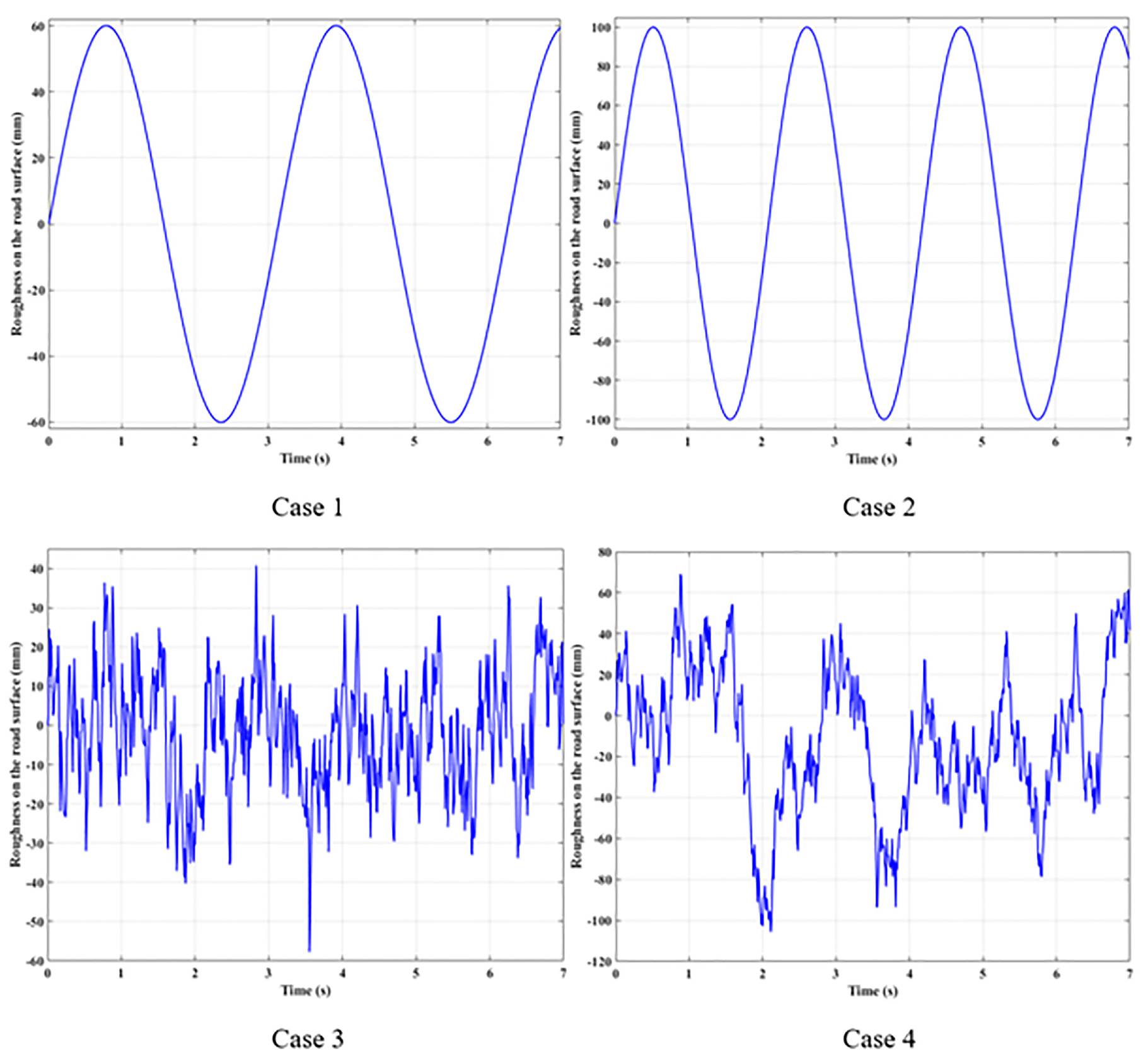
Roughness on the road surface.

Result and discussion

Simulation results are shown in four cases.

The first case

In the first case, the road excitation is sine waves of small amplitude. This is a form of periodic transform with a low frequency. This excitation form is often used in control problems for suspension systems. Simulation results are shown in four cases.

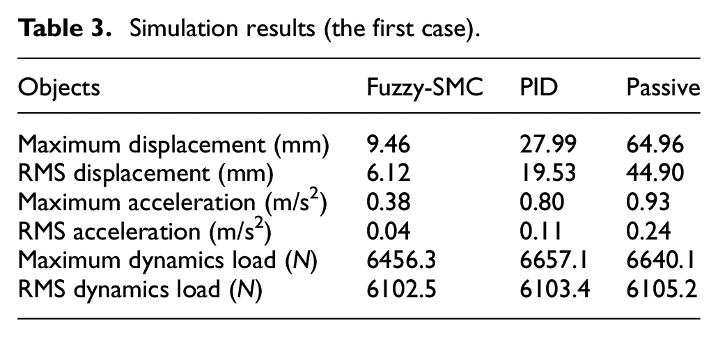
Figure 7 gives information about the vehicle body displacement over simulation time. This value tracks to follow the excitation signal from the road. The peak displacement value may be up to 9.46, 27.99, and 64.96 mm, corresponding to investigated situations: FMSC, PID, and Passive. For continuous oscillations, the average values should also be considered. The average displacement values are able to be calculated according to the root mean square (RMS) criteria. According to RMS, the oscillation value when the car only uses the mechanical suspension system is quite large, up to 44.90 mm (Passive), corresponding to the time t = 7 s. If the PID controller directs active suspension, this value drops sharply to 19.53 mm. Besides, the FMSC algorithm can reduce this value, even more, only 13.63% compared to the first situation.

Figure 7.

Sprung mass displacement (Case 1).

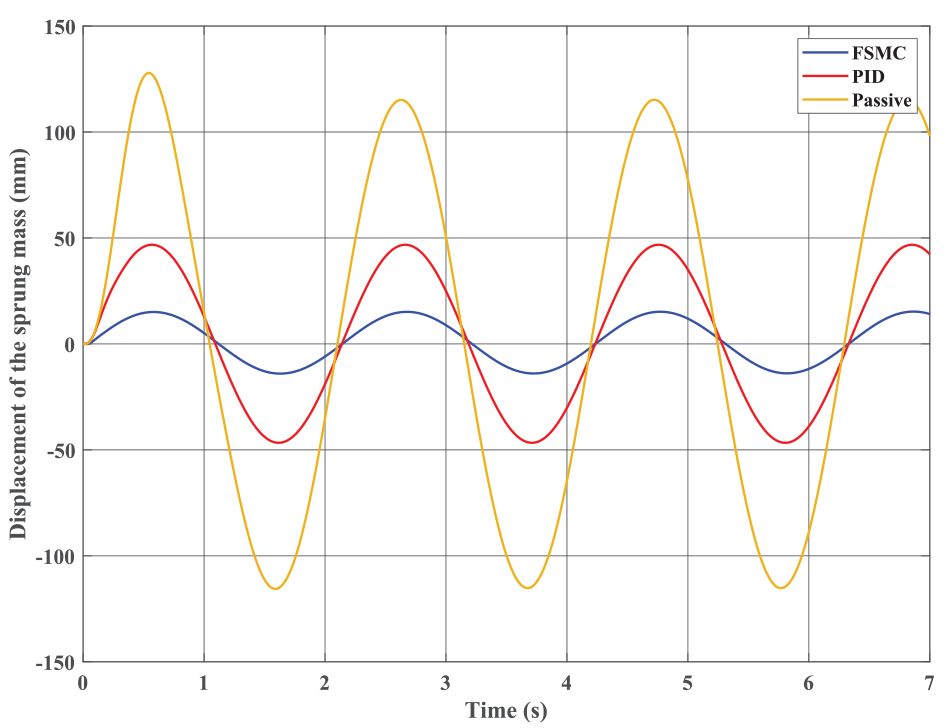
The vehicle body acceleration is used to assess vehicle smoothness. The change in vehicle body acceleration is shown in Figure 8. According to these results, maximum acceleration values achieved in the first phase are 0.93  m/s² (Passive), 0.80 m/s² (PID), and 0.38 m/s² (FSMC). This value gradually decreases in subsequent phases and changes periodically. For the third situation (FSMC), the vehicle body acceleration can overshoot every time the oscillation phase changes. However, this overshoot is very small. It almost does not affect the comfort and smoothness of the vehicle. According to the RMS criterion, the value of the acceleration in this case is 0.24, 0.11, and 0.04 m/s². The difference between the last and first situations is quite significant, six times each other. The comfort and smoothness of the third situation would be better.

Figure 8.

Sprung mass acceleration (Case 1).

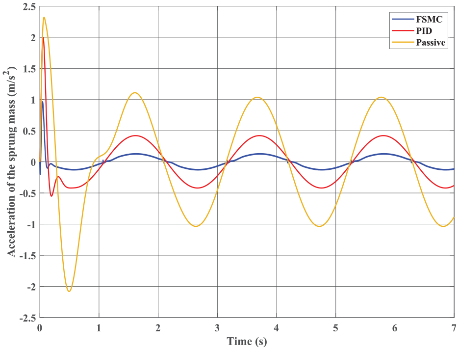
When the vehicle body oscillates, a wheel load changes called the dynamic load. The wheel will grip the road better if the dynamic load change is small. Conversely, the holding between the wheel and the road will worsen if the dynamic load is more considerable. Once the value of the dynamic force approaches zero, the wheel can be detached from the road. The holding between the wheel and the road will be terminated at that time. The wheel can no longer take forces from the road surface so instability may occur. The variation of the dynamic load is shown in Figure 9. This graph has a form that closely resembles the acceleration of the car. Accordingly, the change in dynamic force in the third situation is the smallest; it tends to be asymptotic to the initial static load. For the other two situations, the dynamic load variation is more considerable. However, the difference, in this case, is not much. The simulation results of the first case are summarized in Table 3.

Figure 9.

Dynamics load (Case 1).

Table 3.

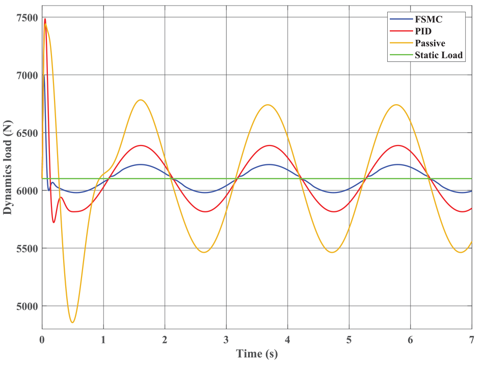
Simulation results (the first case).

Objects	Fuzzy-SMC	PID	Passive
Maximum displacement (mm)	9.46	27.99	64.96
RMS displacement (mm)	6.12	19.53	44.90
Maximum acceleration (m/s2)	0.38	0.80	0.93
RMS acceleration (m/s2)	0.04	0.11	0.24
Maximum dynamics load (N)	6456.3	6657.1	6640.1
RMS dynamics load (N)	6102.5	6103.4	6105.2

The second case

In the second case, the sine-shaped road is continued to be used. According to Figure 6, its amplitude and frequency are larger than in the first case.

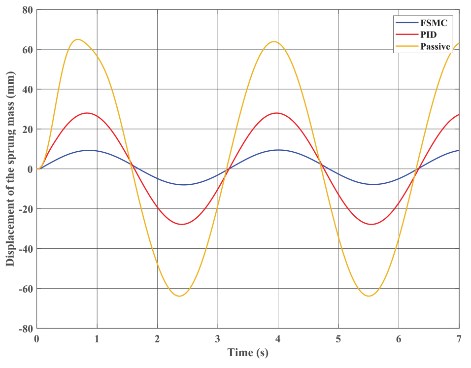
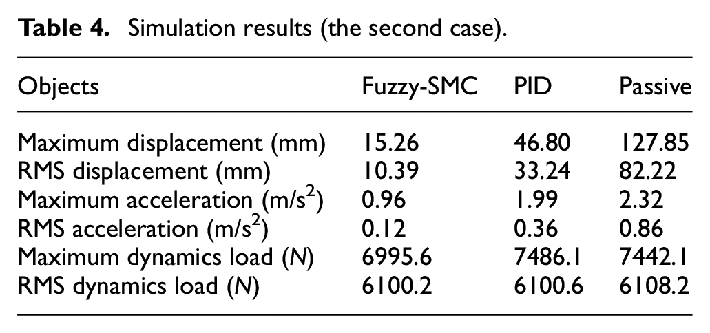
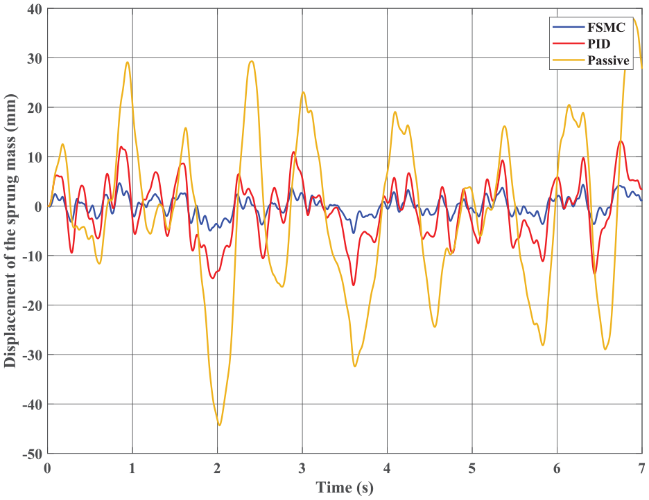
The vehicle body displacement in the second case is more extensive than in the first case (Figure 10). The reason for this is that the excitation of the pavement has a larger amplitude. The peak value of displacement corresponding to three situations is 127.85, 46.80, and 15.26 mm. Their mean values are also proportional to the peak values, reaching 82.22, 33.24, and 10.39 mm. Once the vehicle’s body moves too much, the ride comfort can be affected. This is true for situations where the car utilizes only passive suspension. Once active suspension controlled by the FSMC technique is used, the vehicle’s comfort will be much better.

Figure 10.

Sprung mass displacement (Case 2).

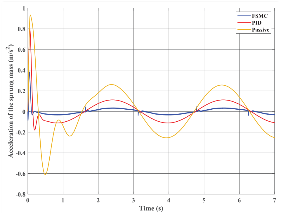
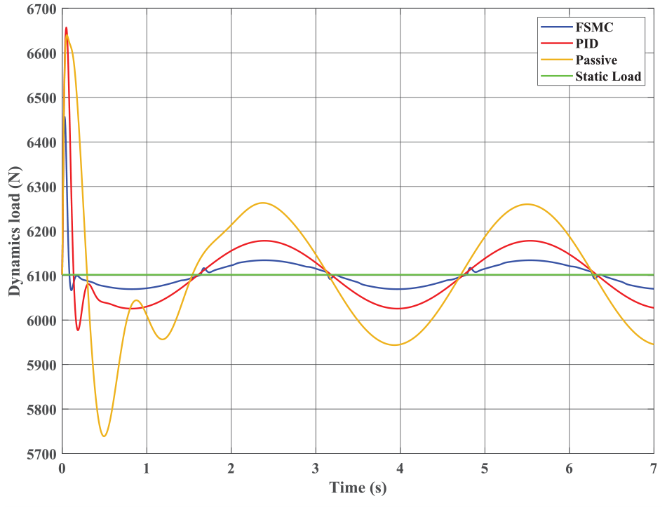
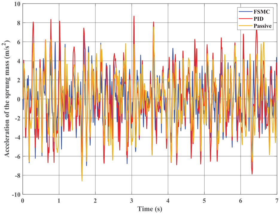
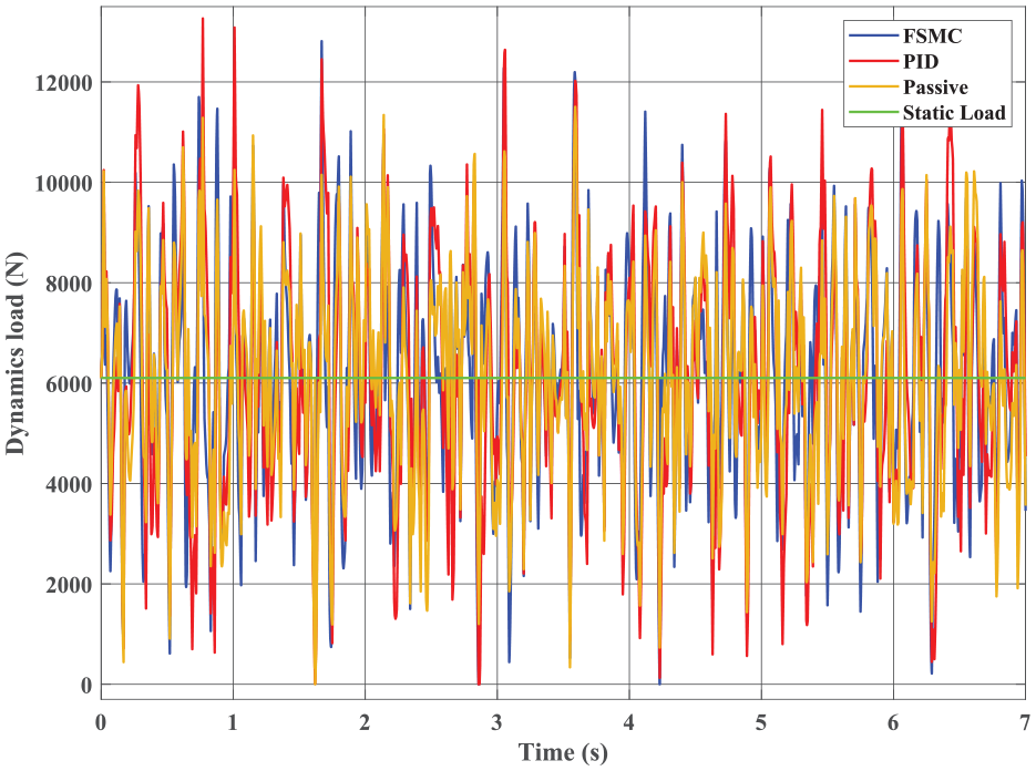
The change in car body acceleration with time in the second case is also more significant than in the first case (Figure 11). Compared with the vehicle using mechanical suspension, if active suspension with the FSMC algorithm is used, its peak value and RMS values are only 41.38% and 13.95%, respectively. Overshoot does not affect the ride comfort much. The dynamics load change in the second case is also not large (Figure 12). In general, the wheel can still interact well with the road surface. The destabilization has not happened yet.

Figure 11.

Sprung mass acceleration (Case 2).

Figure 12.

Dynamics load (Case 2).

Table 4 illustrates the calculation results in the second case.

Table 4.

Simulation results (the second case).

Objects	Fuzzy-SMC	PID	Passive
Maximum displacement (mm)	15.26	46.80	127.85
RMS displacement (mm)	10.39	33.24	82.22
Maximum acceleration (m/s2)	0.96	1.99	2.32
RMS acceleration (m/s2)	0.12	0.36	0.86
Maximum dynamics load (N)	6995.6	7486.1	7442.1
RMS dynamics load (N)	6100.2	6100.6	6108.2

The third case

The above two cases use only low-frequency stimuli. Therefore, the smoothness of the vehicle remains unaffected. In the third case, random road roughness is used. This type of stimulation can cause a loss of comfort in the vehicle.

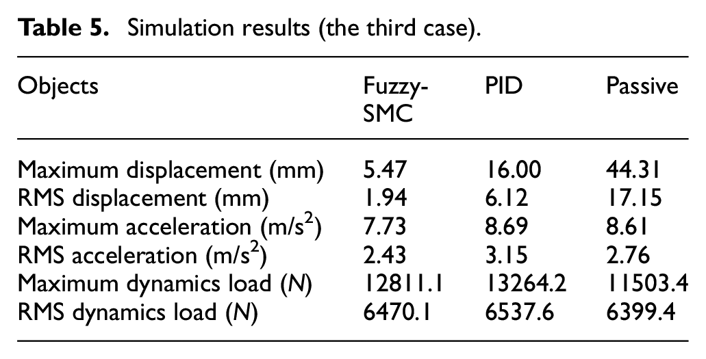
The sprung mass displacement changes continuously according to excitation of the road surface (Figure 13). This is an entirely random variation; it does not follow any rules. The car oscillation is most remarkable when it has only conventional suspension; this value reaches 44.31 mm. These figures can be declined to 16.00 and 5.47 mm if active suspension is used. Compared with the two mentioned cases, the RMS value of displacement, in this case, is relatively small, reaching only 17.15, 6.12, and 1.94 mm. The vehicle body displacement is always guaranteed once the FSMC technique controls active suspension.

Figure 13.

Sprung mass displacement (Case 3).

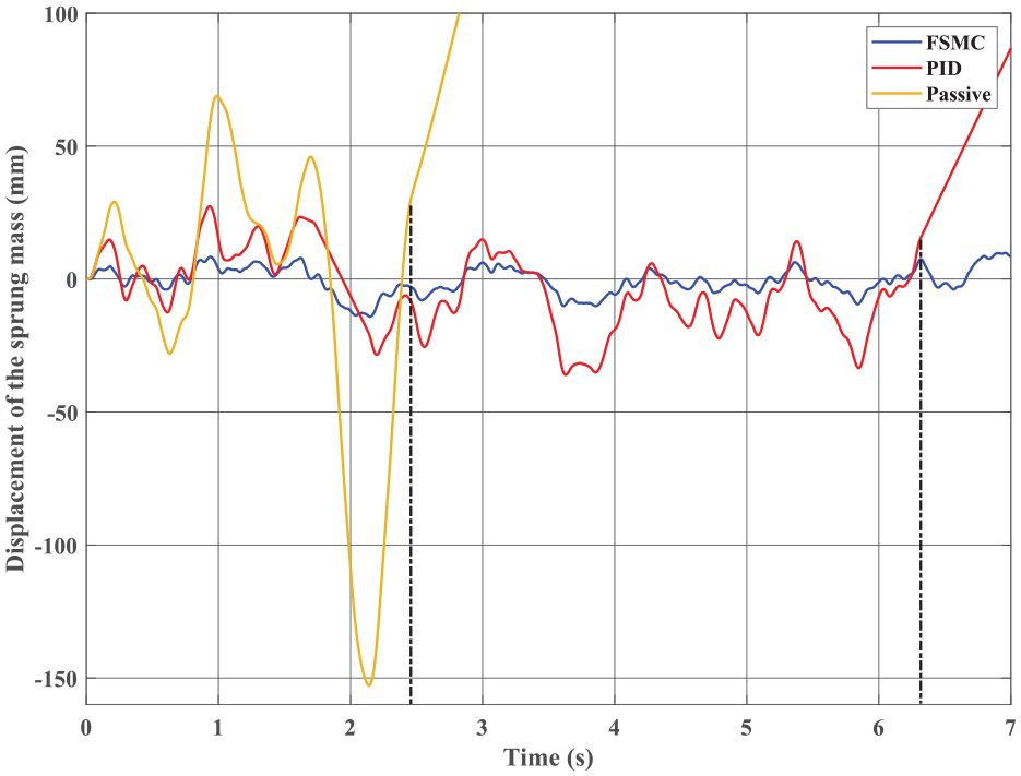
Although the car body displacement is not large, its acceleration is tremendous (Figure 14). Acceleration also varies continuously over time with large amplitude. According to simulation results, if the car does not have an electronic suspension system, the peak acceleration value can be up to 8.61 m/s². If the PID algorithm controls electronic suspension, the peak acceleration value can be slightly larger, reaching 8.69 m/s². Therefore, linear control algorithms (such as PID, etc.) are unsuitable for nonlinear systems. Meanwhile, the body’s acceleration can be reduced to 7.73 m/s² once the FSMC integrated algorithm is used. The smoothness and comfort of the car will still be better when the new technique is applied.

Figure 14.

Sprung mass acceleration (Case 3).

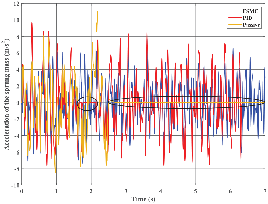
The variation of dynamics load in the third case is much more considerable than in the previous two cases (Figure 15). At some point, the wheel vertical force has reached its limit. The wheel is in danger of being separated from the road surface. However, this problem only lasted for a brief period. Therefore, the stability of the vehicle has not been affected too much. Because active suspension produces a force that acts on both the sprung and unsprung masses at the same time, therefore, the dynamics load variation is also quite significant. It can even be more extensive than in the case of a vehicle using passive suspension. Their RMS values are 6399.4, 6537.6, and 6470.1 N, respectively, for three scenarios: Passive, PID, and FSMC.

Figure 15.

Dynamics load (Case 3).

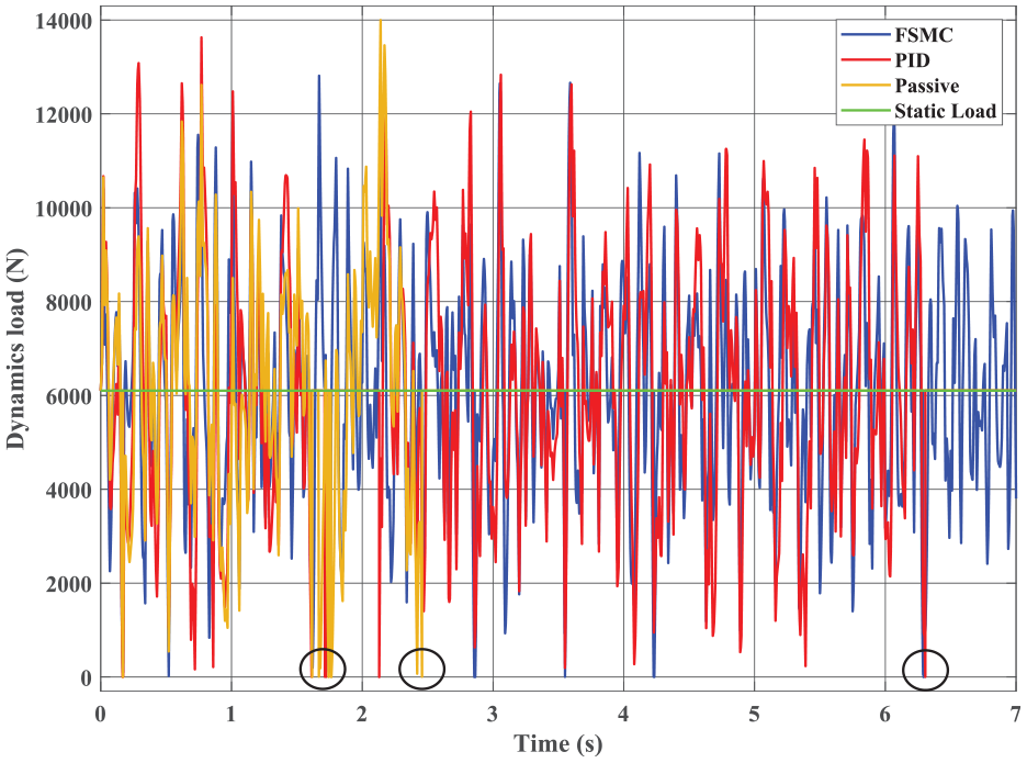
In this case, the study’s findings are illustrated in Table 5.

Table 5.

Simulation results (the third case).

Objects	Fuzzy-SMC	PID	Passive
Maximum displacement (mm)	5.47	16.00	44.31
RMS displacement (mm)	1.94	6.12	17.15
Maximum acceleration (m/s2)	7.73	8.69	8.61
RMS acceleration (m/s2)	2.43	3.15	2.76
Maximum dynamics load (N)	12811.1	13264.2	11503.4
RMS dynamics load (N)	6470.1	6537.6	6399.4

The final case

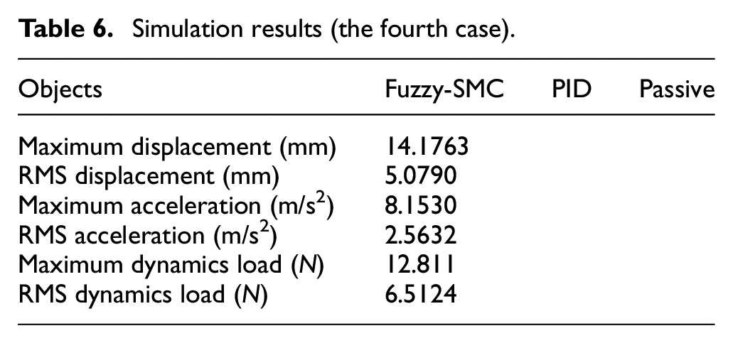
In the last case, the road excitation is the greatest. Both the frequency and amplitude of the stimulus are risen. Therefore, the vehicle oscillation is also more prominent. The simulation results show the wheel is lifted off the road surface at t = 2.4 s if the car only uses mechanical suspension. Even the wheel is detached from the road surface at t = 6.3 s when active suspension controlled by the PID controller is used (Figure 16). When the wheel is separated from the pavement, the acceleration of the vehicle body will decrease to zero, as shown in Figure 17. Besides, the change in the dynamics load will no longer exist (Figure 18). At this point, instability can occur.

Figure 16.

Sprung mass displacement (Case 4).

Figure 17.

Sprung mass acceleration (Case 4).

Figure 18.

Dynamics load (Case 4).

As for active suspension controlled by the FSMC technique, the wheels can still interact with the road well. At some point, the wheel vertical force may approach zero. Nonetheless, it might regenerate instantly. In addition, the figures for vehicle body displacement and acceleration are not excessively high. Consequently, stability and comfort are always assured.

The outcomes of the simulation procedure are outlined in Table 6 (the final case), which may be seen here.

Table 6.

Simulation results (the fourth case).

Objects	Fuzzy-SMC	PID	Passive
Maximum displacement (mm)	14.1763
RMS displacement (mm)	5.0790
Maximum acceleration (m/s2)	8.1530
RMS acceleration (m/s2)	2.5632
Maximum dynamics load (N)	12.811
RMS dynamics load (N)	6.5124

The simulation results obtained from the four cases mentioned above show that: (1) Vehicle body displacement and acceleration increase as the value of the excitation input increases; (2) The most significant change belongs to the Passive situation, while the change of the FSMC situation is not significant; (3) In the first two cases, the change in dynamics load is relatively small. This does not affect road holding; (4) The change in dynamics load is enormous in the last two cases. Regarding the third case, the value of the dynamics load decreases close to zero at some point. As for the last case, the wheels are entirely lifted off the road when the car has only passive or active suspension controlled by the traditional PID algorithm. This is not the case for the FSMC algorithm proposed in this work; (5) The vehicle body acceleration in the last two cases is much larger than the above two cases. This is expressed in both the peak value and the RMS value. In general, sine wave excitation is often used in simulation problems to evaluate the performance of control algorithms. In contrast, random excitation strongly influences moving conditions, which is consistent with reality.

Comparison between FSMC and conventional SMC

A comparison between the results obtained from the FSMC and conventional SMC algorithms is shown in Figures 19 and 20. These results reflect the oscillations of the vehicle body when subjected to sine wave excitation, described in the second case (Figure 6). Looking at Figure 19 more closely, one can see that the vehicle body displacement in the FSMC situation is lower than that of the SMC. This difference is not too significant; however, the vehicle’s smoothness is negatively affected by the chattering phenomenon, which belongs to the SMC situation. This causes small and continuous oscillations in the vehicle body throughout the simulation period.

Figure 19.

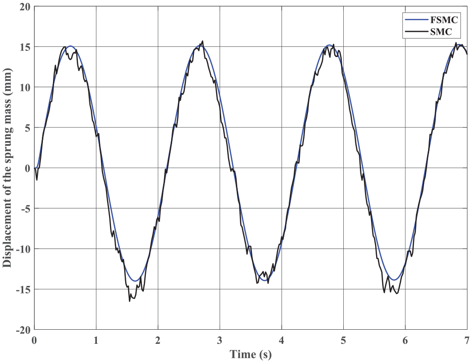
Sprung mass displacement.

Figure 20.

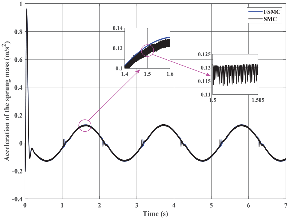
Sprung mass acceleration.

Vehicle body acceleration is also affected by chattering, which is caused by the conventional SMC algorithm. Compared to SMC, the FSMC algorithm provides more outstanding performance in eliminating the effects of chattering (Figure 20). As a result, the vehicle’s ride comfort is significantly improved once the FSMC technique is applied instead of the conventional SMC.

Conclusion

The active suspension system is used to improve vehicle oscillation control. The novel integrated algorithm called FSMC is proposed in this work to improve the performance of the active suspension system under various oscillation conditions. The quality of the proposed algorithm is evaluated through simulation in four cases. According to simulation results, the car body displacement and acceleration value are the smallest in all four cases when the automobile uses active suspension controlled by the FSMC technique. The wheel can be separated from the road in the last case if the classical PID algorithm is used instead of FSMC. This can significantly affect the stability and comfort of the car. Additionally, the phenomenon of “chattering” does not appear when the SMC technique is synthesized with the Fuzzy method.

The numerical simulation process has demonstrated the performance of the FSMC controller. At some point, the value of the acceleration is still significant. This can be solved by integrating a PID algorithm for a single object (vehicle body acceleration). This combined process will be carried out in future research.