
Abstract
Research on initial errors and constraint restrictions is one of the main research directions in the field of control of uncertain robotic systems. An adaptive iterative learning control (AILC) method based on radial basis function (RBF) neural network is proposed to address the trajectory tracking problem of the long-stroke hybrid robot system with random initial errors and full state constraints. The RBF neural network is used to approximate the unknown nonlinear terms, and the network weights are updated using an iterative learning law that incorporates a projection mechanism. Additionally, a robust learning strategy is used to compensate for both the approximation error of the neural network and the external disturbances that vary with each iteration. To relax the requirement of traditional iterative learning control (ILC) for identical initial condition, an equivalent error function is constructed based on the time-varying boundary layer. The tangent-type barrier Lyapunov function (BLF) is designed to ensure that the joint position and speed of the robot system are bounded within a predetermined range. Through stability analysis based on barrier composite energy function (BCEF), it can be proved that the boundedness of all signals in the closed-loop system and the tracking error of the robot system will converge to an adjustable residual set asymptotically. Finally, through simulation experiments conducted on the MATLAB platform, the results demonstrate that the method overcomes the random initial errors of the system effectively, ensures that the system satisfies the full-state constraints, and realizes high-precision trajectory tracking.
Keywords
Introduction
With the development of robotics technology and the arrival of the intelligent manufacturing era, the application demand for robots in modern industry has become increasingly complex. Robots with variable structures have emerged.1,2 A long-stroke hybrid robot is a special structural robot that combines translational and rotational joints, mainly used in the field of high-precision automatic machining and assembly. In actual production processes, robot manipulators are often used on assembly lines to perform tasks such as handling, painting, and injection molding. The action trajectories executed by the robot manipulators are all singular and repetitive.3,4 With increasing of the system operation time and the impact from the external environment, the tracking error will increase gradually, and it will become more difficult to improve the control effect of the system.
Nowadays, the actual working environment of robot systems is becoming more complex, and there are many uncertain factors such as vibration, 5 friction, 6 load variation, 7 random disturbances, and unmodeled dynamics. 8 Those uncertain factors make it impossible to obtain a complete and accurate robot system model. In order to overcome adverse effects from the uncertainty and unknown interference, and also to improve their anti-interference ability, various control strategies have been developed and studied for robot systems, such as adaptive control, 9 fuzzy control,10,11 neural network control,12–14 and sliding mode control.15–17 Adaptive control is suitable for systems with parameter uncertainty and can compensate for parameter uncertainty effectively. Sliding mode control is widely used in uncertain control systems due to its simple design and good robustness, but it often suffers from chattering. At the same time, various approximation tools are often used to address unknown nonlinear problems in systems, such as fuzzy logic system (FLS) and neural network (NN). Therefore, many scholars have combined these approximation tools with adaptive control to design controllers. Jiang et al. 18 employed a radial basis function neural network (RBFNN) to cope with inevitable dynamic uncertainties and utilized a new composite learning law to update the weights of the neural network. Sun et al. 19 used an adaptive NN method to approximate the unknown nonlinearity, while using a tangent-type BLF to satisfy the constraint. Ruan et al. 20 used the error transformation method to convert constrained system variables into unconstrained variables, used the FLS to approximate the unknown nonlinear terms, and designed a fault-tolerant control scheme to ensure that the system satisfies the constraints. Overall, trajectory tracking control of uncertain robot systems remains a meaningful fundamental control problem.
Generally, when a robot system performs repetitive tasks, the reference trajectory is consistent within a fixed operating time. However, with the time increasing of system operation, the tracking error increases gradually. Iterative learning control (ILC) is an intelligent control method that can reduce the system error gradually during each operation, and can also improve the system tracking performance with the increasing of operation number. Therefore, the ILC strategy is a suitable choice for application in such robot systems. It is the core design idea of the ILC method that update and optimize the controller constantly during each iteration. The previous control input information and trajectory tracking error are used in the current controller to adjust and modify the controller, reduce the tracking error gradually, and achieve the expected trajectory tracking of the controlled object. The primary objectives of utilizing contraction mappings in traditional ILC theory are to enhance the stability, convergence, and robustness, and reduce oscillations of the control system. As the requirements for the control accuracy and speed of robot systems increase gradually, the traditional ILC method can no longer meet the application requirements. In recent years, some scholars have applied Lyapunov-like function theory to the design of ILC and proposed adaptive iterative learning control (AILC). AILC not only possesses the characteristics of improving control performance gradually found in traditional ILC but also incorporates the advantages of adaptive control. Liu et al. 21 used an adaptive controller to compensate for the uncertain parameters in the system and used a feedback ILC method to estimate the external disturbances. Bensidhoum and Bouakrif 22 designed an AILC scheme to address the problem of reduced stability in a robot system caused by varying disturbances and input dead zones. They used an adaptive iterative control law to estimate the optimal weights of the RBFNN. The AILC algorithms proposed above assume that the control object satisfies perfect reset condition. However, in engineering application, the actual mechanical structure will limit the accuracy of the physical resetting. When there is an initial bias, it is extremely challenging for a robot system to ensure that the system state remains strictly on the desired trajectory every time it executes a repetitive task. The existence of non-zero initial errors prevents the system from satisfying the requirement of having identical initial conditions in ILC. This requirement of identical initial condition has restricted the further development of ILC. Overcoming the impact of initial errors on the system has become a research focus for scholars both domestically and internationally. The existing methods for overcoming the effect of initial errors include initial rectification, 23 time-varying boundary layers,24,25 and error tracking strategies.26,27 Zhang et al. 23 constructed an initial rectification auxiliary reference signal to overcome obstacles caused by non-zero initial errors during ILC design. Chien et al. 24 first proposed the method of time-varying boundary layers, and Guan et al. 25 overcame the difficulty of non-zero initial errors of a pneumatic artificial muscle drive mechanism. Yan et al. 26 constructed an expected error trajectory and designed a controller to drive the actual system error to track the constructed expected error trajectory gradually, thereby breaking through the requirement of the traditional ILC algorithm that the initial error must be zero. Hong et al. 27 dealt with the random initial position of a tank gun system by using the error tracking strategy, and approximated the unknown nonparametric uncertainties of the tank gun system by using a FLS. Hence, further research is required to explore more effective and efficient methods for addressing the initial state problem in uncertain robot systems that perform repetitive tasks.
In practical application of robot system, due to the influence of the working environment and hardware performance, robots are limited by various conditions during operation, such as input constraints, 28 output constraints,29,30 and state constraints.31,32 Failure to comply with these constraints may result in a decline in control performance, potential hardware damage, and even endanger the personal safety of operators. Hence, it is essential to take these constraints into account when designing controllers for robot systems. In recent years, an analysis method known as the barrier Lyapunov function (BLF) has been developed, and the barrier function is often employed to ensure that the objective function remains within the predetermined region consistently, thereby achieving the goal of constraining the objective variable. Yu et al. 33 introduced a composite energy function 34 for theoretical proof, demonstrating that the proposed AILC algorithm can confine system states and inputs within predefined limits. Min et al. 35 designed a backstepping control method based on RBFNN and BLF, and Cruz-Ortiz et al. 36 proposed a BLF for stability analysis of the designed robust finite time controller. Both their methods ensure that the system meets the full state constraints. During industrial production, the actual state variables change with time, and the time-varying restriction can be more complex and general than the previously mentioned restriction problems. To address the time-varying restriction in the robot system, Lu et al. 37 used a time-varying BLF to ensure that the system state remains within a predetermined time-varying range. From the above analysis, research on achieving improved and faster control performance is a central focus of robotic control systems under constraints that ensure system safety.
So far, many scholars have conducted research on uncertain robotic systems with initial errors or constraint limitations. However, in the field of robotic control, there still exists a gap in research addressing uncertainty, random initial errors, and constraint limitations simultaneously. On the one hand, the practical working environment of long-stroke hybrid robots is complex, and the changing heavy loads may cause unpredictable deformations in the robotic manipulator. At the same time, there are uncertain factors such as vibration, friction, and unmodeled dynamics, which can also affect the accuracy of robotic manipulator reset, leading to a decrease in the stability of the long-stroke hybrid robot system. On the other hand, considering the safety and motion range restrictions during the operation of long-stroke hybrid robots, the positions and speeds of each joint of the robotic manipulator must be limited within specified boundaries. To address the issue of poor robustness in systems with both system uncertainty and random initial errors, and where the system needs to satisfy full-state constraints, this paper proposes a robust iterative control algorithm based on adaptive learning neural networks for long-stroke hybrid robot under full state constraints. The main contributions of this paper are as follows:
(1) In response to system uncertainty and random external disturbances, an RBF neural network is used to approximate unknown nonlinear terms in uncertain robot systems. A robust term is designed to compensate for the approximation error of the neural network and random external disturbances. The network weights and the unknown upper bound of both the approximation error and random external disturbances are continuously updated according to the projection iterative learning law.
(2) To address the non-zero and random initial errors of uncertain robot systems in each iteration, a time-varying boundary layer is constructed to counteract the random expansion error at the initial time. An equivalent error function is designed with an initial value of zero, and this equivalent error function is utilized as the main control variable for the iterative controller to relax identical initial conditions.
(3) To address the simultaneous existence of system uncertainty and random initial errors, while also ensuring the system satisfies full-state constraints, a tangent-type BLF is introduced in the design of the robust iterative control algorithm. This BLF constrains the system states within predefined bounds, allowing for high-precision and robust trajectory tracking while ensuring the safe operation of the robotic system.
The rest of this paper is organized as follows: In Section “System description and preliminaries”, a dynamic model of the long-stroke hybrid robot system is established, the system is transformed, and basic assumptions are provided. In Section “Controller design and stability analysis”, an AILC scheme based on the RBF neural network is designed, a barrier composite energy function is constructed, and stability analysis is conducted on the robot system. In Section “Simulation results”, simulation experiments based on the MATLAB platform are presented. This paper is summarized in Section “Conclusion”.
System description and preliminaries
Robot system dynamics
A long-stroke hybrid robot is composed of a combination of translational and rotational joints, and Figure 1 shows its structural schematic diagram. We define the base coordinate system
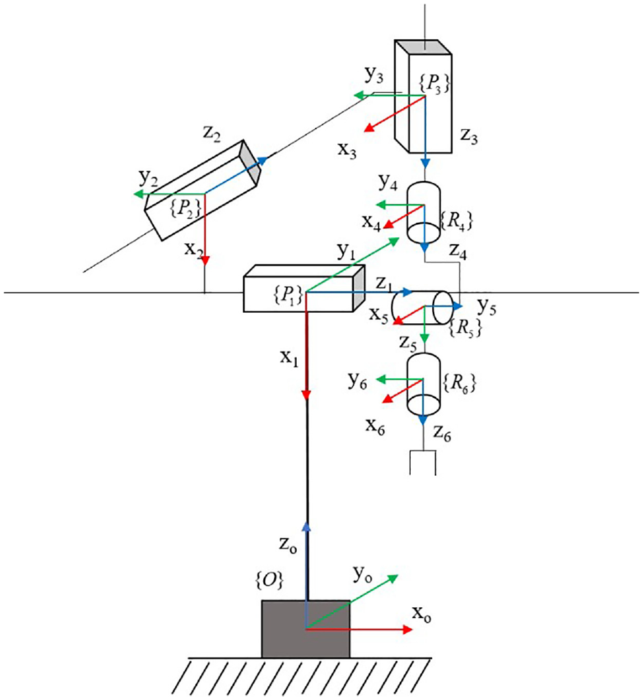
Structure diagram of the long-stroke hybrid robot.
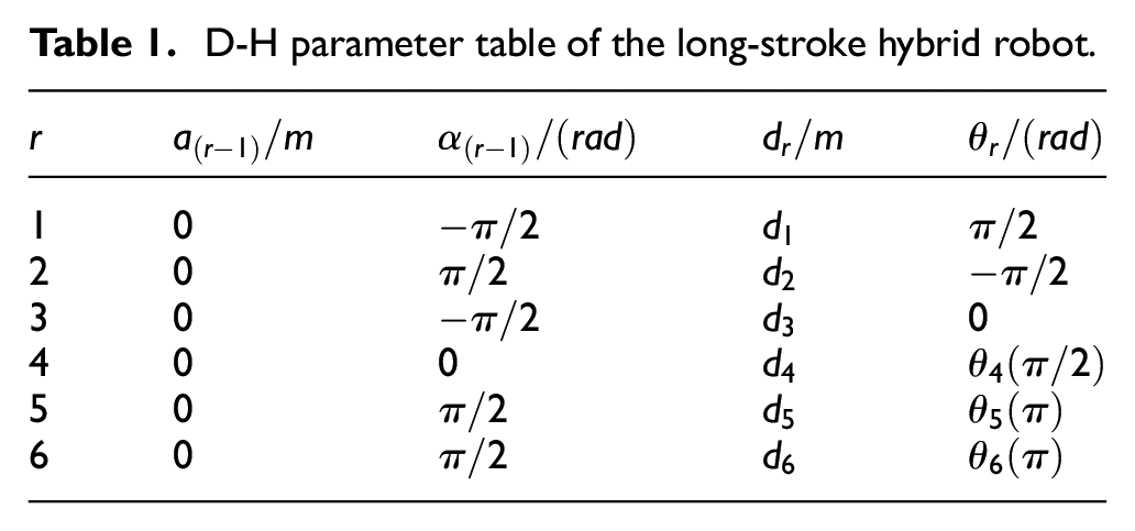
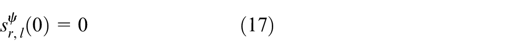
As shown in Table 1, after determining these coordinate systems, we can obtain the D-H parameter table of the long-stroke hybrid robot.
D-H parameter table of the long-stroke hybrid robot.
To facilitate the analysis and experimental comparison, we analyze and study a long-stroke hybrid robot composed of three-axis translational joints and three-axis rotational joints. The moving base, consisting of translational joints, and the multi-axis mechanical manipulator with rotational joints are treated as two subsystems. Considering the interaction forces between the rigid manipulators, their dynamic equations are expressed as:


Equation (1) describes a moving base subsystem composed of translational joints, and equation (2) describes a robot manipulator subsystem composed of rotational joints.
where
This paper primarily focuses on the subsystem of the rotating-joint robot manipulator of the long-stroke hybrid robot. To ensure the universality of the conclusions in this paper, a rotating-joint robot manipulator with n-DOF is considered to operate repeatedly in

where
For simplicity, the time-independent variable
System transformation and basic assumptions
We define
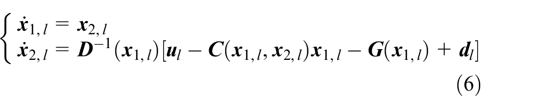
Equation (6) can be expanded to:
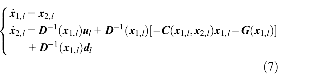
In this equation,
The RBF neural network possesses excellent generalization ability and a simple network structure, consisting of three layers: input layer, hidden layer, and output layer. The neurons in the hidden layer of RBF neural network use activation functions, which have nonlinear mapping ability. This mapping enables the RBF neural network to approximate any nonlinear function within a compact set and with any accuracy. Consequently, in control system design, RBF neural networks are often used as function approximators for unknown functions. When integrating the RBF neural network into the controller, relying on the self-learning ability of the neural network, the neural network controller can improve the control performance of the uncertain systems and achieve the desired tracking accuracy.38,39 The adaptive and learning capabilities of neural networks make them suitable for handling complex and uncertain control tasks.
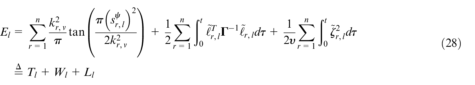
The output
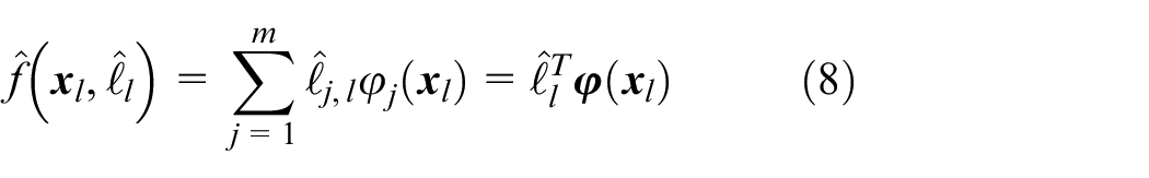
where
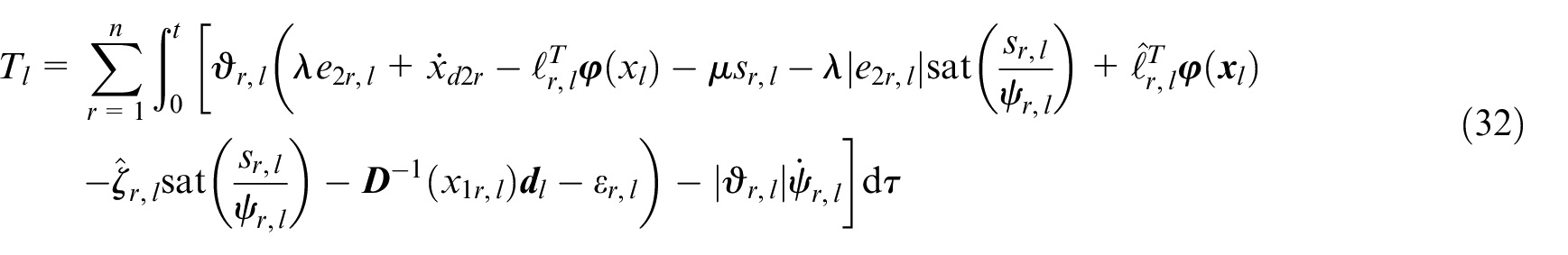
There exists an optimal set of neural network weights

The approximation error
where
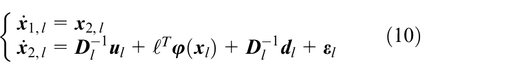
For the rotating-joint manipulator subsystem described in (5), this paper designs an adaptive iterative learning controller
Controller design and stability analysis
Design of an iterative learning controller based on the RBF neural network
First, we define the state tracking error
Then, we can define the extension error

where
If
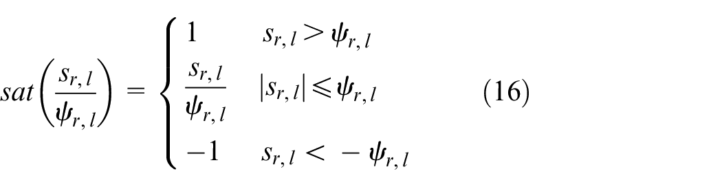
The following equation holds for the design of time-varying boundary layer


where
From equation (13), it can be inferred that the value of time-varying function
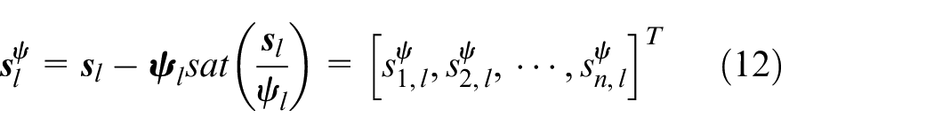
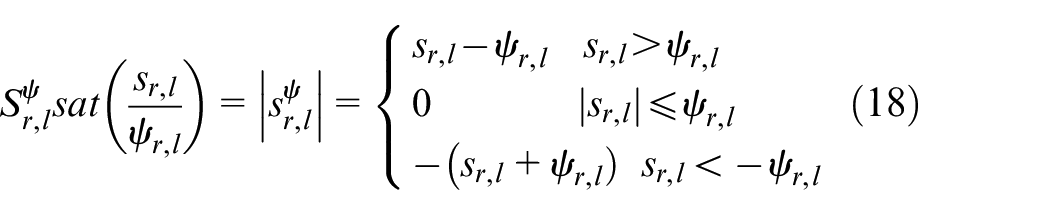
In equation (12),
To facilitate stability and convergence analysis, the following properties of
According to the variables defined above, the controller
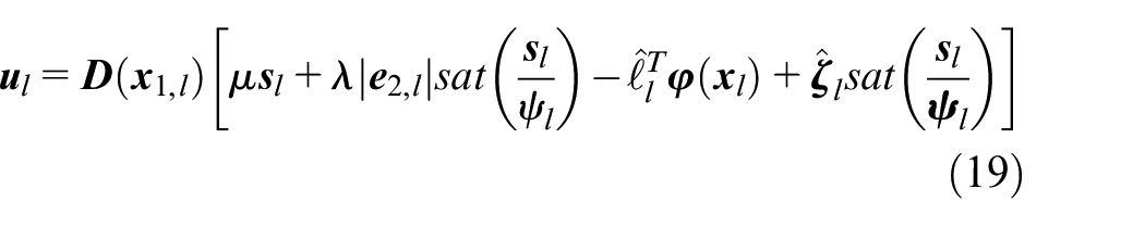
where
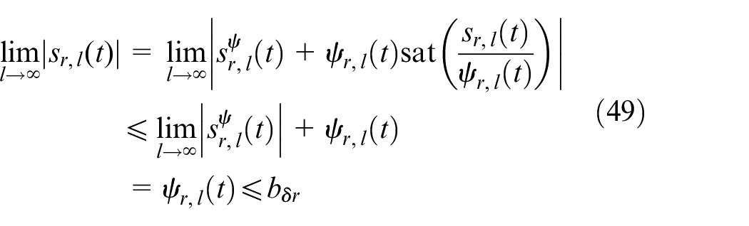
For unknown neural network weights
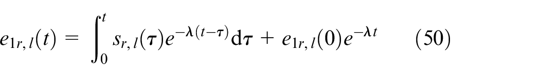
where
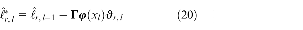
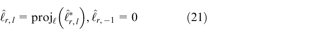
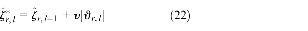
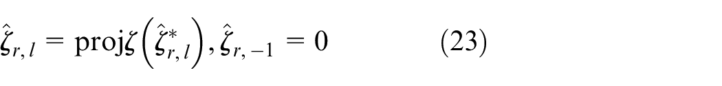
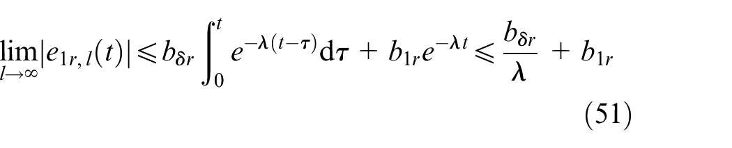
To ensure that the estimated values of the parameters are always within the appropriate range, a projection mechanism is introduced as follows:
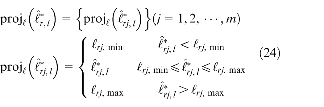
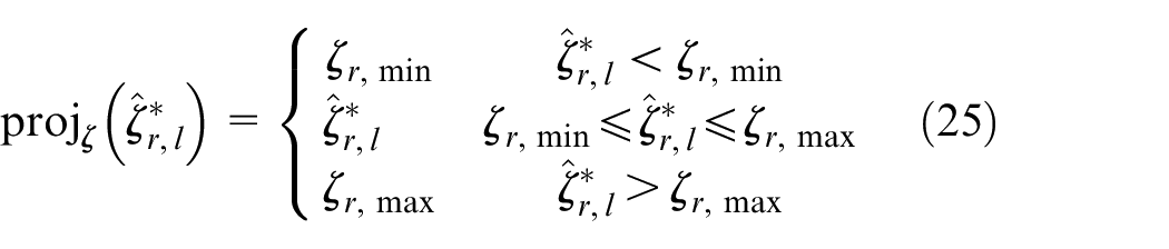
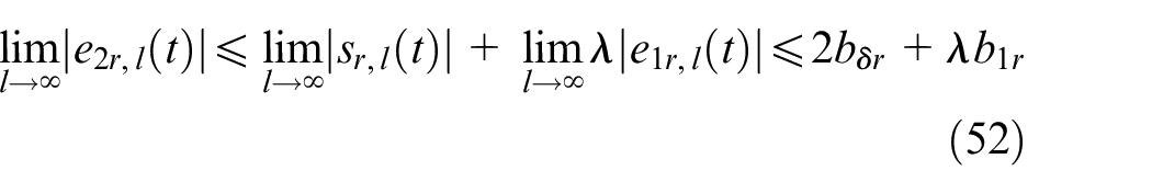
where
The robot system diagram using the proposed method is shown in Figure 2. In the diagram, the feedback term, neural network approximation term, and robust compensation term together constitute the proposed AILC (18). The parameter learning law is implemented by (20)–(23).
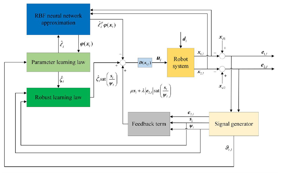
Block diagram of robot system using the proposed method.
Stability analysis
For the convenience of analysis and proof, the lemma that will be used in this paper is given below.


The theoretical summary of the system is shown in Theorem 1.
where
The proof of Theorem (T1) is as follows:
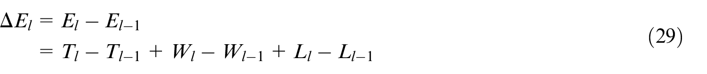
We will prove Theorem (T1) in three steps. The first step proves the negative definition of the BCEF, the second step proves the boundedness of the BCEF, and the third step proves the boundedness and convergence of
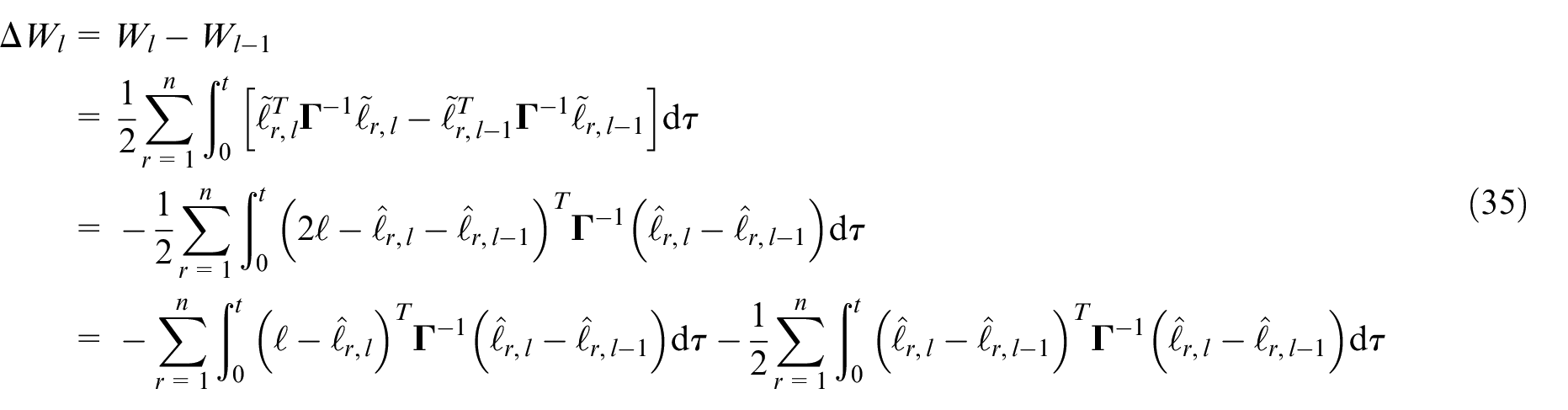
Considering a difference in
According to equations (11) and (12),
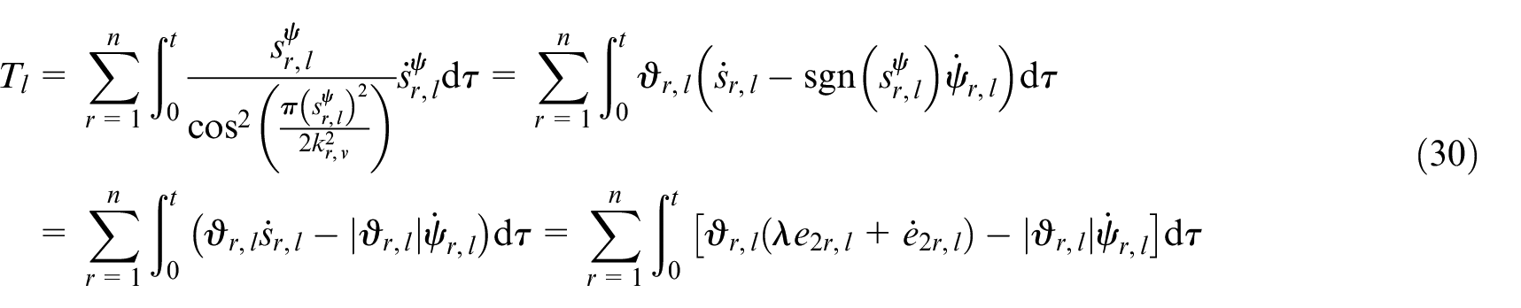
Using the system model (10), equation (30) can be simplified as:
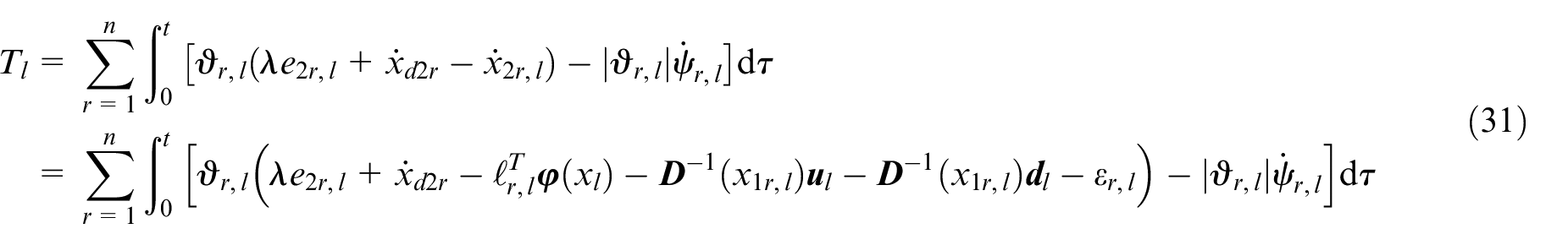
Substituting the control law (19) into equation (31), we obtain:
Since
Since
Considering a difference in
According to the parameter learning laws (20) and (21), equation (35) can be simplified as:
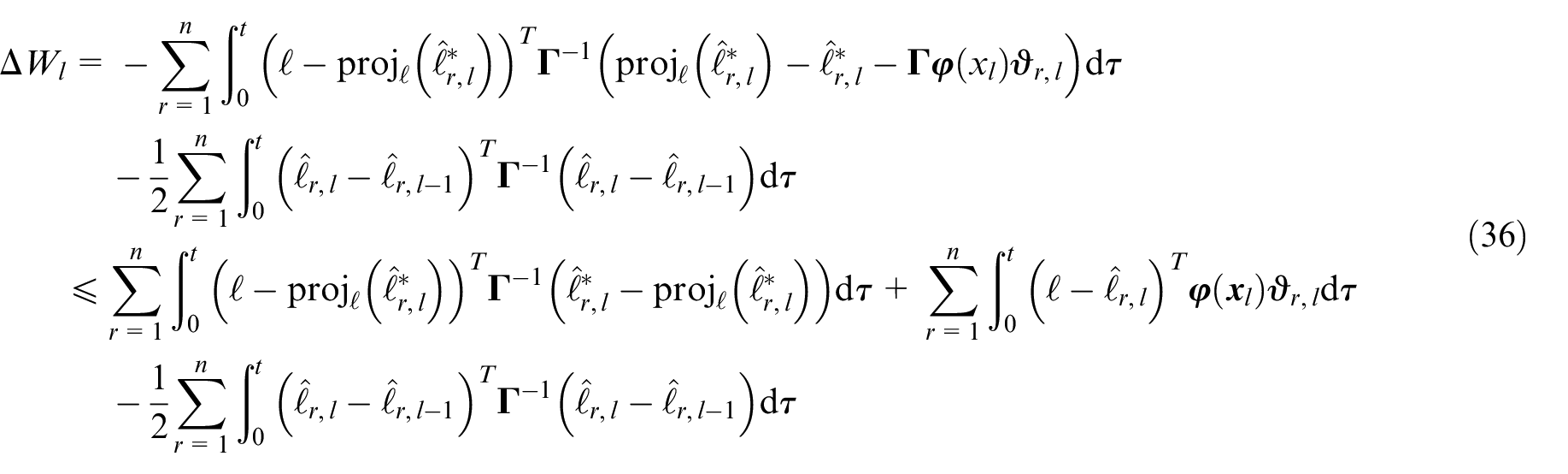
According to equation (26) in Lemma 1, equation (36) can be simplified as:

Considering a difference in
According to the parameter learning laws (22) and (23), equation (38) can be simplified as:
According to equation (27) in Lemma 1, equation (39) can be simplified as:
Substituting equations (34), (37), and (40) into equation (29) yields:
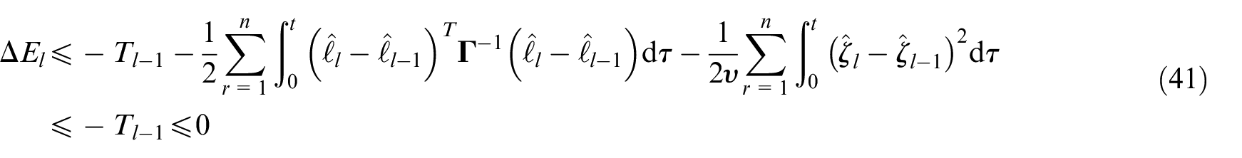
Adding equation (41) from 1 to
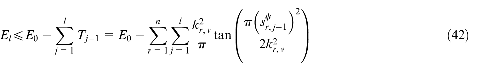
When the number of iterations is infinite, namely,
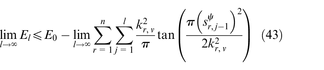
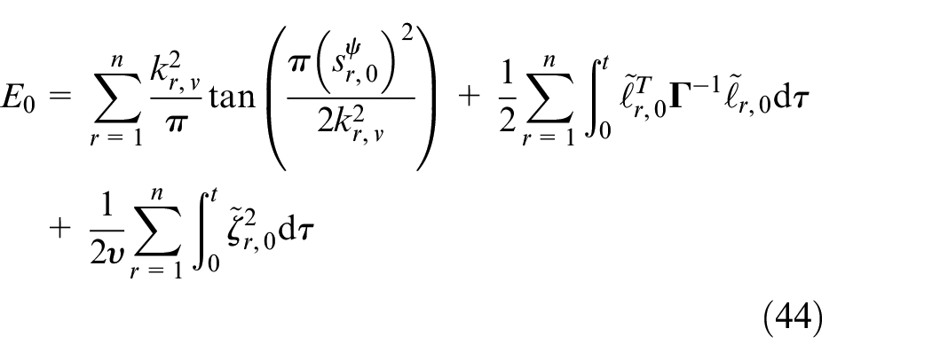
According to equation (41),
When
According to equation (44), the derivative of
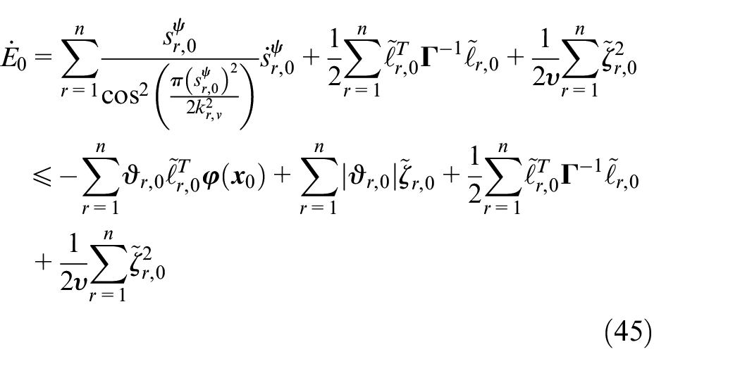
Based on equations (20), (21), (22), and (23), equation (45) can be simplified as:
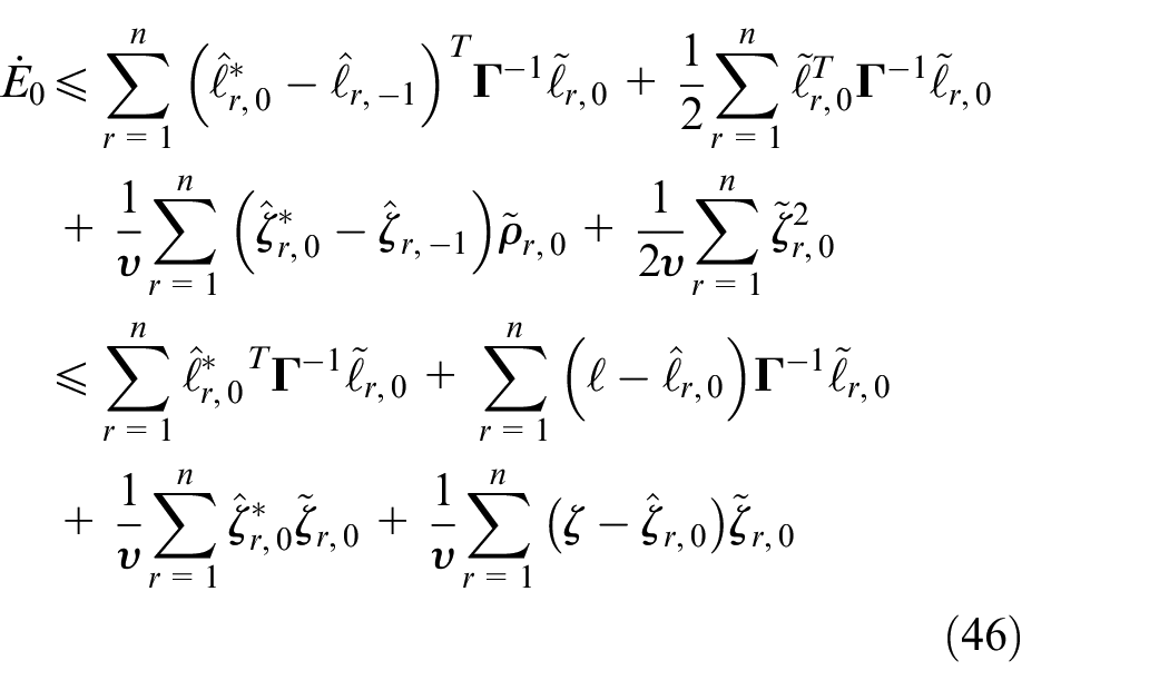
By using equations (26) and (27) in Lemma 1, equation (46) can be simplified as:
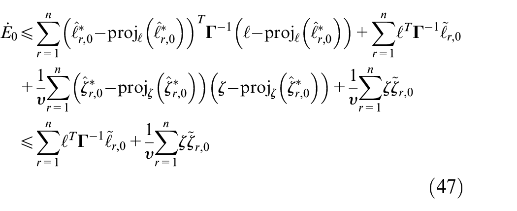
Using Young’s inequality for products, equation (47) can be simplified as:
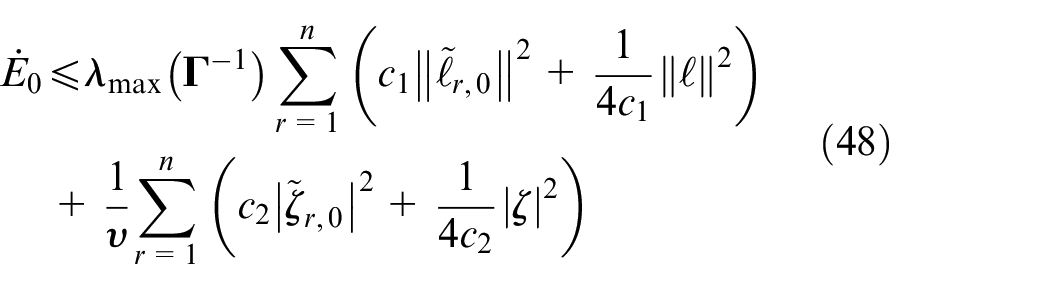
where
According to Lemma 1, both
According to equation (43), since
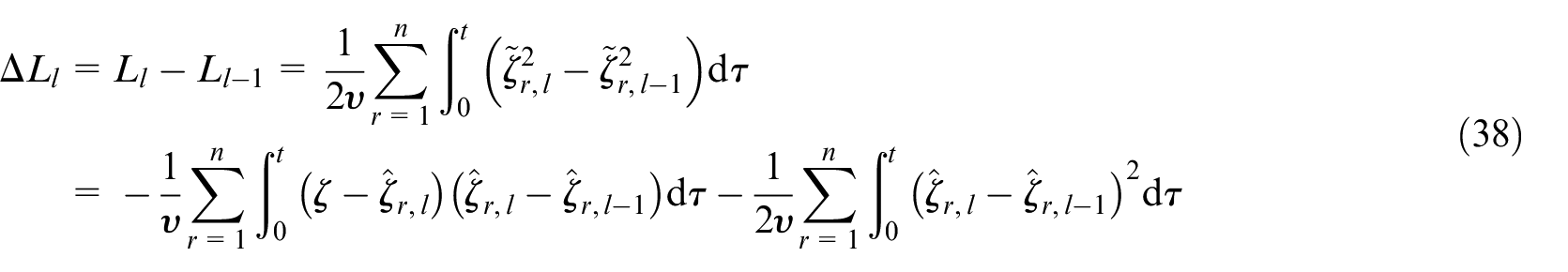
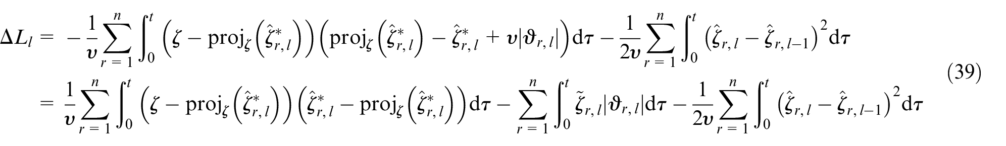
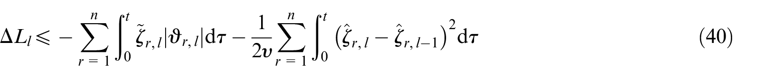
The proof of Theorem (T2) is as follows:
Based on equations (13) and (15),
The proof of Theorem (T3) is as follows:
According to equation (11), we can obtain
Combining Theorem (T2) and Assumption 2, the following can be concluded:
The proof of Theorem (T4) is as follows:
When
Similar to the derivation process of Theorem (T3), it can be obtained that

The above is the entire proof process.
Simulation results
In this paper, an AILC method based on RBF neural network is proposed for the rotating joint subsystem of the long-stroke hybrid robot. To verify the effectiveness of the proposed algorithm, a 2-DOF rotating joint robotic manipulator is used as the validation model for the algorithm. The structural parameters of the model are
where
The mathematical model of the robot system mentioned above is used for simulation verification in MATLAB, and the effectiveness of the controller is analyzed. This simulation is conducted on a personal computer running the Windows 10 operating system with an Intel i5 processor, using MATLAB R2020a software. We use fourth-order Runge-Kutta equation solving in the simulation, with a sampling time of 1 ms. The simulation time is 8 s. The controller and parameter learning laws proposed in this paper are shown in equations (19)–(23). The parameter settings are
The expected position trajectory is
where
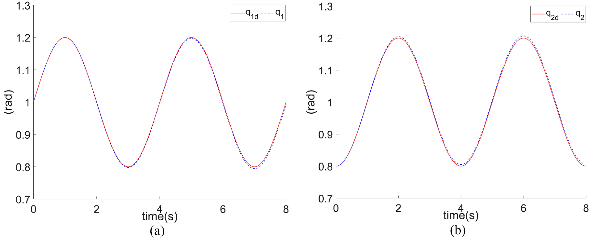
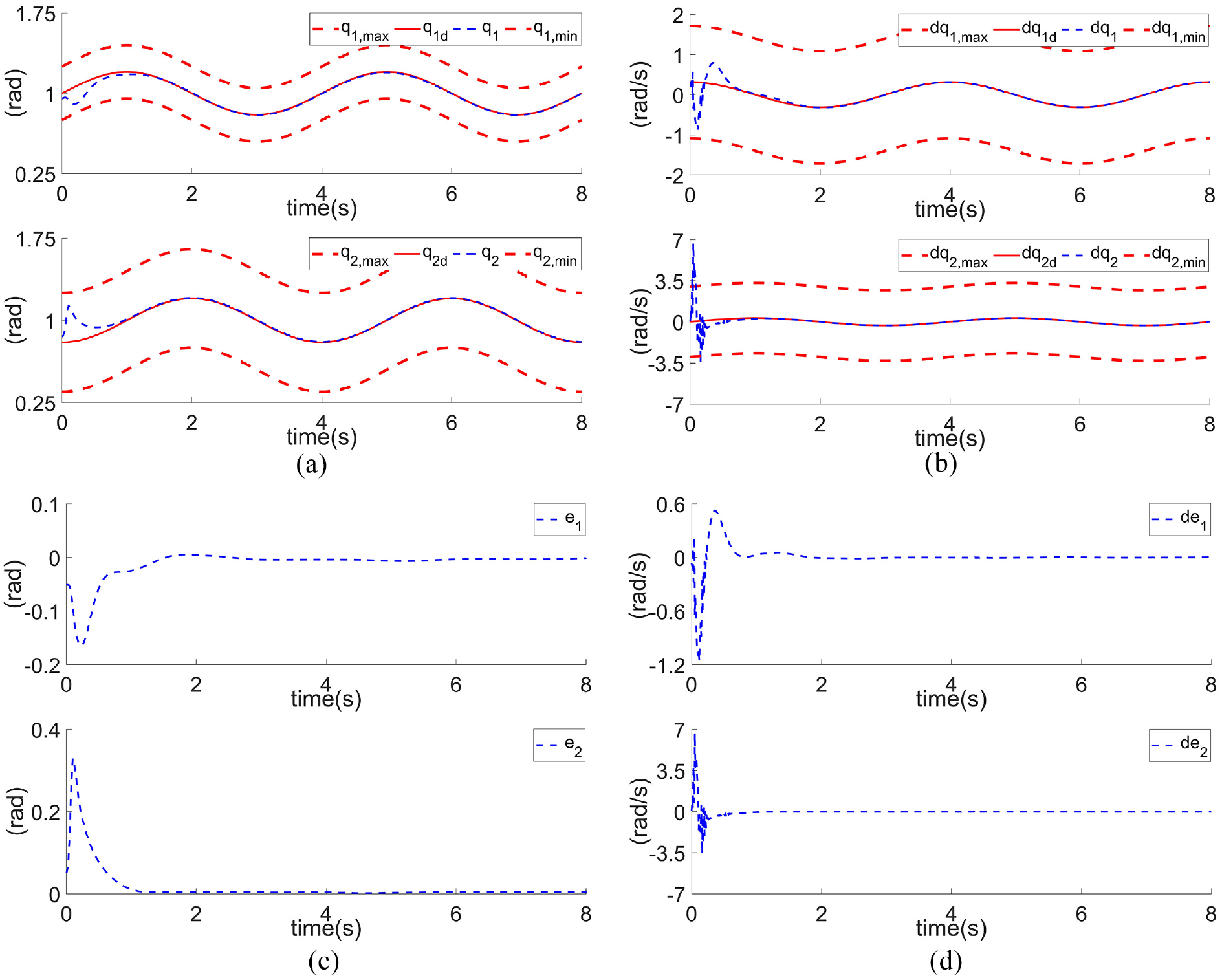
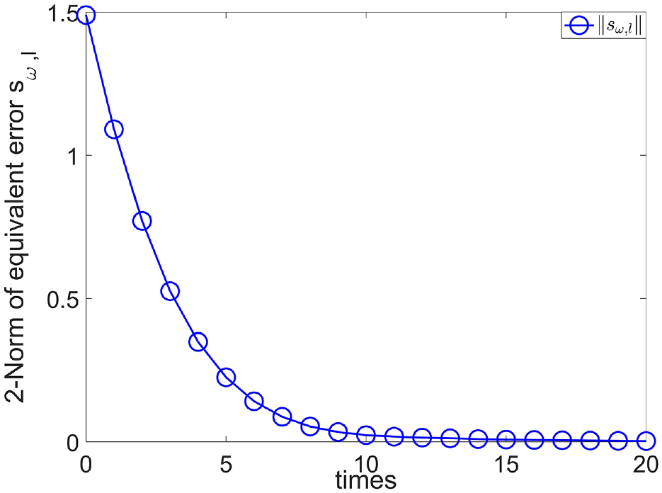
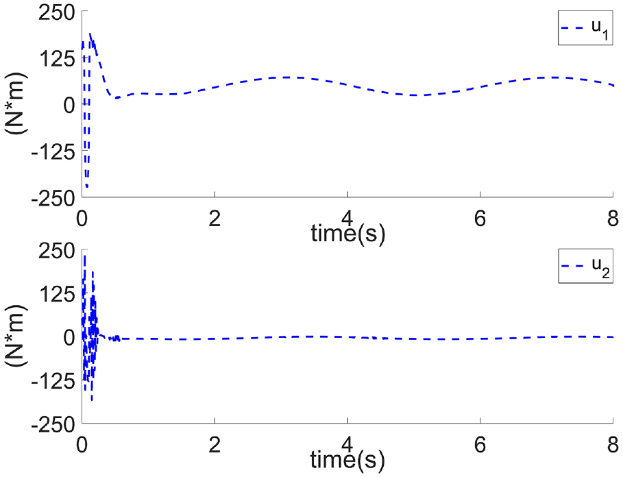
Figures 3 to 5 show the trajectory tracking results of system after 20 iterations. The Figure 3(a) to (d) respectively represent the position, speed tracking curves, and tracking error curves of the two joints. The result of Figure 3 indicates that even with non-zero initial errors, the robot system states track their expected trajectory successfully. From the results of Figure 3(a) and (b), we can see that both the position and speed variables remain within the predetermined range, satisfying the constraint restrictions. Figure 4 shows the learning convergence curve of the equivalent error function of the system, which gradually converges to zero with increasing iterations. Figure 5 shows the system control inputs, and overall, the control inputs are relatively smooth.
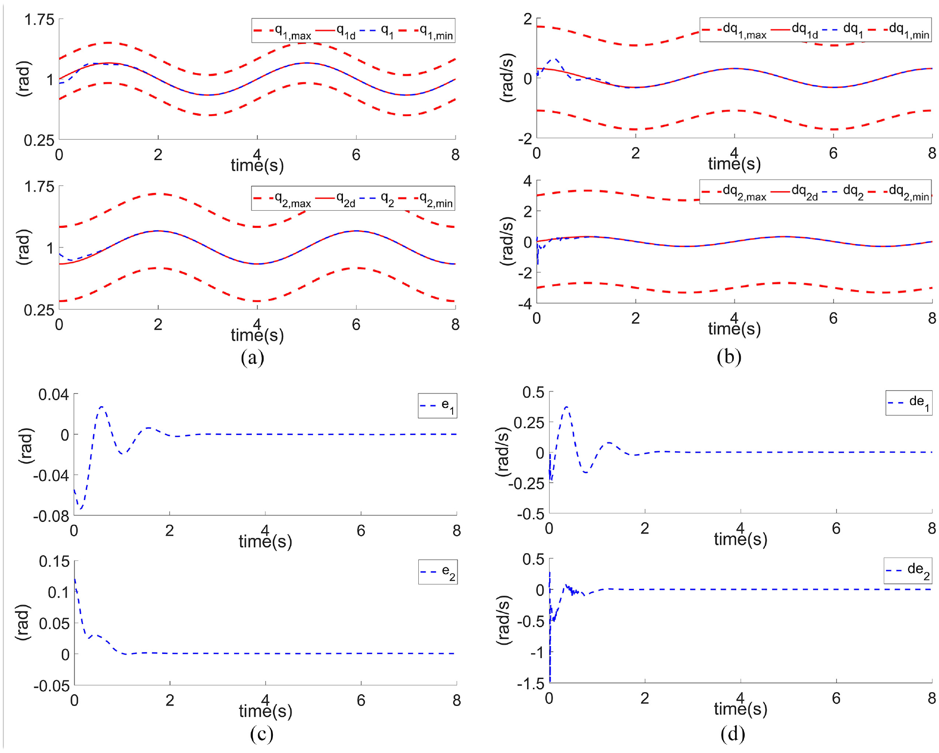
System tracking curve: (a) joint position tracking, (b) joint speed tracking, (c) joint position tracking error, and (d) ioint speed tracking error.
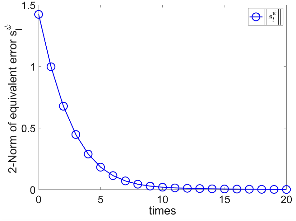
Convergence curve of
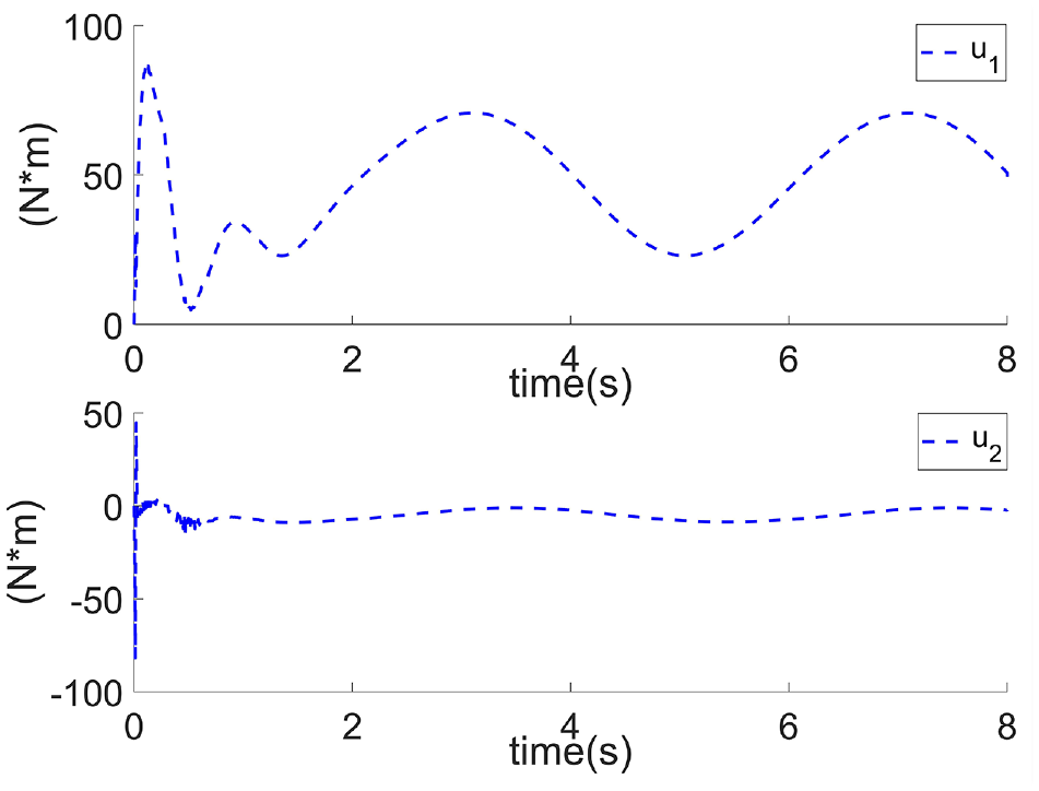
Control input.
We use two comparative experiments to verify the progressiveness of the proposed algorithm.
Comparative experiment 1
The experiment utilizes the AILC scheme proposed by Tayebi. 40 Notably, the impact of non-zero initial errors on the robot system has not been effectively overcame by the controller in this scheme.
The experimental simulation equipment and platform are consistent with the experimental requirements of the proposed method. The expected trajectory and interference term of the system are also the same as in the previous experiment.
Figure 6 shows the position trajectory tracking under zero initial errors condition, while Figure 7 shows the position trajectory tracking under non-zero initial errors condition, respectively. Comparing Figures 6 and 7, non-zero initial errors have a significant impact on the control effectiveness of the system. When there is non-zero initial errors in the robot system, even after adjusting the controller parameters, the system state consistently fails to track the desired trajectory. Consequently, this AILC method is not effective in addressing the trajectory tracking problem in robot systems with non-zero initial errors.
Position trajectory tracking under zero initial errors: (a) joint 1 position tracking and (b) joint 2 position tracking.
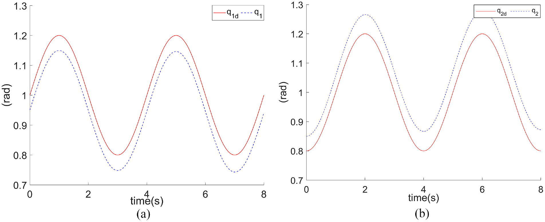
Position trajectory tracking under non-zero initial errors: (a) joint 1 position tracking and (b) joint 2 position tracking.
Comparative Experiment 2
The simulation employs the AILC scheme with initial rectification.41,42 The difference from the method proposed is the use of an initial correction strategy to relax the identical initial condition of robotic system. Despite this modification, the algorithm still employs the RBF neural network to approximate unknown nonlinear terms in the system.
The experimental simulation equipment and platform are consistent with the experimental requirements of the method proposed, and the parameter settings of the RBF neural network and parameter learning laws remain consistent with the aforementioned experiment.
Figures 8 to 10 show the trajectory tracking results of system after 20 iterations. The Figure 8(a) to (d) represent the position, speed tracking curves, and tracking error curves of the two joints, respectively. Figure 8 demonstrates that the initial rectification strategy addresses the problem of initial errors effectively, and the system states can track their expected trajectory ultimately. Figure 9 shows the convergence curve of the corresponding equivalent error function, which eventually converges to zero as the number of iterations increases. Figure 10 shows the control input of system, which undergoes significant changes during the initial period and may cause damage to the robot system.
System tracking curve (Comparative Experiment 2): (a) joint position tracking, (b) joint speed tracking, (c) joint position tracking error, and (d) joint speed tracking error.
Convergence curve of
Control input (Comparative Experiment 2).
Figure 11 shows the tracking performance of the system using the proposed method and the initial correction method used in comparative experiment 2. As shown in Figure 11, after 20 iterations, both control methods successfully drive the system state to track the required trajectory within the allowed error range. It can be concluded that compared to the initial correction method, the proposed method in this paper can track the desired trajectory in a shorter time and with higher tracking accuracy. For joint 1 position and speed tracking, the method proposed in this paper can converge the tracking error in 2.24 s and 1.57 s, shorten the convergence time by 4 s and 3 s, respectively, and achieve tracking accuracy of 10−4 and 4 × 10⁻⁴. For joint 2 position and speed tracking, the method proposed in this paper can converge the tracking error in 2.66s and 1.96s, shorten the convergence time by 2.3s and 3s respectively, and achieve a tracking accuracy of 3 × 10⁻⁵ and 2 × 10⁻⁴. More importantly, the method proposed in this paper ensures that the system state remains within the constraint range. However, as shown in Figure 11(b), under the control of the initial correction method, the joint speed exceeded the constraint range. Figure 12 shows the system control input using the method proposed in this paper and the initial correction method. It can be seen that the control input of the method proposed in this article is smoother and has less jitter in the initial stage.
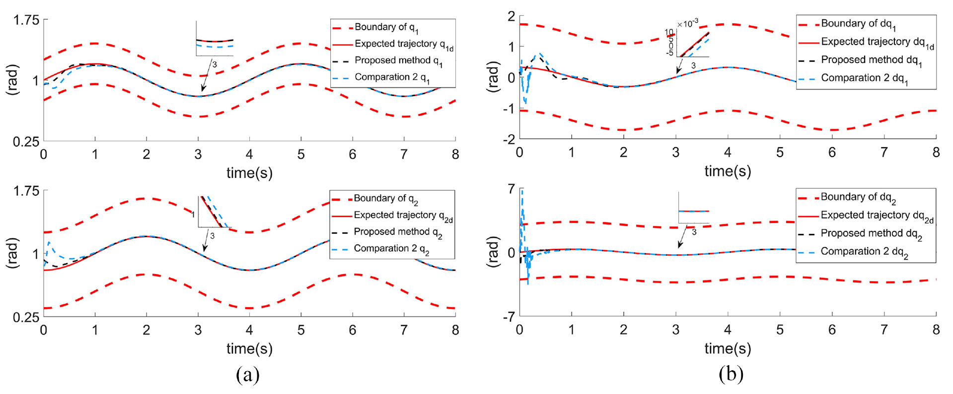
System tracking performance under two comparative methods: (a) joint position tracking and (b) joint speed tracking.
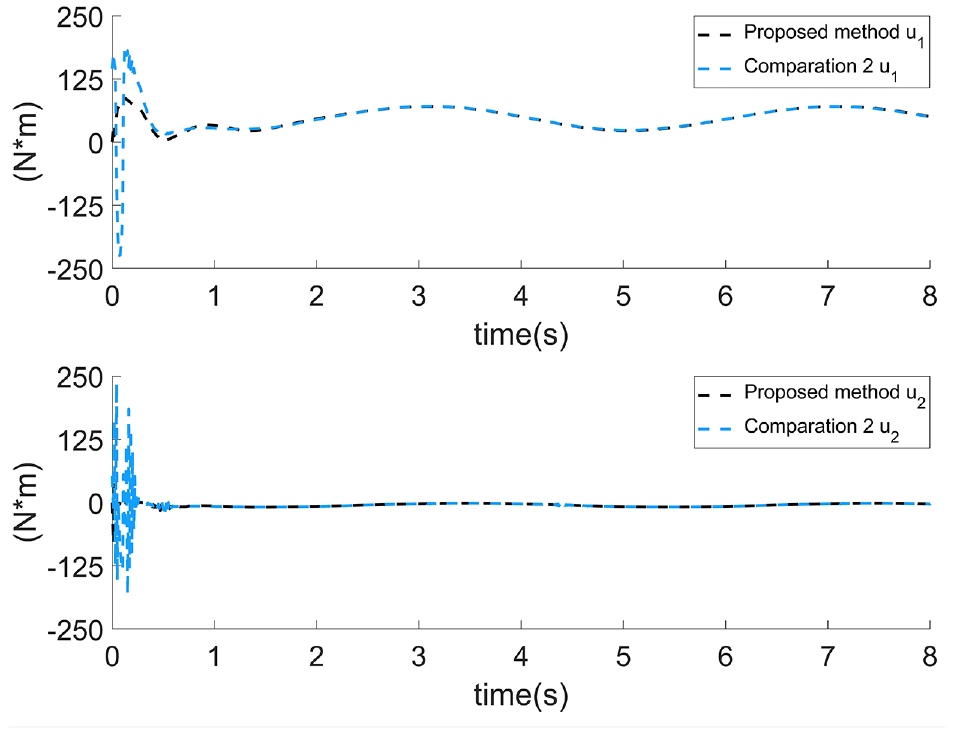
System control input under two comparative methods.
Although both the initial rectification strategy and the time-varying boundary layer can relax the identical initial condition, the design of the time-varying boundary layer is simpler. Therefore, we introduce the time-varying boundary layer to solve the problem of random initial errors.
The results of the above simulation experiments verify the effectiveness of the method proposed.
Conclusion
For the trajectory tracking problem of the long-stroke hybrid robot with initial errors and full state constraints, an AILC method based on RBF neural network is proposed. The adaptive learning neural network is designed to approximate the unknown nonlinear terms in the robot system, and the robust learning method is adopted to compensate for both the approximation error and external interference. An equivalent error function is designed by introducing the time-varying boundary layer to address non-zero random initial errors. The tangent-type BLF is constructed to prevent the system from violating the full state constraints. Through stability analysis based on the BCEF, the proposed control strategy ensures that the system tracking error remains within a very small range, and all signals of the robot system are bounded. Finally, the feasibility of the proposed method is verified by simulation examples on the MATLAB platform. The results of these experiments highlight the significance of overcoming the initial errors and satisfying the constraints of the robotic system. At present, the algorithm has only been simulated numerically using MATLAB. In the future, we plan to establish a real long-stroke hybrid robot experimental platform to verify the effectiveness of the algorithm and make further improvements.
Footnotes
Declaration of conflicting interests
The author(s) declared no potential conflicts of interest with respect to the research, authorship, and/or publication of this article.
Funding
The author(s) disclosed receipt of the following financial support for the research, authorship, and/or publication of this article: This work is partially supported by National Natural Science Foundation of China (No.U1804147), Science and Technology Innovation Talents in Universities of Henan Province(20IRTSTHN019), Henan Provincial Science and Technology Research Project (No.212102210508).
Data availability statement
Data sharing not applicable to this article as no datasets were generated or analyzed during the current study.