High-resolution acoustic imaging method based on equivalent source method and reweighted l 1 minimization

Abstract

Sparse regularization has been successfully applied to equivalent source method (ESM) in order to improve the acoustic imaging resolution. However, the application is not always feasible, especially at low frequencies. To overcome the problem, this paper proposes a high-resolution acoustic imaging method. In this method, reweighted l₁ minimization is introduced to ESM to deal with the ill-posed inverse problems. Then the obtained equivalent source strengths are used to locate the sound sources. Compared to the sparse regularization-based ESM, the proposed method can provide a low side lobe and higher spatial resolution of acoustic imaging. Meanwhile, by arranging equivalent sources in three-dimensional space, the proposed method can also realize the acoustic imaging in three-dimensional sound field with high resolution. The results of the simulation and experiment demonstrate the validations.

Introduction

Acoustic imaging technology ¹ can obtain visual acoustic images, which is widely used in noise source identification and localization. ² Acoustic imaging technology mainly includes near-field acoustic holography,^3–8 beamforming ⁹ and time reversal method.^10,11 Different from the other two methods, near-field acoustic holography (NAH) can not only realize acoustic imaging, but also reconstruct the sound field.

A variety of NAH methods have been developed, such as the statistical optimal NAH ¹² and those based on spatially Fourier transform technique, ¹³ the boundary element method ¹⁴ and the equivalent source method (ESM). ⁷ Among them, ESM has attracted much attention due to the advantage in the computation efficiency and the adaptation for the shape of measurement surface. In conventional NAH, the Tikhonov regularization is commonly used to deal with the ill-posed problem in the inverse solving process. To obtain an acoustic imaging with higher resolution, sparse regularization was applied to NAH on the premise that an appropriate sparse basis of the sound field is constructed.^15,16 At present, the sparse basis is generally obtained by using plane waves, ¹⁷ spherical waves, ¹⁸ dictionary learning^19,20 et al. Among these bases used in NAH, the basis generated by equivalent source method (ESM), that is, free field Green’s function has attracted much attention because the prior of the sound field can be achieved in practice and the equivalent source strength obtained by ESM can also be used to realize the acoustic imaging. Sparse regularization-based ESM (S-ESM) was initially proposed to deal with the spatially sparse sources since the corresponding equivalent source strengths are inherently sparse.^21,22 To extend S-ESM to spatially extended sources, the acoustic radiation modes was used as the sparse basis and compressed modal ESM (CMESM) was proposed.^23,24 For the case it is not clear about the characteristics of the source, a redundant dictionary, which combines two sets of bases used in the S-ESM and CMESM, was constructed. ²⁵ The dictionary is flexible for the two types of sources. Besides, block sparse Bayesian learning was applied to S-ESM in order to enhance the adaptivity of S-ESM to different types of sources. ²⁶

However, it should be mentioned that for the sound field radiated by spatially sparse sources, although the equivalent source strengths obtained by S-ESM is sparse by taking advantage of sparse regularization, the resolution of the acoustic imaging is not high enough to distinguish the sources and it is difficult to select an appropriate regularization parameter. In this study, reweighted l₁ minimization ²⁷ is applied to ESM to improve the resolution of acoustic imaging at low frequencies. Meanwhile, by arranging equivalent sources in three-dimensional space, the proposed method can also realize the acoustic imaging in three-dimensional sound field with high resolution. The paper is organized as follows. Section 2 introduces the theory of S-ESM and ESM based on reweighted l₁ minimization (R-ESM). In Section 3 and 4, numerical simulation and experimental results are presented to examine the effectiveness and the performance of the proposed method. Finally, conclusions are drawn in Section 5.

Theory

S-ESM

The principle of ESM is replacing the sound field radiated by a vibrating structure by a series of equivalent simple sources arranged in the interior of the structure. The geometrical description of ESM is shown in Figure 1. Then the pressure at point r can be expressed as

$$p(\mathbf{r})=\mathrm{j}\rho \mathrm{ck}\sum _{n=1}^{N}q({\mathbf{r}}_n)g(\mathbf{r},{\mathbf{r}}_n)$$

(1)

Figure 1.

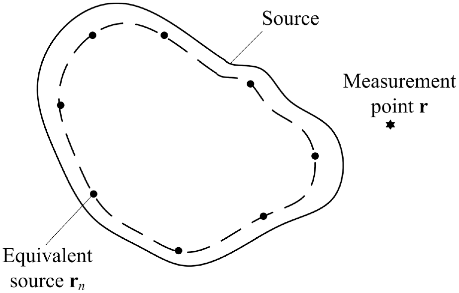
Geometry of the source, the equivalent sources and the measurement point.

where $\rho$ is the density of the medium, c is the sound speed, k is the wave number, N is the total number of the equivalent sources, n is the nth equivalent source, $q({\mathbf{r}}_n)$ is the equivalent source strength at point ${\mathbf{r}}_n$ and $g(\mathbf{r},{\mathbf{r}}_n)$ is the free-field Green’s function defined as

$$g(\mathbf{r},{\mathbf{r}}_n)=\frac{e^{\mathrm{j}k|\mathbf{r}-{\mathbf{r}}_n|}}{4\pi |\mathbf{r}-{\mathbf{r}}_n|}$$

(2)

Assuming the number of measurement points on the holographic surface is M, then the measured pressure can be expressed in a matrix form as

$${\mathbf{p}}_h=\mathbf{Gq}.$$

(3)

where ${\mathbf{p}}_h=[p(r_{h1}),p(r_{h2}),...,p(r_{\mathrm{hM}}){]}^T$ is the column vector consists of the measured pressure, $\mathbf{q}=[q({\mathbf{r}}_1),q({\mathbf{r}}_2),...,q({\mathbf{r}}_N){]}^T$ is the column vector that contains the equivalent source strengths, G is the transfer matrix with the element of $\mathbf{G}(m,n)=g({\mathbf{r}}_m,{\mathbf{r}}_n)$ , ${\mathbf{r}}_m$ and ${\mathbf{r}}_n$ is the location vectors of the mth measurements and nth equivalent source, respectively.

In conventional ESM, the equivalent source strengths with minimum ${\ell }_2\mathrm{-}\mathrm{norm}$ is obtained by solving the following minimization problem

$$\underset{\mathbf{q}}{\mathrm{argmin}}\Vert \mathbf{q}{\Vert }_2\mathrm{subject}\mathrm{to}\Vert \mathbf{p}-\mathbf{Gq}{\Vert }_2\le \epsilon ,$$

(4)

where ε is the data fidelity constraint. In practice, the Tikhonov regularization is usually used to seek the solution of the following minimization problem

$$\underset{\mathbf{q}}{\arg min}\Vert {\mathbf{p}}_h-\mathbf{Gq}{\Vert }_2^2+\lambda \Vert \mathbf{q}{\Vert }_2^2$$

(5)

where λ is the regularization parameter. When the sound source is spatially sparse or close to sparse, the corresponding equivalent source strength is also sparse.^21,22 Then the sparse regularization can be applied to ESM and equation (3) can be solved in the following form

$$\underset{\mathbf{q}}{\mathrm{argmin}}\Vert \mathbf{q}{\Vert }_1\mathrm{subjcet}\mathrm{to}\Vert \mathbf{p}-\mathbf{Gq}{\Vert }_2\le \epsilon$$

(6)

where ε is empirically chosen according to the given signal-to-noise ratio (SNR). Equation (6) is the basic formulation of S-ESM. Compared with ESM, the equivalent source strengths obtained by S-ESM is spatial sparse rather than spatial continuous, leading to a relatively high resolution acoustic imaging and a better performance in reconstruction of the sound field radiated by the spatially sparse source.

R-ESM

Although S-ESM can enhance the resolution of acoustic imaging, the performance of S-ESM is not that good at low frequencies or low SNR. To overcome the restriction, reweighted l₁ minimization is introduced to ESM and R-ESM is proposed in this study. Different from S-ESM, R-ESM utilizes reweighted l₁ minimization to deal with the ill-posed inverse problems of equation (3). The steps of R-ESM are as follows:

Initialization: Set the elements of reweighted coefficient vector $w_i^{(0)}=1,i=1,...,n$ . Set J = 1.

Repeat until convergence (stopping rule):

• Step 1: Solving the following ${\ell }_1$ minimization problem

$$\underset{\mathbf{q}}{\mathrm{agr}min}\Vert {\mathbf{w}}^s{\mathbf{q}}^s{\Vert }_1\mathrm{s}.\mathrm{t}.\Vert {\mathbf{p}}_h-{\mathbf{G}}_{\mathrm{hp}}{\mathbf{q}}^s{\Vert }_2^2\le \epsilon$$

(7)

• Step 2: Updating the reweighted coefficient vector

$$w_i^{s+1}=\frac{1}{\left|q_i^s\right|+\delta }$$

(8)

Set J = J + 1

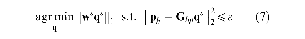
Equation (7) is the basic formulation of R-ESM. Since R-ESM is solved based on a loop iteration of sparse regularization and the update of reweighted coefficient vector. Therefore, compared with R-ESM, S-ESM can be comprehended as the R-ESM with the iteration number of 1 and the equivalent source strength has an effect on the reweighted coefficient in the next iteration. Therefore, the performance of R-ESM is related to that of S-ESM. In the reweighted coefficient vector updating stage, the introduction of parameter $\delta >0$ in equation (8) is to ensure the existence of the reweighted coefficient $w_i^{s+1}$ since the source strengths at some points maybe 0. Since the smaller equivalent source strength will lead to higher reweighted coefficient, the resolution of acoustic imaging can be improved after reweighted iteration.

Simulation

Two-dimensional source localization

In the simulation, two monopoles are selected as the sound sources, and the monopoles S₁ and S₂ are located at (−0.05, 0, 0 m) and (0.05, 0, 0 m) respectively. The diagram of the simulation is shown in Figure 2. The reconstruction and holographic planes are located 0.03 and 0.09 m away from the source, respectively. The pressures on the two planes are measured with the same dimension of 0.05 × 0.05 m² and the interspacing of 0.05 m, ranging from −0.25 to 0.25 m. The equivalent sources are distributed on the source plane. Gaussian white noise with SNR of 20 dB is added to the pressures on the holographic plane by using the Matlab function awgn.

Figure 2.

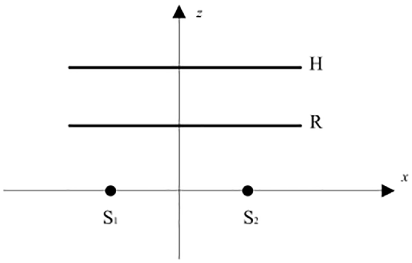
The diagram of the simulation.

To quantitatively evaluate the performance of the methods, the reconstruction error is defined as

$$\mathrm{Error}=\frac{{\Vert {\mathbf{s}}_{\mathrm{cal}}-{\mathbf{s}}_{\mathrm{th}}\Vert }_2}{{\Vert {\mathbf{s}}_{\mathrm{th}}\Vert }_2}\times 100\%,$$

(9)

where ${\mathbf{s}}_{\mathrm{cal}}$ is the reconstructed pressure or source strength, and ${\mathbf{s}}_{\mathrm{th}}$ is the theoretical pressure or source strength.

The comparison between the reconstructed pressure and theoretical one at 200 Hz are illustrated in Figure 3. The pressures reconstructed by S-ESM and R-RESM both match the theoretical one well, with the corresponding reconstruction errors of 8.73% and 1.27%, respectively. This indicates that both the two methods can provide a high reconstruction accuracy. The reconstruction errors of pressure versus frequency are shown in Figure 4. On the whole frequency range, both the two methods can reconstruct the sound field with a high accuracy. Meanwhile, the effect of position of measurement plane on the performance of the two methods is also analyzed and the result is shown in Figure 5. Although the two methods can provide an accurate reconstruction of pressure, the error of R-ESM is always lower than that of S-ESM, indicating better performance of R-ESM for spatially sparse sources. Since both S-ESM and R-ESM can provide an accurate reconstruction of the sound field radiated by the spatially sparse sources, in what follows, the performance of S-ESM and R-ESM in sound field reconstruction is not analyzed.

Figure 3.

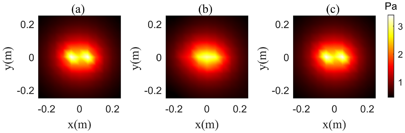
The pressures on the reconstruction plane at 200 Hz. (a) the theoretical values, the pressures reconstructed by (b) S-ESM and (c) R-ESM.

Figure 4.

Reconstruction errors of S-ESM and R-ESM versus frequency.

Figure 5.

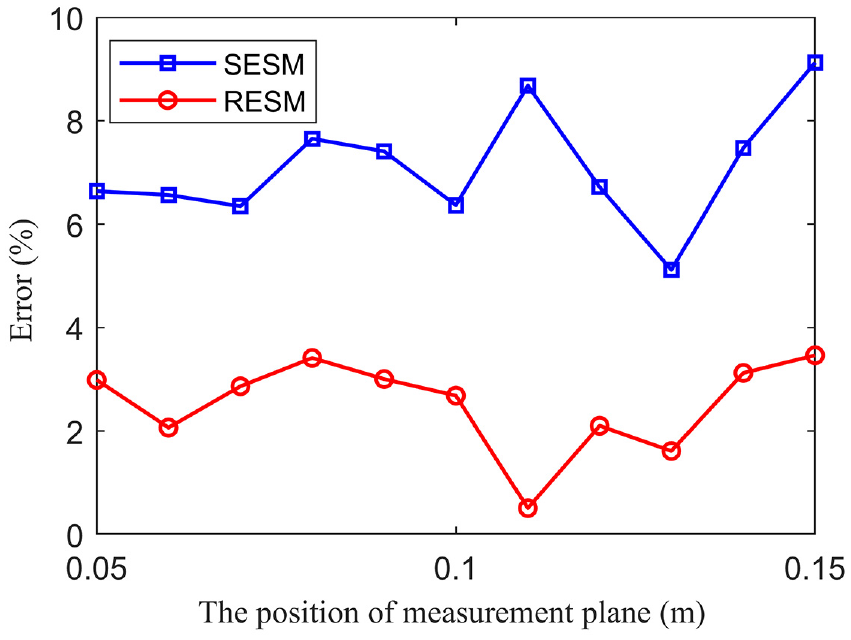
Reconstruction errors of S-ESM and R-ESM versus the position of measurement plane.z

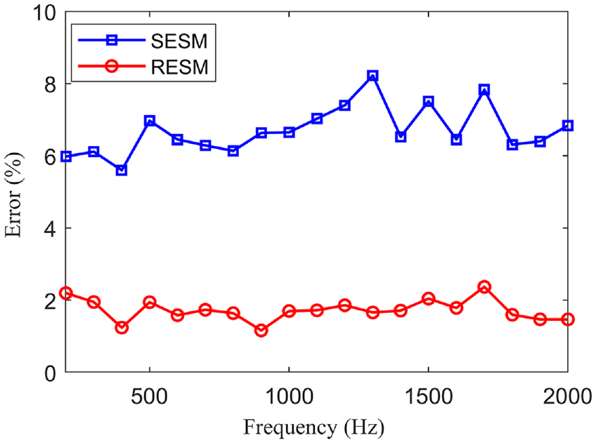
In order to realize a higher resolution of acoustic imaging, the obtained equivalent source strengths are used to locate the sound sources. The equivalent source strengths obtained by the two methods at 200 and 1000 Hz are shown in Figures 6 and 7, respectively. The amplitudes of the equivalent source strengths given in the simulation are normalized to 1. It can be seen that S-ESM can distinguish the two sources at 1000 Hz. However, when the frequency decreases down to 200 Hz, the method fails to separate the two sources. By contrast, R-ESM can provide a lower side lobe and locate the two sources with higher spatial resolution after reweighted iteration at the two frequencies. The reconstruction errors of the equivalent source strengths of S-ESM and R-ESM versus frequency are illustrated in Figure 8. It can be concluded that the error of S-ESM decreases with the increase of frequency, which is probably due to the low spatial resolution of S-ESM for low-frequency sound sources. By comparison, the error of R-ESM is lower and more stable than that of S-ESM in the whole frequency range.

Figure 6.

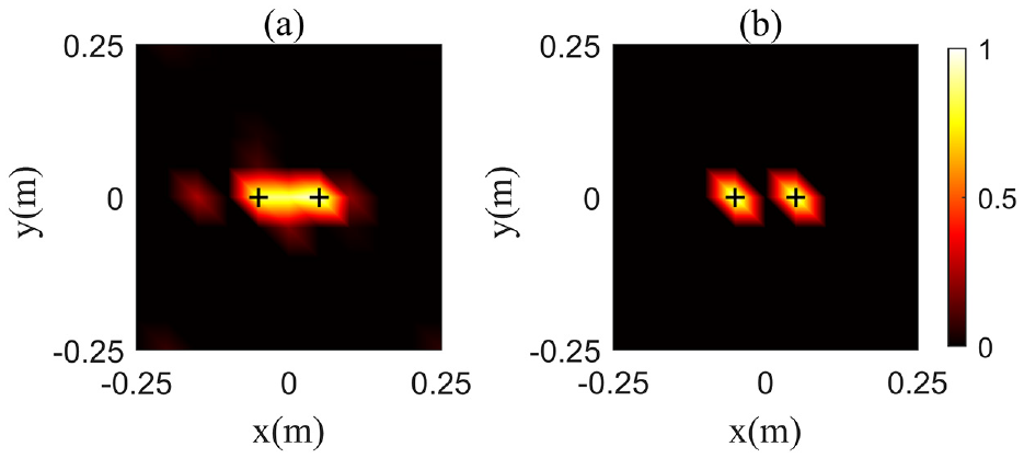
The distribution of the equivalent source strengths obtained by (a) S-ESM, (b) R-ESM at 200 Hz. The two “+” denotes the locations of the two sources.

Figure 7.

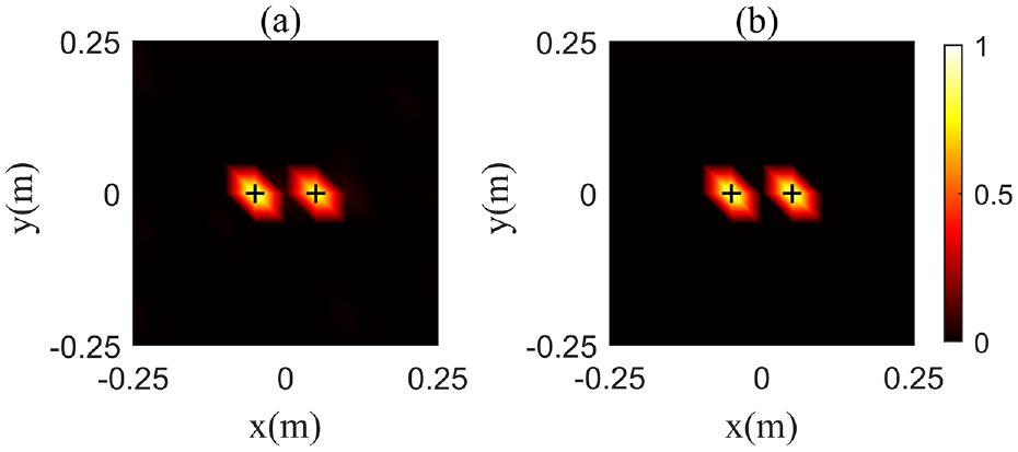
The distribution of the equivalent source strengths obtained by (a) S-ESM, (b) R-ESM at 1000 Hz. The two “+” denotes the locations of the two sources.

Figure 8.

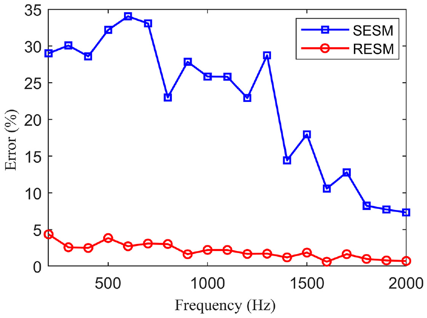
Reconstruction errors of S-ESM and R-ESM versus frequency.

Three-dimensional source localization

The second simulation is conducted to analyze the localization performance of the equivalent source strengths in three dimensions, that is, the sound sources are not distributed on the same plane. The diagram of the simulation is shown in Figure 9. The three monopoles S₁, S₂, and S₃ are located at (0.05, 0, −0.1 m), (0.05, 0, 0 m), and (0.15, 0, 0 m) respectively. Holographic plane H₁ is perpendicular to the z-axis, located at the plane with the coordinate in z direction of zh₁ = 0.1 m. The coordinate ranges of H₁ in x and y directions are both −0.25∼0.25 m. Holographic plane H₂ is perpendicular to the x-axis, located at the plane with the coordinate in x direction of xh₂ = −0.1 m. The coordinate range of H₂ in the y direction is −0.25∼0.25 m and that in z direction is −0.25∼0 m. The measurement intervals on the two holographic planes are both 0.05 m. A total of 187 points of sound pressure data were measured. To identify the source location in three dimensions, the equivalent source plane is arranged on five planes with the coordinates in z direction of −0.2 m (E₁), −0.15 m (E₂), −0.1 m (E₃), −0.05 m (E₄), and 0 m (E₅), with the coordinate range of 0∼0.25 m in x direction and −0.25∼0.25 m in y direction. A total of 330 equivalent sources are arranged on the five equivalent source planes, and the holographic pressure is added with random noise with a SNR of 30 dB.

Figure 9.

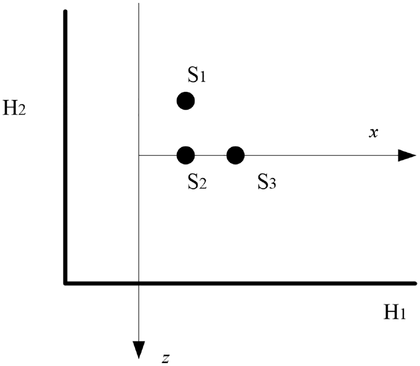
The diagram of the simulation.

The distributions of the equivalent sources on each plane obtained by S-ESM and R-ESM at 500 and 1500 Hz are shown in Figures 10 and 11, respectively. At 500 Hz, the equivalent source strengths obtained by S-ESM on plane E₁ and E₂ are all closed to 0. Meanwhile, it achieves peaks at the points (0.05 m, 0 m) on plane E₃ and (0.05 m, 0 m) and (0.15 m, 0 m) on plane E₅, corresponding to the coordinates of sources S₁, S₂, and S₃, indicating that S-ESM can locate the source S₁ on the plane E₃ and can separate the sources S₂ and S₃ on plane E₅. However, it should be noted that there also exists a virtual source on plane E₄ according to the distribution of equivalent source strengths obtained by S-ESM, indicating that S-ESM cannot distinguish the sources S₁ and S₂ in z direction. By comparison, after reweighted iteration, R-ESM can completely separate the three sources, which improves the spatial resolution of S-ESM in three-dimensional localization of sound sources. When the frequency increases up to 1500 Hz, both the two methods can separate the three sources. The reconstruction errors of the equivalent source strengths of S-ESM and R-ESM versus frequency are illustrated in Figure 12. With the increasement of frequency, the error of S-ESM decreases accordingly and trends to be stable when the frequency is above 1000 Hz. By comparison, the error of R-ESM is lower and more stable than that of S-ESM on the whole frequency range.

Figure 10.

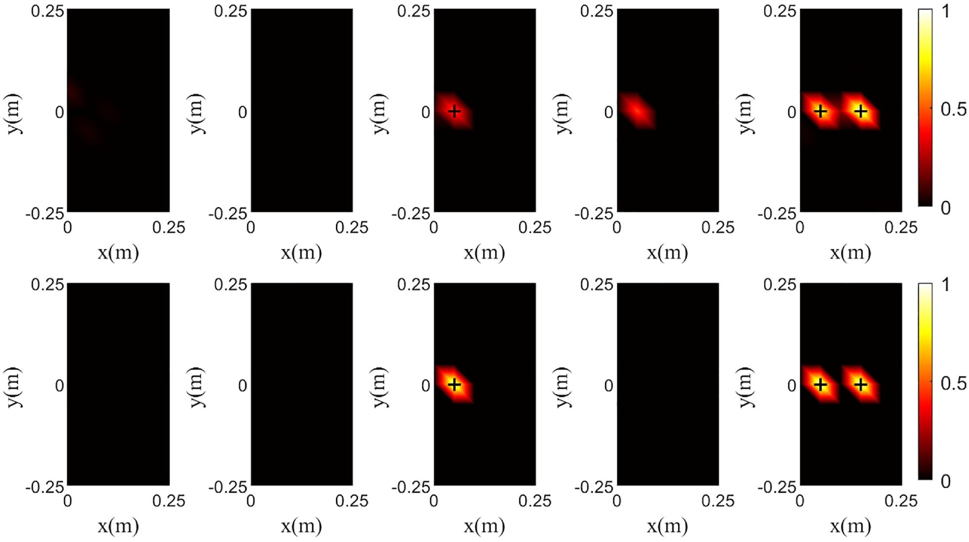
Comparison of the equivalent source strengths at 500 Hz. Top row: S-ESM, bottom row: R-ESM. Column from left to right: E₁, E₂, E₃, E₄, E₅. The three “+” denotes the locations of the three sources.

Figure 11.

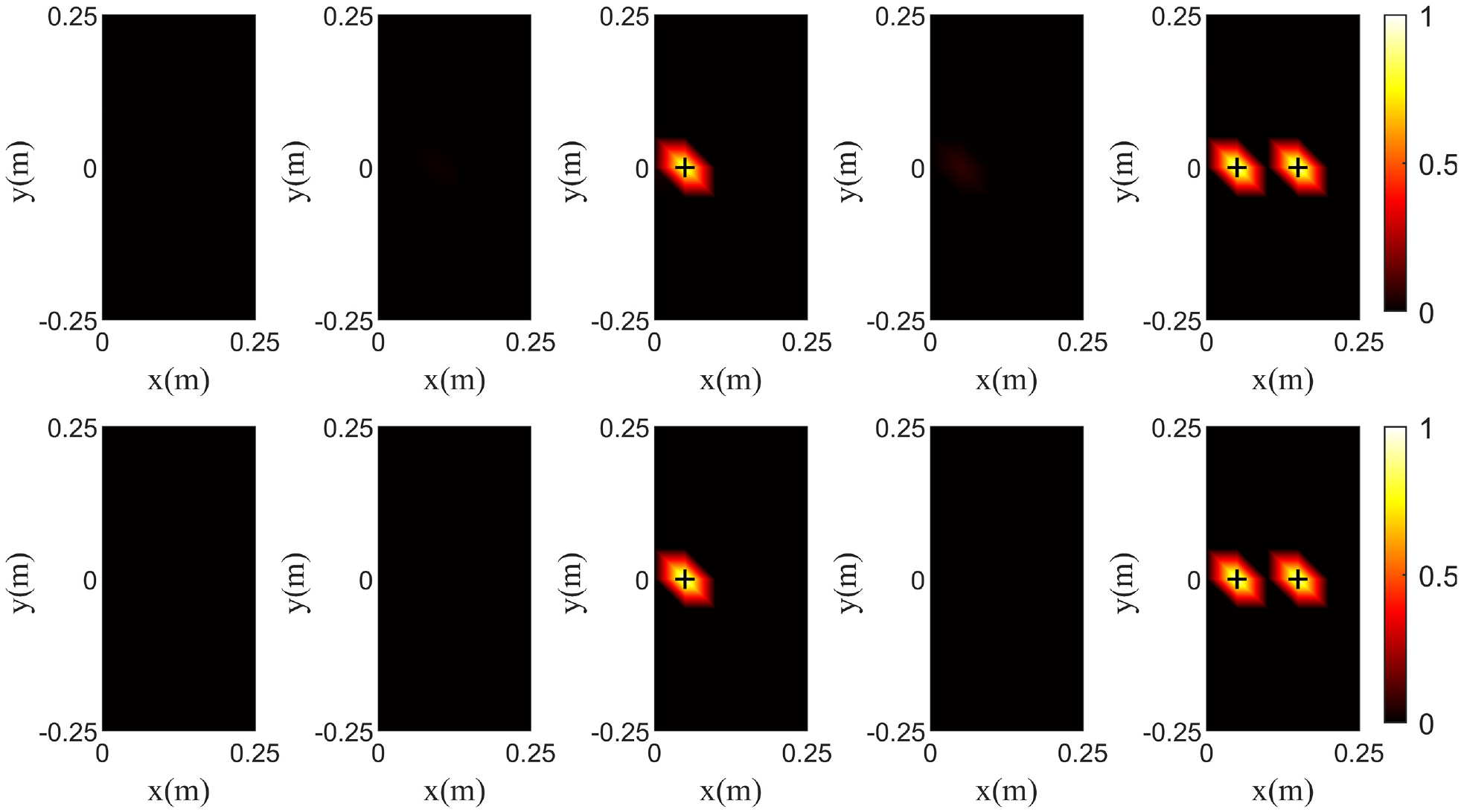
Comparison of the equivalent source strengths at 1500 Hz. Top row: S-ESM, bottom row: R-ESM. Column from left to right: E₁, E₂, E₃, E₄, E₅. The three “+” denotes the locations of the three sources.

Figure 12.

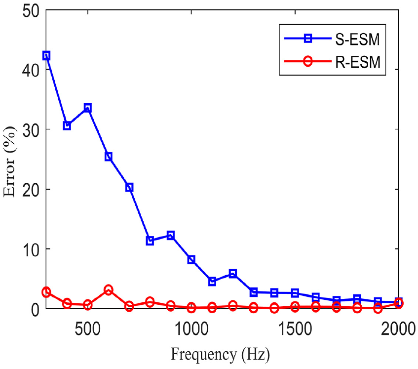
Reconstruction errors of S-ESM and R-ESM versus frequency.

Experiment

Two experiments were conducted in a semi-anechoic chamber. The first experimental setup is shown in Figure 13(a). Two loudspeakers are selected as the sound sources, which located at (0, 0, 0 m) and (0.1, 0, 0 m) respectively. The loudspeakers are driven by the signal generated by the computer with the frequency of 200 Hz. The holographic pressure is measured through scanning on the holographic plane by a linear array composed of 11 microphones. The holographic plane is 0.05 m away from the loudspeakers. The dimension of the holographic plane is 0.5 × 0.5 m², with the measurement interval of 0.05 m. The equivalent source plane is arranged on the same plane as the speaker. Same with that in the simulations, the amplitudes of the equivalent source strengths given in the experiments are normalized to 1.

Figure 13.

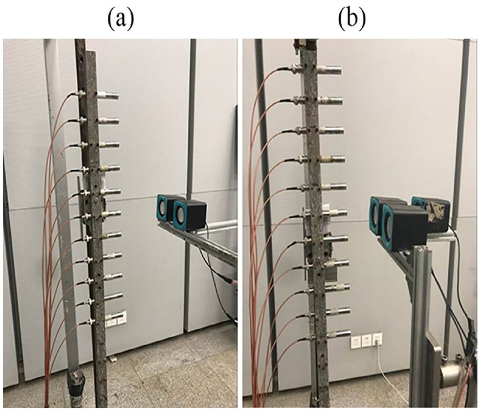
Photograph of the experimental setups: (a) The first experiment; (b) The second experiment.

Figure 14 shows the spatial distribution of equivalent source strengths obtained by S-ESM and R-ESM at 200 Hz. It can be seen that although the peaks of the equivalent source strengths obtained by S-ESM correspond to the positions of the loudspeakers, the side lobe of S-ESM is wider than that of R-ESM. By contrast, R-ESM can separate the two sources completely, and the spatial resolution is significantly improved.

Figure 14.

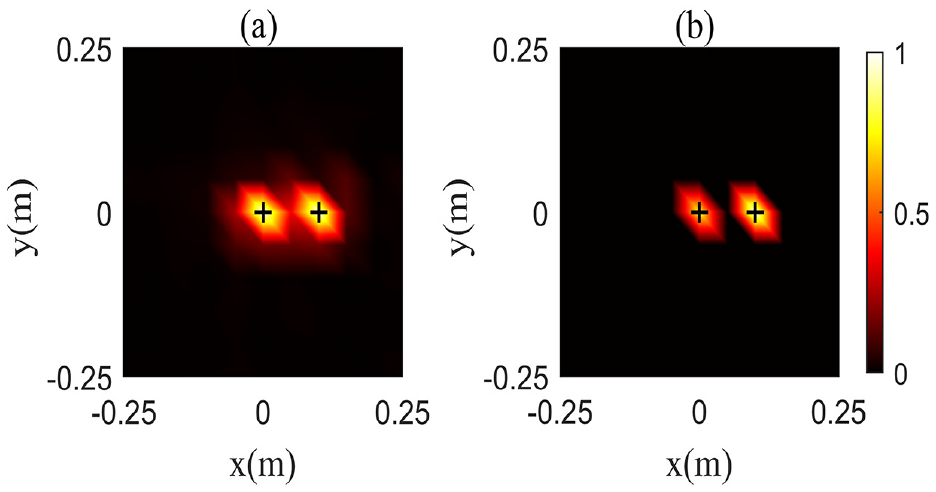
The distribution of the equivalent source strengths obtained by (a) S-ESM, (b) R-ESM at 200 Hz. The two “+” denotes the locations of the two sources.

The second experimental setup is shown in Figure 13(b). The three loudspeakers S₁, S₂, and S₃ are selected as the sound sources, located at (0, 0, −0.1 m), (0, 0, 0 m), and (0.1, 0, 0 m) respectively. The loudspeakers are driven by the signal generated by the computer with the frequency of 500 Hz. The holographic pressure is measured through scanning on the holographic plane by a linear array composed of 11 microphones. Holographic plane H₁ is perpendicular to the z-axis, located at the plane with the coordinate in z direction of zh₁ = 0.05 m. The coordinate ranges in x and y directions are both −0.25∼0.25 m. Holographic plane H₂ is perpendicular to the x-axis, located at the plane with the coordinate in x direction of xh₂ = −0.05m. The coordinate range in y direction is −0.25∼0.25 m and that in z direction is −0.25∼0 m. The measurement intervals on the two holographic planes are both 0.05 m. A total of 187 points of sound pressure data on two holographic planes were measured. The equivalent source planes are arranged on five planes with the coordinate in z direction of −0.2 m (E₁), −0.15 m (E₂), −0.1 m (E₃), −0.05 m (E₄), and 0 m (E₅), with the coordinate range of 0∼0.25 m in x direction and −0.25∼0.25 m in y direction. A total of 330 equivalent sources are distributed on the five equivalent source planes.

The distribution of the equivalent sources on each plane obtained by S-ESM and R-ESM at 500 Hz is shown in Figure 15. The result is similar to that in the simulations, the amplitude of the equivalent source strengths obtained by S-ESM are close to 0 on planes E₁, E₂, and E₄. The peak of the equivalent source strengths on plane E₃ is consistent to the position of source S₁. However, the resolution of equivalent source strengths on plane E₁ is not high enough to separate sources S₂ and S₃. By comparison, R-ESM can promote the resolution of the result by means of reweighted iteration and the three sources can be identified from the equivalent source strengths.

Figure 15.

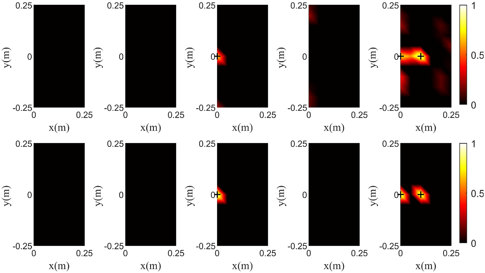
Comparison of the equivalent source strengths at 500 Hz. Top row: S-ESM, bottom row: R-ESM. Column from left to right: E₁, E₂, E₃, E₄, E₅. The three “+” denotes the locations of the three sources.

Conclusion

Sparse regularization has been applied to ESM in order to improve the acoustic imaging resolution. However, the application is not valid at low frequencies. To deal with the issue, reweighted l₁ minimization is introduced to ESM. Different from S-ESM, R-ESM takes advantage of reweighted l₁ minimization to deal with the ill-posed inverse problems rather than sparse regularization. In R-ESM, the equivalent source strength has an effect on the reweighted coefficient in the next iteration. Since the smaller equivalent source strength will lead to higher reweighted coefficient, the resolution of acoustic imaging can be improved after reweighted iteration. The numerical results demonstrate that compared with S-ESM, R-ESM can provide a low side lobe and higher spatial resolution imaging of sound source distribution. Meanwhile, to realize the acoustic imaging in three-dimensional sound field, the equivalent sources are arranged in three-dimensional space and R-ESM can be utilized to promote the resolution. The results of two experiments further validate these findings.