
Abstract
In order to solve the problems of spatial resolution limit and reduce the measurement cost, the compressive sensing theory and the sparse regularization are applied to the near-field acoustic holography (NAH) technology. In the previous works, the Equivalent Source Method (ESM)-based NAH has been extended in the sparsity framework by sampling the sound pressure signals sparsely. However, this Compressive ESM (CESM) mode would suffer from the low precision problem in the particle velocity reconstruction. To improve the reconstruction accuracy of the particle velocity, this paper is going to take the sparse particle velocity as the input of NAH to establish a new CESM mode based on the particle velocity measurement. In the meantime, the number of sampling points will be reduced greatly without losing the reconstruction accuracy when compared to the conventional ESM with the Tikhonov regularization based on the particle velocity measurement. Several numerical simulation experiments have been carried out to examine the performance of the proposed model. The results show that the proposed model delivers a satisfactory performance in the reconstruction of both the pressure and particle velocity on the condition that the number of sampling points is much smaller than that of the conventional ESM, and the proposed model performs much better than the existing CESM mode based on the sound pressure measurement especially when reconstructing the particle velocity.
Keywords
Introduction
Near-field acoustic holography (NAH) can provide high spatial resolution in sound field reconstruction,1–3 but it is limited by Nyquist sampling theorem, resulting that the total number of sampling points may be excessive. As a result, either a large measurement array with corresponded acquisition equipment or a lot of time for the measuring process is required, that is, the conventional NAH requires high measurement cost, which is especially true in the middle and high frequency range.
In 2012, Chardon et al. applied the compressive sensing (CS) theory to NAH technology and obtained satisfactory reconstructed results with a small number of sampling points. 4 They succeeded in reducing the number of measurement points without losing the reconstruction accuracy because of the CS theory, in which the signal can be reconstructed accurately from a limited number of measurement points by using the sparse regularization. Since then, more and more researches begin to pay attention to the application of the CS theory and the sparse regularization in the NAH technology.
Hald and Fernandez-Grande et al. successively introduced the application of CS theory in the Equivalent Source Method (ESM)-based NAH technology in the Conference of Inter-Noise.5,6 They used sparse regularization to replace conventional Tikhonov regularization and establish Compressive ESM (CESM), providing higher reconstruction accuracy than conventional ESM. Then Fernandez-Grande et al. analyzed the influence of the correlation of the column vectors of the transfer matrix in CESM on the reconstruction results and obtained stable and high-precision reconstruction results. 7 And Hald studied the sparse regularization algorithm through comparing the computational efficiency of five sparse regularization iterative methods, and gave the application conditions of different sparse regularization algorithms to further ensure the robustness of CESM and higher reconstruction accuracy. 8 However, CESM is applied on the premise that the signal to be reconstructed is spatial sparse, that is, the sound source is required to be spatial compact. If the sound source is spatially distributed and continuous, the CESM model may not reconstruct the sound field accurately, or even fail in reconstructing the field.
In order to solve the problem that the sparse basis is not applicable to CESM when facing the spatially distributed sound sources, Bi and Liu derived the sound radiation modes of equivalent source strength through ESM and regarded the modes as the sparse basis to propose a Compressive Modal ESM (CMESM). 9 Furthermore, Liu et al. constructs a redundant dictionary for the equivalent source strength by using both CESM and CMESM orthogonal basis functions, and used the dictionary as the sparse basis. 10 They found that this model based on the redundant dictionary performed well for both the compact and distributed sources, enhancing the applicability of the technology for different types of the source with more stable and accurate reconstruction results. Then, Liu et al. and Bi et al. used the Boundary Element Method (BEM) to deduce the acoustic radiation modes as a sparse basis to reconstruct the particle velocity on the surface of the vibrating body, and found that a relatively high vibration velocity reconstruction accuracy could still be obtained with a small number of sampling points.11,12 In addition, Hu et al. performed singular value decomposition on the transfer matrix, and then used the input mode representing the source or the output mode representing the velocity as the orthogonal basis function to construct a sparse basis for the spatially distributed sources. 13 Combining with the sparse basis functions of CESM, He et al. constructs an equivalent redundant dictionary, which can be applied to both spatially sparse and spatially distributed sources. 14 For spatially distributed sources, Hald compared the CESM and its various modified algorithms, and gave the applicability of various algorithms for different types of sound sources. 15
On the other hand, Fernandez-Grande and Daudet proposed a block sparse regularization to solve the adaptive problem of spatially distributed continuous sound sources 16 ; and Bai et al. proposed an iterative algorithm to solve the block sparse constraint problem. 17 In 2022, Bi et al. combined the block sparse with the sparse Bayesian learning (SBL) algorithm, which is easier to obtain the sparsest solution than the l1–norm minimization algorithms embedded in the sparse regularization above and has been widely used in the fields of acoustic localization,18–23 to accurately reconstruct the sound field radiated from different types of sound sources by adjusting the size of the sound source block. 24
To expand the application of CS theory in NAH technology, some scholars have begun to study the application of CS theory in NAH technology of non-free sound field. In 2016, Fernandez-Grande and Xenaki applied sparse regularization to sound field reconstruction based on the sparsity hypothesis of sound field signal decomposition under plane wave basis function, and the results showed that sparse regularization had better reconstruction accuracy and spatial resolution than Tikhonov regularization. 25 Verburg et al. and Fernandez-Grande et al. applied the CS theory to indoor sound field reconstruction, and obtained good reconstruction results.26,27 For the complex closed sound field with high frequency, Hahmann et al. used the local representations and explored data-driven approaches to obtain suitable models and found that the local partitioning models conform to fields of high spatial complexity. 28 In 2017, Wang and Chen reconstruct the sound field in cylindrical cavity at low frequency by combining sparse regularization with the least square solution of the Helmholtz equation. 29 However, this method is only suitable for the sound field in cylindrical cavity, and the resolution is relatively low. Subsequently, Hu et al. applied the sparse equivalent source algorithm based on transfer matrix mode to the inner space sound field, which can be applied to any shape of sound source with relatively high computational efficiency. 13 In addition, Bi et al. applied sparse regularization to sound field separation technology, constructing sparse bases with equivalent source strength for target sound source and interference sound source respectively. 30 And they studied the dependence of this technology on SNR and sampling points, finding that the sound field separation technology based on redundant dictionary can guarantee high separation accuracy and has the best anti-noise performance when facing different types of sound sources.
However, the techniques above mainly focus on the measurement and reconstruction of sound pressure, named as CESM-p, which cannot provide reasonable results when the particle velocity is desired to be reconstructed because the transfer function in the process of solving the sound source is concerned with the pressure but the transfer function in the sound field reconstruction is concerned with the particle velocity, as shown in Figure 1. A number of literatures have shown that the NAH based on the particle velocity measurement is superior to that based on the sound pressure measurement when reconstructing the particle velocity.31–33
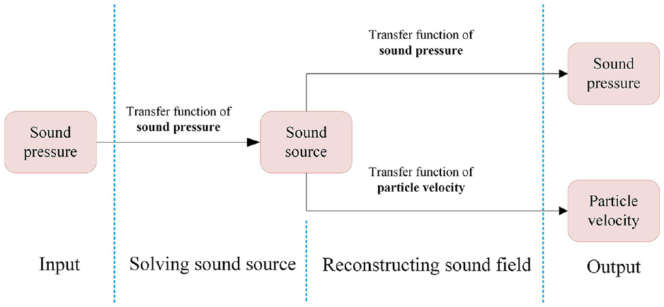
The block diagram representation of the CESM/ESM based on the sound pressure measurement.
In order to solve the low precision problem of particle velocity reconstruction when using the CESM-p, this paper is going to combine the CS theory with the particle velocity measurement instead of the sound pressure measurement and use the particle velocity as the input to establish a new CESM model, named as CESM-v, as shown in Figure 2. According to Jacobsen and Jaud 31 , Pezerat et al. 32 and Zhang et al., 33 it can be expected that the proposed CESM-v model would improve the particle velocity reconstruction accuracy to a great extent when compared to the CESM-p, and the number of sampling points could be much smaller than that of the conventional ESM on the premise of guaranteeing reconstruction accuracy.
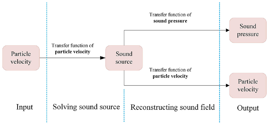
The block diagram representation of the CESM/ESM based on the particle velocity measurement.
The rest of the paper is organized as follows. Section II reviews the theory of CESM-p and follows the introduction of the theory of proposed CESM-v. Section III examines the performance of the proposed CESM-v through the particle velocity and sound pressure reconstruction on the basis of the numerical simulation results. Finally, Section IV presents the conclusions of the study.
Theoretical background
CESM based on the pressure measurement (CESM-p)
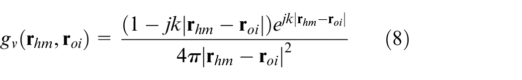
Considering the near-field of an acoustic source, the sound pressure at an arbitrary point
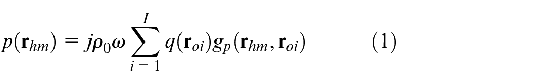
where
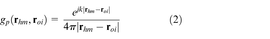
where
Given that there are measurement points forming the hologram surface, the equation (1) can be written in a matrix form as

where
According to the measured holographic pressure
where
where
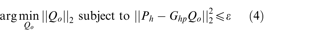
When the underlying problem is sparse, the CS theory can be utilized and the solution of equation (3) can be solved through
Equation (6) is the CESM model based on the pressure measurement (CESM-p).
CESM based on the particle velocity measurement (CESM-v)
According to Jacobsen and Jaud 31 , Pezerat et al. 32 and Zhang et al., 33 the performance of NAH is generally not that good when the sound pressure is used as the holographic input to reconstruct the particle velocity, especially when the ESM is used as the holographic algorithm. 33 In this paper, the particle velocity will be measured as the holographic data to establish a new CESM model, that is, CESM-v.
Similar to CESM-p model, if a particle velocity sensor is placed at any point
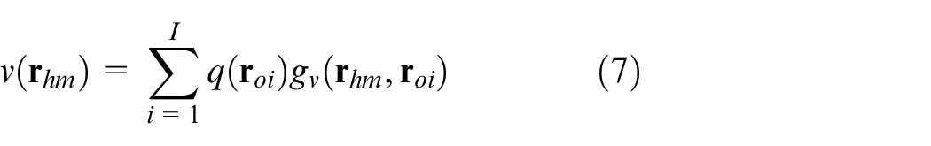
where
Considering there are M sampling points on the measurement surface, the particle velocities in equation (7) would be a vector and can be formulated as

where
where
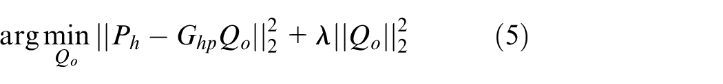
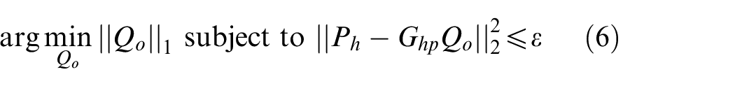
With the measured normal particle velocity
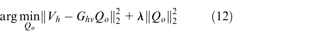
Also, the Tikhonov regularization is used to solve the ill-posed inverse problem to reduce the influence of the measurement error
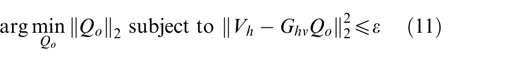
Inspired by the idea of CESM-p, the normal particle velocity on the measurement surface could also be sparsely sampled, and the sparse regularization could be adopted to obtain the sparse source strength vector by solving the
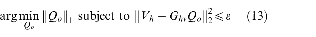
Equation (13) is the CESM model based on the particle velocity measurement (CESM-v). Substituting the obtained sparse equivalent source strength
Numerical simulation experiments
Reconstruction of the particle velocity
To examine the effectiveness of the proposed CESM-v model in reconstructing the sound field, a pulsing sphere with a radius of 0.05 m was used to carry out several numerical simulation experiments. Taking the center of the sphere source as the origin, a Cartesian coordinate system was established. The hologram surface was parallel to the xOy plane with 0.07 m away from the sphere source, and the hologram grid points distributed from −0.25 to 0.25 m in both x and y directions with the interval of 0.05 m, that is, there are 121 gird points on the hologram surface. The normal particle velocity at each measured point on the hologram surface was given as
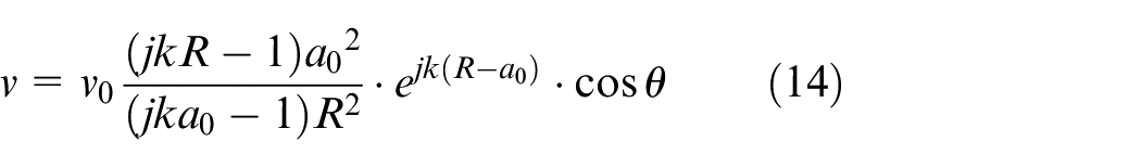
where
The reconstruction surface as well as the equivalent source surface was conformal with the hologram surface with the same aperture and interval. They were located at
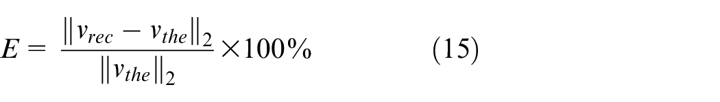
where
Since the CESM-v model is based on the sparse sampling of the particle velocity, we need to select some sampling points randomly from the 121 grid points presenting a regular array on the hologram surface. Here the number of the sampling points used is 60. Figure 3 gives one of the random sampling arrays. With the normal particle velocity sampled sparsely, the normal particle velocity at 1000 Hz on the reconstruction surface is reconstructed by using the proposed CESM-v model, and the result is shown in Figure 4, where the theoretical normal particle velocity computed with equation (14) is also given, acting as the reference. For comparison, the CESM-p model is also used to reconstruct the normal particle velocity and the reconstructed result is given in Figure 4. The sparse sampled sound pressure used in the CESM-p model was given as
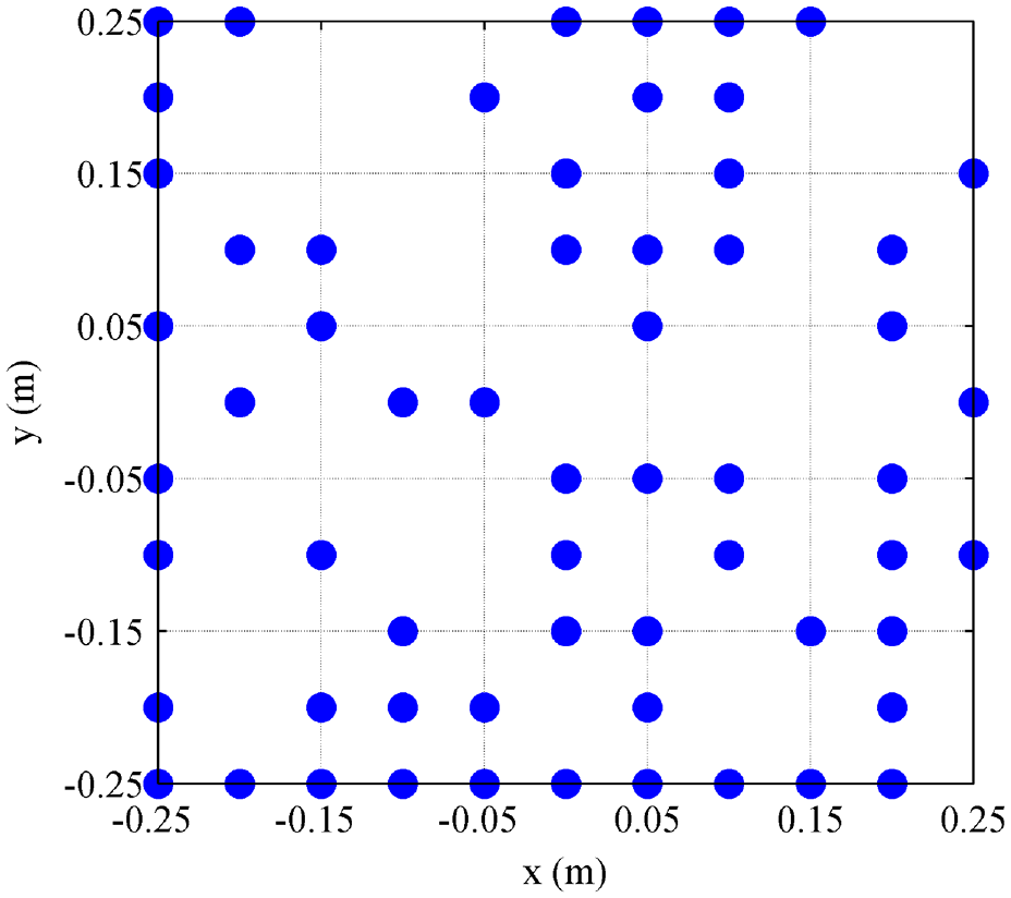
The 60 random sampling points in the traditional regular array.
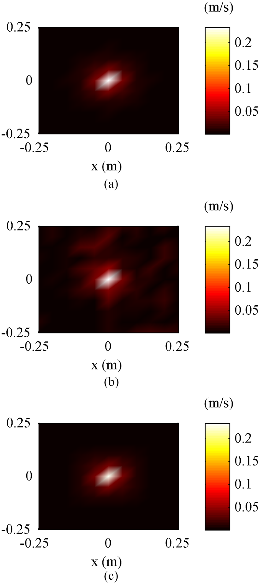
The reconstructed and theoretical normal particle velocities at 1000 Hz: (a) theoretical value, (b) obtained by using CESM-p-60, and (c) obtained by using CESM-v-60. (60 means the number of sampling points).
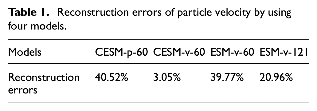
From Figure 4, it can be seen that the reconstructed normal particle velocity obtained by using the CESM-v model distributes smoothly and agrees well with the theoretical value, while the reconstructed result obtained by using the CESM-p model shows some pseudo peaks around the real peak, thus performing some deviation from the theoretical value. To compare the performance of the CESM-v and CESM-p model more intuitively, the normal particle velocity reconstruction errors are given in Table 1. It can be easily found that the reconstruction error of CESM-v is only 3.05%, while error of CESM-p is up to 40.52%. As expected, the proposed CESM-v model does reconstruct the particle velocity better than the CESM-p model.
Reconstruction errors of particle velocity by using four models.
To better demonstrate the superiority of the CESM-v over the CESM-p, Figure 5 gives the equivalent source strengths obtained by using the two models. It can be found that the equivalent source strength obtained by using the CESM-p shows one steep peak as well as some small peaks, but the equivalent source strength obtained by using the CESM-v shows only one steep peak without any other small peak. This illustrates that the source strength obtained by using the CESM-p distributes continuously in space and behaves large sidelobes, resulting in low spatial resolution, although the source can be identified from the peak. However, the spatial distribution of the source strength obtained by using the CESM-v is relatively concentrated, identifying the source more accurately, and thus the CESM-v can provide higher spatial resolution. The results verify that the CESM-v model has advantage over the CESM-p model when the particle velocity is to be reconstructed to identify the sound source.
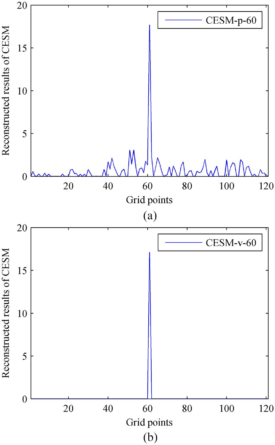
The reconstructed equivalent source strengths at 1000 Hz: (a) obtained by using CESM-p-60 and (b) obtained by using CESM-v-60. (60 means the number of sampling points).
As known, the conventional ESM with the Tikhonov regularization based on the particle velocity measurement, that is, ESM-v, can provide reasonable accuracy in the reconstruction of particle velocity. To verify the effectiveness and superiority of the CESM-v more comprehensively, the ESM-v is also used to calculate the normal particle velocity at 1000 Hz and two cases, 60 and 121sampling points, are considered. The reconstructed results are given in Figure 6. Comparing the amplitude of the reconstructed normal particle velocity, it can be seen that both of the reconstructed results (Figure 6(b) and (c)) are significantly smaller than the theoretical value (Figure 6(a)), but the reconstructed result (Figure 6(c)) obtained when using 121 sampling points is slightly better. Also, the corresponding reconstruction errors are shown in Table 1. It can be seen that the errors of ESM-v are 39.77% when using 60 sampling points and 20.96% when using 121 sampling points, both of which are much larger than 3.05%, the error of CESM-v. It is predictable that the ESM-v when using 60 sampling points performs poorly because there are too few sampling points to acquire sufficient holographic data. However, the ESM-v even if a traditional regular array with 121 sampling points is used cannot reach the same level of accuracy of the CESM-v. This is an exciting and meaningful finding.

The reconstructed and theoretical normal particle velocities at 1000 Hz: (a) theoretical value, (b) obtained by using ESM-v-60, and (c) obtained by using ESM-v-121. (60 and121 mean the number of sampling points).
Meantime, the equivalent source strengths at 1000 Hz are reconstructed by using the ESM-v with 60 and 121 sampling points, and the results are given in Figure 7. It can be found that the source strength obtained when using 60 sampling points shows three or four significant peaks (Figure 7(a)), which would be likely to identify some pseudo sources, thus resulting in failed reconstruction. On the other hand, the source strength obtained when using 121 sampling points is much better, presenting one significant peak with several small peaks (Figure 7(b)), but is still not as smooth as the source strength obtained by using the CESM-v (Figure 5(b)). As a result, ESM-v cannot guarantee the same spatial resolution as the CESM-v. This illustrates once again that CESM-v can provide better results than ESM-v even if sufficient sampling points is used.
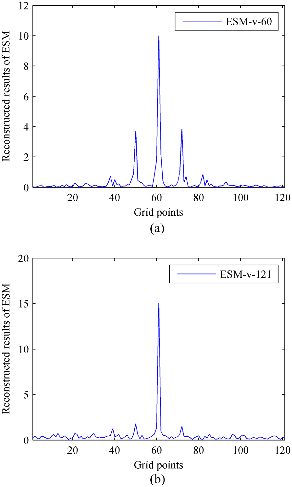
The reconstructed equivalent source strengths at 1000 Hz: (a) obtained by using ESM-v-60 and (b) obtained by using ESM-v-121. (60 and121 mean the number of sampling points).
Furthermore, the reconstruction errors of the normal particle velocity versus the frequency by using the four models above, ESM-v-60, ESM-v-121, CESM-p-60, CESM-v-60, are computed and given in Figure 8. It can be found that ESM-v-60 presents large reconstruction errors, which is predictable because of insufficient holographic data. The ESM-v-121 provides reasonable and stable reconstruction errors, around 18% on the whole frequency band, but it is not as good as CESM-v-60, which gives much smaller reconstruction errors, less than 3% except the largest error 10.61% at 400 Hz.
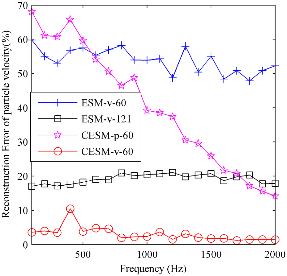
The reconstruction errors of normal particle velocity versus frequency by using four models, ESM-v-60, ESM-v-121, CESM-p-60, and CESM-v-60.
An interesting observation is that the reconstruction errors of CESM-p-60 decrease with the frequency. The reason for this phenomenon may be found from the difference between the sound pressure transfer matrix
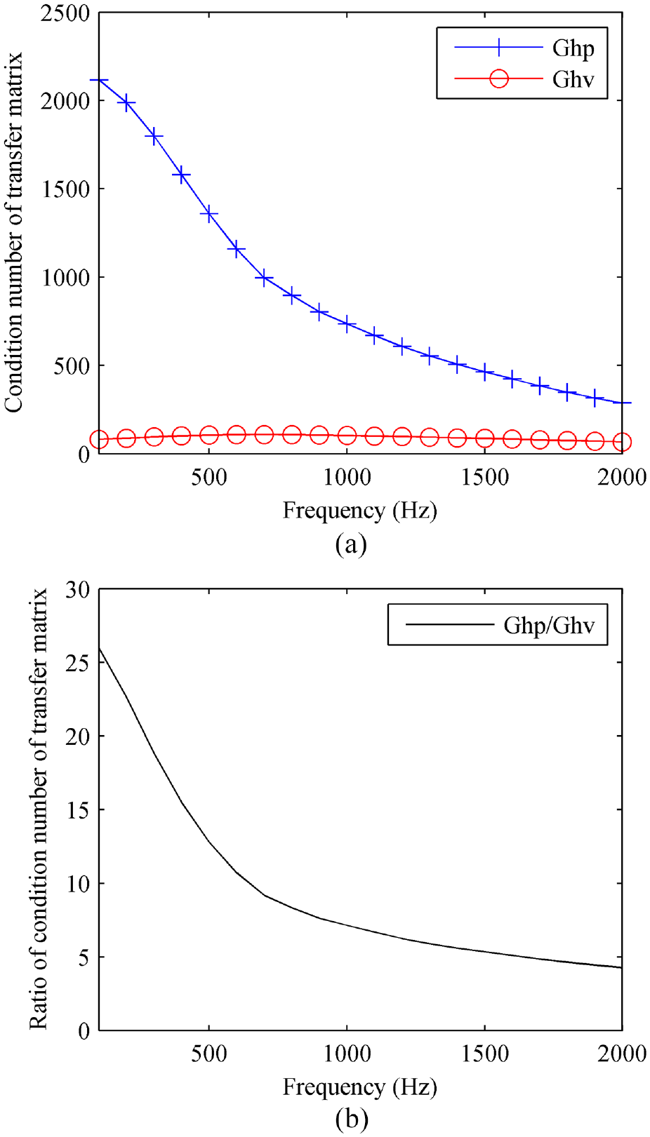
The condition numbers of transfer matrices: (a) the condition numbers of the pressure transfer matrix G_hp and the particle velocity transfer matrix G_hv and (b) the ratio of G_hp to G_hv.
To sum up, the proposed CESM-v model is a good method with high accuracy in reconstructing the particle velocity to identify the sound source. If the sound pressure is reconstructed, what about the reconstruction results? Does the CESM-v model still perform better than CESM-p model? The next subsection presents the analysis of pressure reconstruction.
Reconstruction of the sound pressure
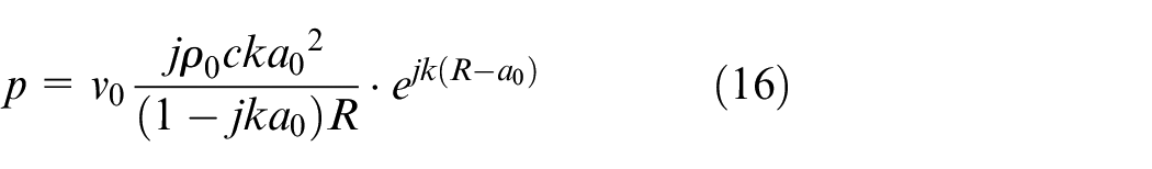
In this subsection, the reconstruction of the sound pressure is analyzed to examine the wide applicability of the proposed CESM-v model. By using the CESM-v as well as the CESM-p, in both of which 60 sampling points are used, the sound pressure at 1000 Hz on the reconstruction surface is calculated and the results are shown in Figure 10. From the figure, it can be seen that the reconstructed values are in good agreement with the theoretical value in both amplitude range and spatial distribution, and the errors of CESM-p and CESM-v are only 2.45% and 1.22%, respectively. At the same time, the conventional ESM with the Tikhonov regularization including ESM-p and ESM-v with 121 sampling points, were also used to reconstruct the sound pressure with the reconstruction errors of 12.73% for the ESM-p and 5.58% for the ESM-v. Since the reconstructed pressure maps do not tell the difference and thus are not shown here. These results show that the CESM model can provide higher sound pressure reconstruction accuracy than the conventional ESM model, and also verify that the models based on particle velocity measurement, CESM-v and ESM-v, are superior to the models based on sound pressure measurement, CESM-p and ESM-p, even if the parameter to be reconstructed is sound pressure. If fact, the conclusion that the particle velocity-based ESM has advantages over the pressure-based ESM has been obtained in Zhang et al. 33 This paper gets the similar conclusion except that the ESM is replaced by the CESM.
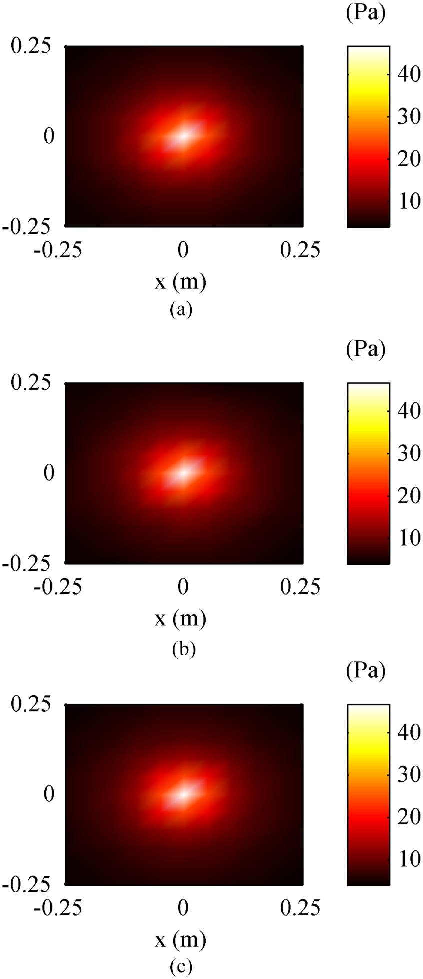
The reconstructed and theoretical pressures at 1000 Hz: (a) theoretical value, (b) obtained by using CESM-p-60, and (c) obtained by using CESM-v-60. (60 means the number of sampling points).
To demonstrate the superiority of CESM-v in sound pressure reconstruction more clearly, Figure 11 gives the reconstruction errors of pressure versus the frequency by using the four models, ESM-p-121, ESM-v-121, CESM-p-60, CESM-v-60. It can be easily seen that all the errors are small and acceptable, even for the maximum error, ESM-p-121, it is less than 13%. And the errors of CESM are smaller, less than 4%. Once again, it is verified that the CESM model performs better than the conventional ESM model in sound pressure reconstruction. At the same time, the models based on the particle velocity measurement are also proved to be superior to the models based on the pressure measurement.
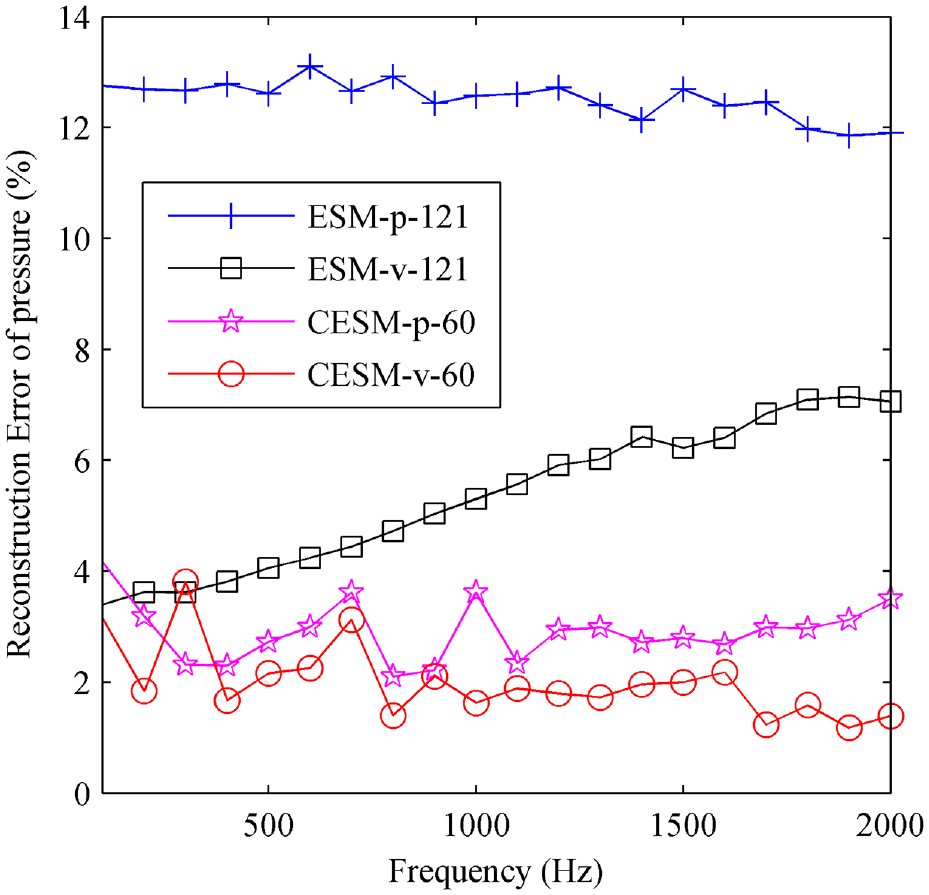
The reconstruction errors of pressure versus frequency by using four models, ESM-p-121, ESM-v-121, CESM-p-60, and CESM-v-60.
Consequently, the proposed CESM-v model performs very well when the sound pressure is to be reconstructed and even better than the CESM-p and the conventional ESM. Being together with the results obtained in Subsection A, all the results presented above illustrate that the proposed CESM-v model can be widely applied in sound field reconstruction no matter the sound pressure or particle velocity is to be reconstructed.
Analysis of parameters in the reconstruction process
In this subsection, the influence of the SNR and the number of sampling points on the reconstruction results of the proposed CESM-v model is analyzed.
Firstly, setting the Gaussian white noise added into the theoretical normal particle velocity from 10 to 50 dB, the CESM-v with 60 sampling points was used to reconstruct the normal particle velocity and sound pressure at 1000 Hz on the reconstruction surface and the reconstruction errors versus SNR are given in Figure 10. For comparison, the ESM-v with 121 sampling points was also used to realize the reconstruction and the errors are also shown in Figure 12. From the figure, it can be seen that the four reconstruction errors decrease gradually with the increase of SNR. When the SNR is 10 dB, both the pressure and normal particle velocity error of the CESM-v are only about 12%, but the pressure error of the ESM-v is up to 25% and the normal particle velocity error of the ESM-v actually exceeds 60%, which can be interpreted as reconstruction failure. This shows that the ESM-v is sensitive to background noise, reflecting bad anti-noise performance, but proves the strong anti-noise performance of the CESM-v. As the SNR increases to 50 dB, the normal particle velocity and pressure error of the ESM-v decrease to 10% and 2%, respectively, which are very small and acceptable. However, the CESM-v presents smaller error, less than 1%. These illustrate that the CESM-v can provide rather stable and accurate reconstruction results under different SNR.
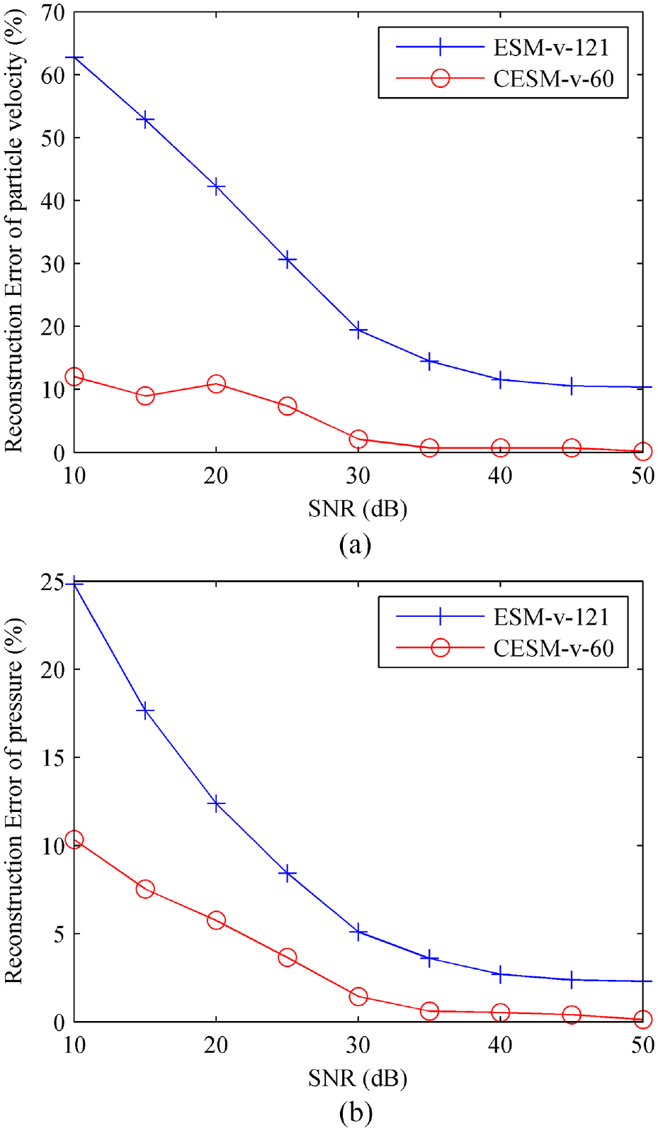
The reconstruction errors versus SNR by using ESM-v-121 and CESM-v-60: (a) the normal particle velocity error and (b) the pressure error.
Secondly, the influence of sampling points on reconstruction results of CESM-v is analyzed. Figure 13 gives the reconstruction errors of normal particle velocity and pressure obtained by using the ESM-v and CESM-v versus the number of sampling points, changing from 40 to 440, corresponding to 10 random sampling arrays. From the figure, it can be found that the normal particle velocity reconstruction error of the ESM-v is more than 50%, and the sound pressure error of the ESM-v is up to 25%. However, the normal particle velocity reconstruction error of the CESM-v is less than 10% and the sound pressure error of the CESM-v is less than 5%. Besides, it can be seen that all the errors decrease with the increase of the number of sampling points, and the reconstruction errors of the CESM-v are always smaller than those of ESM-v. When the number of sampling points reaches 120, the reconstruction errors tend to stability. Observing the reconstruction errors of ESM-v, it can be found that the reconstruction accuracies do not improve significantly as the number of sampling points increases, that is, more sampling points do not make the reconstruction results of ESM-v much better and 120 sampling points is almost enough. But for the CESM-v, 40 sampling points is enough because the errors of both normal particle velocity and sound pressure are always less than 10%. Obviously, the CESM-v can provide much higher reconstruction accuracy with fewer sampling points than ESM-v no matter the normal particle velocity or the sound pressure is to be reconstructed.
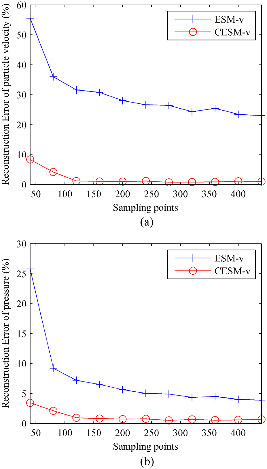
The reconstruction errors versus the number of sampling points by using ESM-v-121 and CESM-v-60: (a) the normal particle velocity error and (b) the pressure error.
Conclusions
In the previous works, the CS theory and the sparse regularization have been applied to the ESM based on the sound pressure measurement by formulating the reconstruction problem in a sparsity framework and this pressure-based CESM, that is, CESM-p model, performs very well in reconstructing the sound pressure. However, the CESM-p model would suffer from the low precision problem in the particle velocity reconstruction as the conventional ESM-p model did. To overcome the problem, this paper proposes a CESM-v model to reconstruct the sound field. In this model, it is the particle velocity instead of the sound pressure that is measured as the input of holographic algorithm to combine with the CS theory and the sparse regularization.
To examine the performance of the proposed CESM-v model, several numerical simulation experiments were carried out.
Firstly, the normal particle velocity was reconstructed by using the proposed CESM-v model as well as the CESM-p model. The results show that the CESM-v overcomes the low precision problem in particle velocity reconstruction, providing much smaller reconstruction errors than the CESM-p. At the same time the conventional ESM with the Tikhonov regularization based on the particle velocity measurement, that is, the ESM-v model, was also used to achieve the reconstructions. What’s an exciting. It is found that the conventional ESM-v even if the measurement is operated on a regular array with sufficient sampling points cannot reach the same level of accuracy of the proposed CESM-v. Furthermore, the reconstruction errors of the normal particle velocity versus the frequency by using the models above are computed and compared. The results show that the proposed CESM-v model performs best, with the reconstruction error less than 11% on the whole frequency band. All in all, the proposed CESM-v model is a meaningful and recommendable method with high accuracy in reconstructing the particle velocity to identify the sound source.
Secondly, the sound pressure was reconstructed by using both the CESM-p and CESM-v models. Analogously, the conventional ESM with the Tikhonov regularization, including the ESM-p and ESM-v models, were also used to reconstruct the sound pressure, and the sound pressure or particle velocity measurement is operated on a regular array with sufficient sampling points. The results show that the CESM models can provide higher reconstruction accuracy than the conventional ESM models, and also verify that the models based on the particle velocity measurement, CESM-v and ESM-v, are superior to the models based on sound pressure measurement, CESM-p and ESM-p. In a word, the proposed CESM-v model performs very well in the sound pressure reconstruction and deserves to be recommended, illustrating the wide applicability of the proposed model.
Thirdly, the influence of the SNR and the number of sampling points on the reconstruction results is studied and analyzed. The results verify once again that the proposed CESM-v model has better performance than the conventional ESM-v model. The CESM-v model has strong anti-noise performance, being able to provide rather stable and accurate reconstruction results under different SNR, and the CESM-v model can provide high reconstruction accuracy with a small number of sampling points.
In conclusion, the proposed CESM-v model is optimal for both the particle velocity and sound pressure reconstruction. On the one hand, the proposed model improves the reconstruction accuracy of the particle velocity when compared to the existing CESM-p model. On the other hand, the proposed model reduces the sampling points much without losing the reconstruction accuracy when compared to the conventional ESM-v. Thus, the proposed CESM-v is a meaningful and recommendable method to reconstruct the sound field, especially in the particle velocity reconstruction.
However, this paper mainly focuses on the simple and compact sound source, and the sound source is assumed in the free sound field environment. For the complicated sound source or the spatially distributed sound sources, or the practical non-free sound field, there are still a lot of work to be done, such as the elaborate construction of the sparse basis,12–14 the application the block SBL, 24 or the elimination of the interference sound source or the reflection of the impedance plane with the sound field separation,26–30,34 when combined with the particle velocity measurement in the future.
Footnotes
Declaration of conflicting interests
The author(s) declared no potential conflicts of interest with respect to the research, authorship, and/or publication of this article.
Funding
The author(s) disclosed receipt of the following financial support for the research, authorship, and/or publication of this article: This work was supported by the National Natural Science Foundation of China [grant numbers 11704110 and 12264015]; and the PhD Research Startup Foundation of East China University of Technology [grant number DHBK2020008].
Data statement
All the data presented in this article have been reported in the manuscript and can be used for the sake of comparison by other researchers. However, the specific computer code used for the computation of the results would remain confidential and would not be shared.