Sage Journals: Discover world-class research

Abstract

Ball screw is widely used in the engineering field, and accurate estimation of their state is crucial for the reliability of system operation. However, existing methods often overlook the time series characteristics and spatial correlation of vibration signals, unable to provide complete degradation information and divide the degradation process, resulting in limited prediction accuracy. Therefore, a state estimation method for ball screw based on Convolutional Neural Networks (CNN) and Long Short-Term Memory Neural Networks (LSTM) is proposed. An experiment of ball screw transmission equipment was conducted to collect vibration signals throughout the entire life cycle and verify the proposed method. Firstly, the frequency domain amplitude signal of the transformed ball screw is normalized to eliminate scale differences, which serves as the input for CNN feature extraction. Then, these deep features are input into the LSTM network to capture the fault evolution patterns that reveal the degradation of ball screw performance, and achieve accurate estimation of ball screw state. The final prediction accuracy was 97.87%, verifying the effectiveness of the proposed method.

Keywords

Ball screw CNN-LSTM neural network performance degradation state estimation

Introduction

The ball screw, a commonly utilized transmission device, plays a pivotal role in the industrial sector. It possesses the attributes of transmitting substantial torque, achieving high precision, and maintaining exceptional stiffness. As a result, it finds extensive application in fields such as machine tools, automation equipment, and aerospace, among others. Nevertheless, owing to the complexity of the working environment and the wear experienced during long-term service, ball screws may succumb to failure and damage, resulting in a decline in equipment performance or even shutdown, which profoundly impacts production efficiency and the economic benefits of enterprises. Consequently, the evaluation of performance and the estimation of the state of the ball screws have emerged as crucial research topics.

Traditional evaluation and prediction methods primarily rely on physical models or empirical formulas. Wen and Gao¹ proposed a model-based RUL prediction method for ball screw systems. Validated by accelerated life test data, the Weighted Mahalanobis Distance (WDMD) demonstrated a significant degradation trend. Zhang et al.² put forth a degradation analysis of ball screws based on wear calculation and a degradation model validated by experimental data. The model’s accuracy and fit were confirmed through cross-validation and failure tests. While these methods offer high accuracy and interpretability, they often depend on a deep understanding of fault mechanisms in practical applications. They are limited by model assumptions and parameter estimations, making it challenging to fully account for complex nonlinear and dynamic changes. To address these limitations, machine learning and deep learning-based approaches have garnered increasing attention from researchers in recent years. By collecting and analyzing sensor data such as vibration, sound, and temperature data from the ball screws, data-driven methods leverage statistical, machine learning, and deep learning algorithms to monitor and predict the performance state of the ball screws. For instance, deep learning algorithms like CNN and LSTM Neural Networks have demonstrated the capability to learn performance patterns from extensive feature data,^3,4 enabling state classification and evaluation. Due to their capacity for automatic learning and nonlinear modeling, these algorithms can capture intricate features and time series evolution patterns, making them widely applicable in the analysis and prediction of vibration time series data.^5–7 To solve the problem that a single health indicator cannot provide complete degradation information and clear division of degradation processes, Xie et al.⁸ introduced a two-stage deep learning model, Attention-ConvFGRNET, for predicting the Remaining Useful Life (RUL) of precision equipment. This model’s performance and effectiveness were verified using the Commercial Modular Aero-Propulsion System Simulation (C-MAPSS) dataset and a ball screw experimental dataset.⁹ Wang et al.¹⁰ proposed an adaptive staged RUL prediction method based on feature fusion. And, two different sets of experiments are carried out to verify the accuracy and superiority of the proposed method in the RUL prediction. The quantity and complexity of environmental parameters such as vibration and temperature collected by sensors can cause non-linear states in the data, making prediction exceptionally difficult. Kundu et al.¹¹ employed Variational Mode Decomposition (VMD) technology to analyze multi-component sensor signals from ball screw drives under narrow bandwidth. Combined with Fisher’s score and Principal Component Analysis (PCA), they predicted RUL, demonstrating the method’s effectiveness on experimental data. Li et al.¹² proposed a systematic ball screw prediction method suitable for fault diagnosis, early diagnosis, health assessment, and RUL prediction. They benchmarked sensor-less and sensor-rich strategies through experiments, showing the method’s effectiveness in implementing Prognostics and Health Management (PHM) analysis. The rapidly developing mechanism and data-driven hybrid integrated network further improve prediction accuracy.¹³ Deng et al.¹⁴ designed a GRU-PF integrated network combining Mixed Particle Filters (PF) and Gated Recurrent Unit (GRU) for ball screw prediction. The method’s effectiveness was confirmed through a ball screw accelerated degradation test (ADT), displaying satisfactory sensitivity prediction. Yang et al.¹⁵ introduced a hybrid RUL prediction architecture, unveiling the precision degradation process of ball screws by introducing clearance as the accuracy index and combining physical and data-driven methods, leading to satisfactory prediction results. Wang et al.¹⁶ proposed a method of RUL prediction of bearing using a fusion network through two-feature cross-weighting (FNT-F), to make up for the shortcomings of feature analysis and achieve complementarity between time-domain and time-frequency features.

While previous studies have made valuable contributions, there remains a need for further research due to the relatively limited number of state estimation studies for ball screws. Existing methods often overlook the time-series nature and spatial correlations of vibrational signals, resulting in limited prediction accuracy. Moreover, there are many methods for estimating the state of bearings, both belong to transmission components and have certain similarities. However, ball screw significantly differs in terms of part units and motion forms, with the characteristics of additional parts and intricate motion forms. Consequently, directly applying bearing state estimation methods to ball screws may not be appropriate. At the same time, the estimation of the operational state of a ball screw may involve complex relationships, such as vibration patterns and variations in workload. The CNN-LSTM network excels in flexibly modeling these intricate relationships by integrating spatial and temporal information, thereby comprehensively capturing the system’s features. Moreover, the CNN architecture demonstrates remarkable performance in feature extraction. Building upon this, leveraging the LSTM network for deeper feature extraction in time-series data and capturing and memorizing long-term dependencies within the system, contributes to a better representation of the system’s state. This is crucial for the comprehensive estimation of the operational state of a ball screw and the enhancement of estimation accuracy. Based on these considerations, the proposed CNN-LSTM model effectively leverages the frequency domain vibration signal of the ball screw. It accentuates frequency domain features, extracts spatial features, and captures temporal features while fully considering the unique characteristics of the ball screws. This model offers a feasible solution for state estimation of ball screws.

Theoretical background

Degradation process of ball screw

The ball screw serves as a prevalent precision motion transmission mechanism employed to convert rotary motion into linear motion. Nevertheless, over time and with alterations in usage conditions, the performance of the ball screw undergoes gradual deterioration and degradation. This process of degradation is intricate and multifaceted, encompassing a multitude of factors and mechanisms. These factors and mechanisms encompass wear, material fatigue, temperature effects,¹⁷ lubricant aging, bending, deformation, and environmental influences.

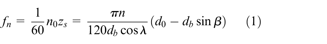
The accumulation of these performance degradation phenomena, as well as the interaction of various factors and mechanisms, will lead to a gradual decline in the performance of the ball screw, ultimately leading to faults mainly caused by severe wear of the ball, severe wear of the screw raceway, and severe wear of the nut raceway, leading to the failure of the ball screw and the inability of the equipment to operate normally. To analyze these phenomena individually, when wear occurs on the nut raceway, it is important to note that the nut is fixed and can be considered a stationary component. In this context, the wear characteristic frequency (f_n) of the nut raceway is equal to the product of the relative rotation frequency of the ball around the lead screw (which is equal to the absolute rotation frequency) and the equivalent number of balls in a single raceway, specifically, as shown in equation (1):

f_{n} = \frac{1}{60} n_{0} z_{s} = \frac{π n}{120 d_{b} \cos λ} (d_{0} - d_{b} \sin β)

(1)

In contrast to the motion of a stationary nut, when wear occurs on the screw raceway, both the ball and the screw move simultaneously in the same direction. In this scenario, the wear characteristic frequency (f_s) of the lead screw raceway is determined by the product of the relative rotation frequency (which is not equal to the absolute rotation frequency) of the ball around the lead screw and the equivalent number of balls in a single raceway. Therefore, the characteristic frequency f_s is associated with the wear of the lead screw is expressed as follows in equation (2):

f_{s} = \frac{1}{60} n_{1} z_{s} = \frac{π n}{120 d_{b} \cos λ} (d_{0} + d_{b} \sin β)

(2)

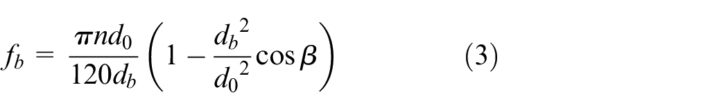
In the case of a ball wear fault, neglecting the influence of the spiral rise angle (γ), the characteristic frequency (f_b) of ball wear can be expressed as follows in equation (3):

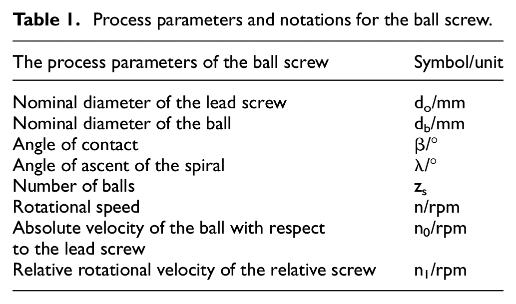
f_{b} = \frac{π n d_{0}}{120 d_{b}} (1 - \frac{{d_{b}}^{2}}{{d_{0}}^{2}} \cos β)

(3)

In summary, the theoretical derivation of the characteristic frequencies for different wear locations in the ball screw has been presented. Specific process parameters and notations for the ball screw used in this paper are provided in Table 1.

Table 1.

Process parameters and notations for the ball screw.

The process parameters of the ball screw	Symbol/unit
Nominal diameter of the lead screw	d_o/mm
Nominal diameter of the ball	d_b/mm
Angle of contact	β/°
Angle of ascent of the spiral	λ/°
Number of balls	z_s
Rotational speed	n/rpm
Absolute velocity of the ball with respect to the lead screw	n₀/rpm
Relative rotational velocity of the relative screw	n₁/rpm

The lifecycle of a ball screw, from initial operation to eventual failure, can be broadly divided into four phases¹⁸: the run-in period, the normal period, the degradation period, and the deterioration period. During the run-in period, minor instabilities may occur due to surface roughness and a lack of adequate adaptation as the surface abrasion defect expands. In the normal period, the ball screw operates smoothly and reliably. As wear becomes noticeable in the degradation period, there is a decrease in transmission accuracy. Finally, during the deterioration period, wear significantly impacts performance, often necessitating extensive repairs or component replacement.¹⁹

In summary, the performance degradation process of a ball screw can be categorized into four distinct phases: the run-in period, the normal period, the degradation period, and the deterioration period. Each of these phases represents varying states and characteristics of the ball screw’s performance degradation. A comprehensive monitoring and understanding of this process, coupled with accurate estimations of its state, holds significant importance. Such insights facilitate timely problem detection and identification, enabling the implementation of appropriate maintenance measures to enhance the reliability of the ball screw, reduce downtime, and minimize production costs.

Convolutional neural networks (CNN)

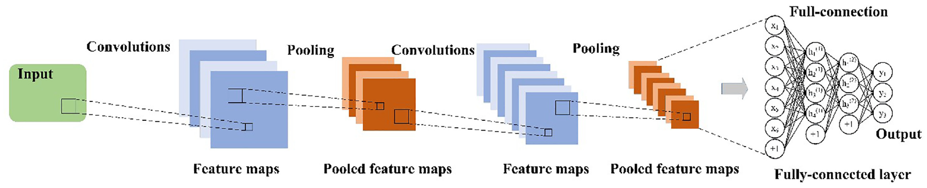
CNN is a deep learning model, the structure of which is illustrated in Figure 1. CNNs are highly effective at extracting features and excel in various feature extraction tasks. The fundamental concept revolves around achieving feature extraction and classification through the efficient integration of convolutional layers, pooling layers, and fully connected layers.^20,21

1) Convolutional Layers: Convolutional layers carry out data conditioning by utilizing learnable filters to extract local features and generate feature maps. The convolution operation can be expressed using the following in equation (4):

Y (i, j) = \sum_{m, n} X (i - m, j - n) \cdot W (m, n) + b

(4)

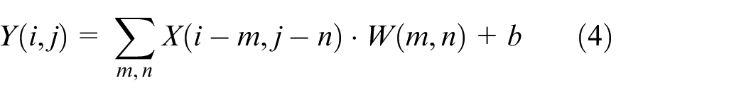
Where Y(i, j) represents a pixel value in the feature map, X(i-m, j-n) represents a pixel value in the input data, W(m, n) represents the weight in the convolution kernel, and b is the bias term. The convolution operation enables the network to extract various features from the input data.

2) Pooling Layer: The pooling layer decreases the spatial dimensions of the feature map while retaining crucial information, accomplishing this through operations such as Max Pooling or Average Pooling.²²

3) Activation Function: An activation function introduces nonlinearity and enhances the network’s capacity to capture intricate features and relationships. Common functions include the Rectified Linear Unit (ReLU), the Exponential Linear Unit (ELU), and the Hyperbolic Tangent (TanH), among others. ELU is a frequently employed nonlinear activation function, and it can be represented by the following in equation (5):

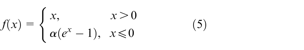
f (x) = {\begin{matrix} x, x > 0 \\ α (e^{x} - 1), x \leq 0 \end{matrix}

(5)

Where x is the input value, α is a constant, which is typically less than 1, controlling the slope of the ELU function in the negative region. The ELU function takes an exponential form in the negative region and is capable of handling negative inputs while preserving some negative information. This nonlinear activation function enhances the network’s ability to learn complex features and nonlinear relationships.

4) Fully Connected Layer: The fully connected layer combines the outputs from the preceding layers to map features to the ultimate output category.

Figure 1.

CNN network structure diagram.

CNNs typically employ cross-entropy loss functions, such as softmax or sigmoid, for classification tasks. However, the sigmoid function is more suitable for prediction tasks.¹⁸ The sigmoid function is represented as follows in equation (6):

f (x) = \frac{1}{1 + e^{- x}}

(6)

In summary, CNNs employ convolutional layers to extract features, pooling layers to reduce dimensionality, activation functions to introduce nonlinearity, and fully connected layers to map features to output categories. This architectural framework allows CNNs to autonomously acquire task-specific features and process extensive datasets efficiently.

Long short-term memory network (LSTM)

LSTM is a type of Recurrent Neural Network (RNN) frequently employed for handling sequential data. It addresses the issue of RNNs lacking long-term memory when processing extended sequences. In contrast to conventional RNNs, LSTMs incorporate gating mechanisms that are more effective at processing lengthy sequences and mitigating the problem of vanishing gradients or exploding gradients.²³

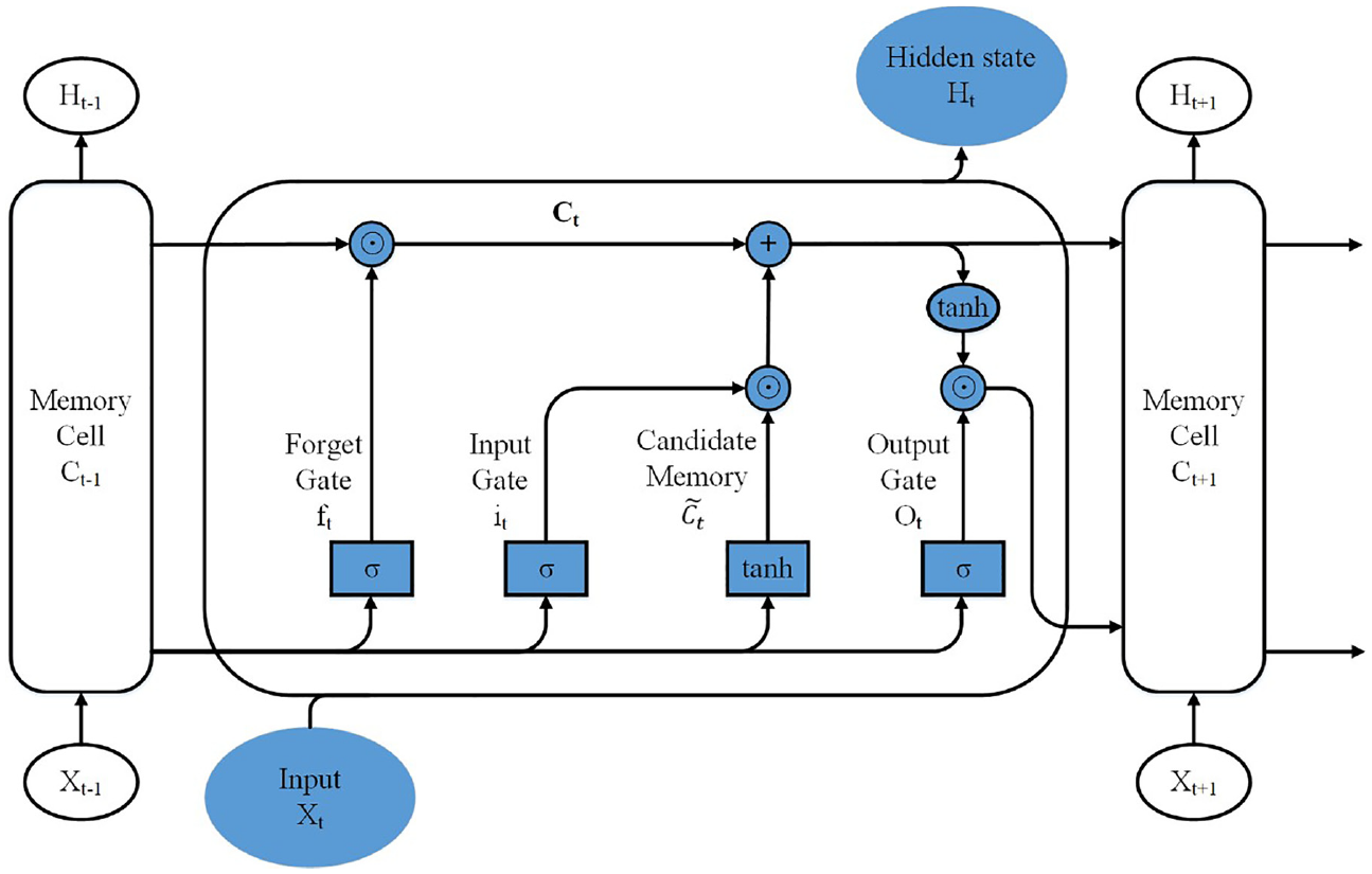
The fundamental component of an LSTM is a cell,^18,24 and its structure is illustrated in Figure 2.

Figure 2.

LSTM cell unit.

An LSTM cell comprises three essential gates: the Forget Gate, the Input Gate, and the Output Gate.²⁵ These gates, along with the Memory Cell and the Gate Unit,²⁶ collectively regulate the flow and storage of information within the LSTM. This architecture enables the LSTM to efficiently manage and leverage previous memories.

1) Memory Cells: Memory cells have the role of storing and updating information over time.

2) Forget Gate: The forget gate determines the extent to which the previous memory cell state should be forgotten. It takes input data and the previous hidden state and produces a value between 0 and 1.²⁷ The formula for the Forget Gate is as follows in equation (7):

f_{t} = σ (W_{f} \cdot [h_{t - 1}, x_{t}] + b_{f})

(7)

Where f_t represents the output of the forgetting gate, W_f denotes the weight matrix of the forgetting gate, h_t-1 stands for the hidden state of the previous time step, x_t signifies the input of the current time step, and b_f represents the bias term of the forgetting gate. These components collectively contribute to the calculation of the Forget Gate in the LSTM cell.

3) Input Gate: The input gate governs the incorporation of new information into the memory cell. It calculates a candidate cell state by considering input data and the previous hidden state. The formula for the Input Gate is as follows in equations (8) and (9):

i_{t} = σ (W_{i} \cdot [h_{t - 1}, x_{t}] + b_{i})

(8)

\tilde{C_{t}} = \tanh (W_{C} \cdot [h_{t - 1}, x_{t}] + b_{C})

(9)

Where i_t represents the output of the input gate, W_i denotes the weight matrix of the input gate, $\tilde{C_{t}}$ signifies the candidate’s new information, W_C represents the weight matrix of the candidate’s new information, b_i and b_C are the bias terms of the input gate and the candidate new information, respectively. These components collectively contribute to the calculation of the Input Gate in the LSTM cell.

4) Updating the Memory Cell: The memory cell is updated by combining the previous cell state with the outputs of the forget gate and the input gate. The formula for updating the memory cell is as follows in equation (10):

C_{t} = f_{t} ⊙ C_{t - 1} + i_{t} ⊙ \tilde{C_{t}}

(10)

Where C_t represents the cell state at the current moment, which corresponds to the memory unit content at the current time step, f_t is the output of the forgetting gate, ⊙ denotes element-wise multiplication, C_t-1 is the cell state at the previous time step, i_t is the output of the input gate, $\tilde{C_{t}}$ is the candidate cell state generated by the input gate. These elements collectively contribute to the calculation for updating the memory cell in the LSTM cell unit.

5) Output Gate: The output gate decides which portions of the memory cell state should be output and generates the final output based on the transformed memory cell state. The formula for the Output Gate is as follows in equations (11) and (12):

O_{t} = σ (W_{O} \cdot [h_{t - 1}, x_{t}] + b_{O})

(11)

h_{t} = O_{t} ⊙ \tanh (C_{t})

(12)

Where O_t represents the output of the output gate, W_O denotes the weight matrix of the output gate,²⁸h_t is the hidden state at the current time step, and b_O stands for the bias term of the output gate.²⁶

These elements collectively contribute to the calculation of the Output Gate in the LSTM cell unit. By integrating the memory unit and gate unit components mentioned above, LSTM empowers the network to make selective decisions about forgetting, incorporating, and outputting information. This capability effectively addresses the issues of gradient vanishing and gradient explosion encountered in traditional RNNs. LSTM achieves the modeling and capture of long-term dependencies within sequential data and possesses robust long-term memory capabilities.

Methods

In this paper, a method for estimating the state of the ball screw, based on the fusion of CNN and LSTM, is proposed. The estimation method consists of two key modules: preprocessing of vibration data and state estimation using the CNN-LSTM network structure.

Vibration signal preprocessing of ball screw

The vibration signal from the ball screw constitutes a crucial data source for evaluating its performance and estimating its state. Nevertheless, the raw vibration signal may contain noise and redundant information that require preprocessing to extract valuable features. Consequently, the Fast Fourier Transform (FFT) is initially applied to the original vibration signal of the ball screw, converting it into a frequency domain representation. Through this transformation, the vibration signal transitions from the time domain to the frequency domain, allowing for the capture of vibration components at various frequencies. The Fast Fourier Transform can be mathematically expressed as follows in equation (13):

X (k) = \sum_{n = 0}^{N - 1} x (n) e^{- j 2 π kn / N}

(13)

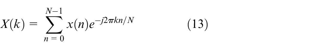
Where X(k) represents the complex value in the frequency domain, x(n) denotes the time domain sampling point in the original vibration signal, N signifies the number of sampling points, and k serves as the index of the sampling point in the frequency domain.

By applying FFT to the original vibration signal, the amplitude spectrum in the frequency domain is obtained. This amplitude spectrum represents the strength of various frequency components within the signal. Through an analysis of the amplitude spectrum, an understanding of the frequency components and energy distribution within the vibration signal of the ball screw is achieved. The frequency domain amplitude data is denoted as the original input.

To mitigate scale variations among different samples and enhance feature robustness, the frequency domain vibration signals obtained from the aforementioned processing undergo normalization. This normalization is a widely adopted data preprocessing technique designed to standardize data with varying dimensions and ranges into a consistent scale range. Common normalization methods include max-min normalization and mean-variance normalization. In this study, max-min normalization is applied to scale and map the amplitude values of the signal within the range of 0–1. The corresponding formula is as follows in equation (14):

x_{norm} = \frac{x - \min (x)}{\max (x) - \min (x)}

(14)

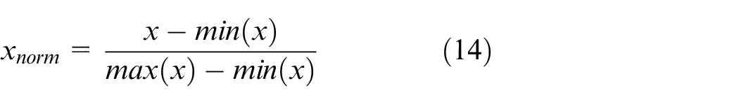
Where x represents the original data, x_norm signifies the normalized data, while min(x) and max(x) denote the minimum and maximum values of the original data, respectively.²⁷

Through normalizing the pre-processed vibration signals in the frequency domain, consistent amplitude ranges for various experimental data can be assured. This guarantees uniform input features for subsequent model training and prediction. Consequently, the potential impact of varying scale ranges on model performance is mitigated, thereby enhancing the stability and accuracy of the subsequent model.

Finally, the dataset is divided into a training set and a test set based on a specific ratio. The training set is used for model training and parameter adjustment, while the test set is employed to evaluate the model’s predictive performance. To mitigate the influence of randomness on experimental results, cross-validation is employed to partition the dataset into multiple subsets. The randperm function is introduced to generate a sequence of non-repeating random integers, as depicted below:

temp = randperm (nwhole)

(15)

Where temp represents the generated sequence of non-repeating random integers, and nwhole represents the first dimension of the dataset, indicating the number of samples. The temp sequence is employed to regulate the extraction of input samples for the CNN-LSTM network, thereby enhancing the model’s generalization capacity.

Construction of the CNN-LSTM network

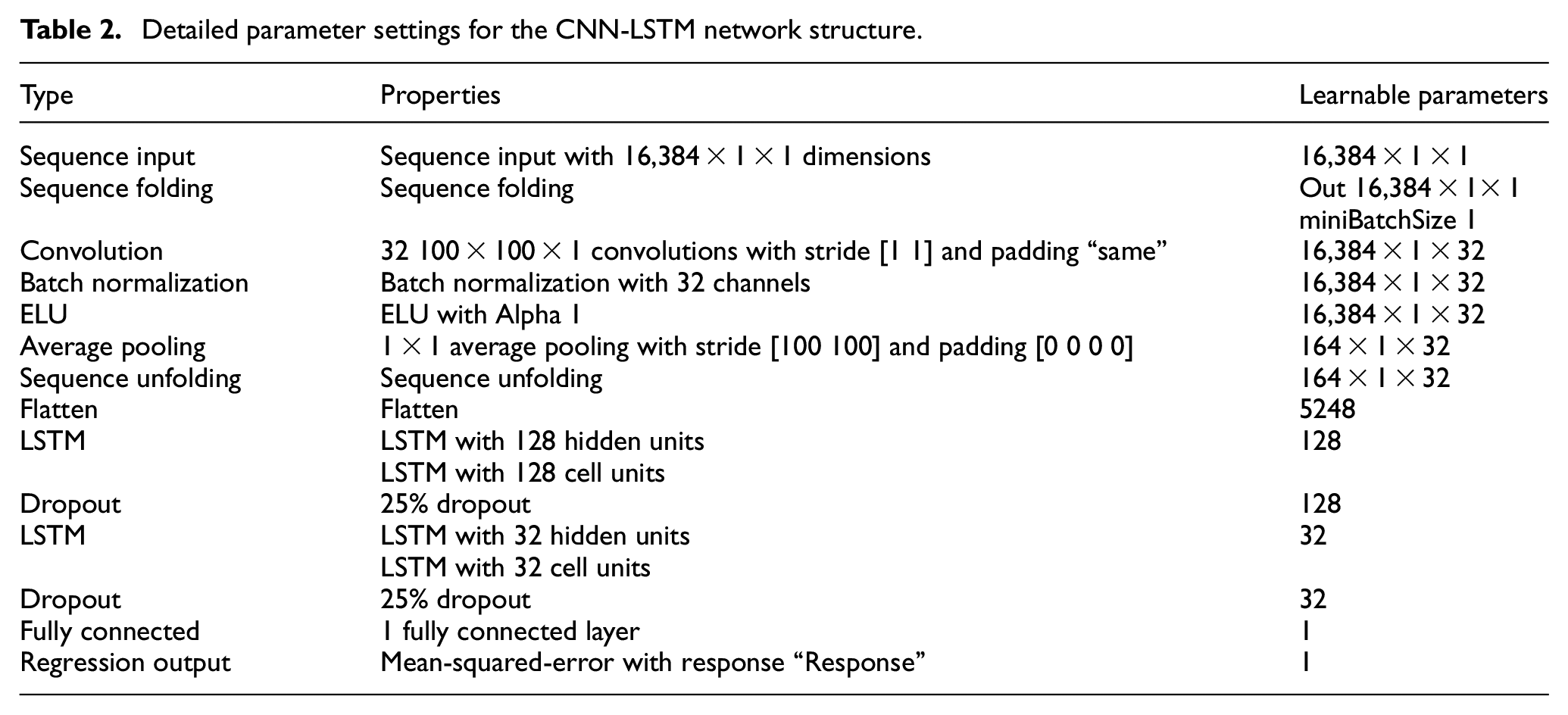
After the original dataset undergoes the preprocessing steps mentioned above, it serves as the input for the CNN, where deep features are extracted and then input into the LSTM network to proceed with ball screw state estimation. Figure 3 illustrates the proposed CNN-LSTM network structure and the process of estimating the state. Detailed parameter settings for the network structure are provided in Table 2. Among them, the first column is the detailed network structure layer, and the second and third columns are the detailed parameter attributes and learnable parameter changes of the corresponding network layer. As shown in Table 2, the input layer and the folding layer are followed by a single-layer convolutional layer.

Figure 3.

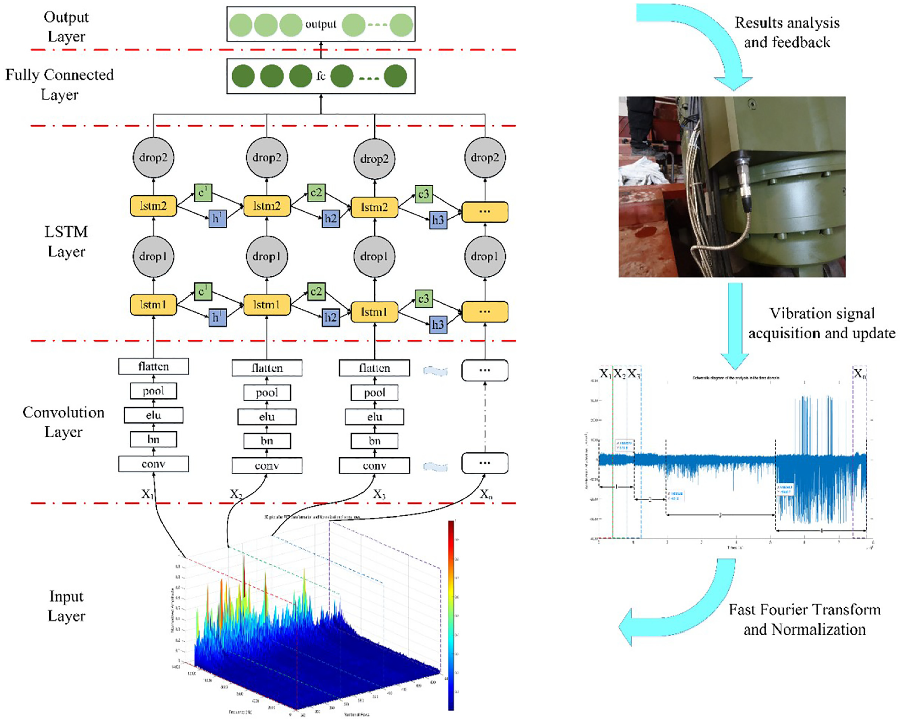
State estimation process for ball screw based on CNN-LSTM neural network.

Table 2.

Detailed parameter settings for the CNN-LSTM network structure.

Type	Properties	Learnable parameters
Sequence input	Sequence input with 16,384 × 1 × 1 dimensions	16,384 × 1 × 1
Sequence folding	Sequence folding	Out 16,384 × 1× 1 miniBatchSize 1
Convolution	32 100 × 100 × 1 convolutions with stride [1 1] and padding “same”	16,384 × 1 × 32
Batch normalization	Batch normalization with 32 channels	16,384 × 1 × 32
ELU	ELU with Alpha 1	16,384 × 1 × 32
Average pooling	1 × 1 average pooling with stride [100 100] and padding [0 0 0 0]	164 × 1 × 32
Sequence unfolding	Sequence unfolding	164 × 1 × 32
Flatten	Flatten	5248
LSTM	LSTM with 128 hidden units LSTM with 128 cell units	128
Dropout	25% dropout	128
LSTM	LSTM with 32 hidden units LSTM with 32 cell units	32
Dropout	25% dropout	32
Fully connected	1 fully connected layer	1
Regression output	Mean-squared-error with response “Response”	1

CNN-LSTM is a deep learning model suitable for processing image and fault data. In the state estimation of the ball screw, the pre-processed frequency domain vibration signal serves as the input for CNN. Key features of the vibration signal are subsequently extracted through parallel convolution layers, batch normalization layers, activation functions, and pooling layers. In CNN’s convolutional layer, convolution kernels of varying sizes are configured to capture features at different scales, thus extracting local patterns from the vibration signals within different frequency ranges. Following the convolutional layer, an activation function is utilized to introduce non-linearity, enabling the neural network to better capture and learn the nonlinear relationships within the data. In this way, the network can more comprehensively represent intricate combinations of various features, thereby enhancing the model’s performance. Pooling layers reduce feature dimensionality through averaging, and retaining the most critical information. By effectively combining smoothing layers, pooling layers, activation function layers, the normalization layers, CNNs gradually learn higher-level abstract features. These features can capture characteristics such as periodicity, frequency variations, and nonlinear changes within the vibration signal of the ball screw. Moreover, CNN offers advantages such as translation invariance and parameter sharing, enabling effective processing of the ball screw’s vibration signal. The deep features extracted by CNN serve as input to the LSTM network, allowing it to capture the fault evolution patterns within the vibration signal.²⁹ LSTM’s gating mechanism enables it to efficiently handle long-term dependencies, making it well-suited for modeling time series data. Additionally, to enhance the network’s generalization capability and improve model robustness,³⁰ a Dropout layer is introduced into the network structure alongside the LSTM layer. Dropout is a regularization technique employed to prevent overfitting. During training, the Dropout layer randomly sets the output of a subset of neurons to zero, reducing inter-neuron dependencies. Through the stacking of multiple LSTM and Dropout layers, the LSTM model is thoroughly trained, progressively learning the trend quantification information embedded within the ball screw’s vibration signal, which reveals the performance evolution trend.

Full life cycle testing and data analysis

Full life cycle testing design of ball screw

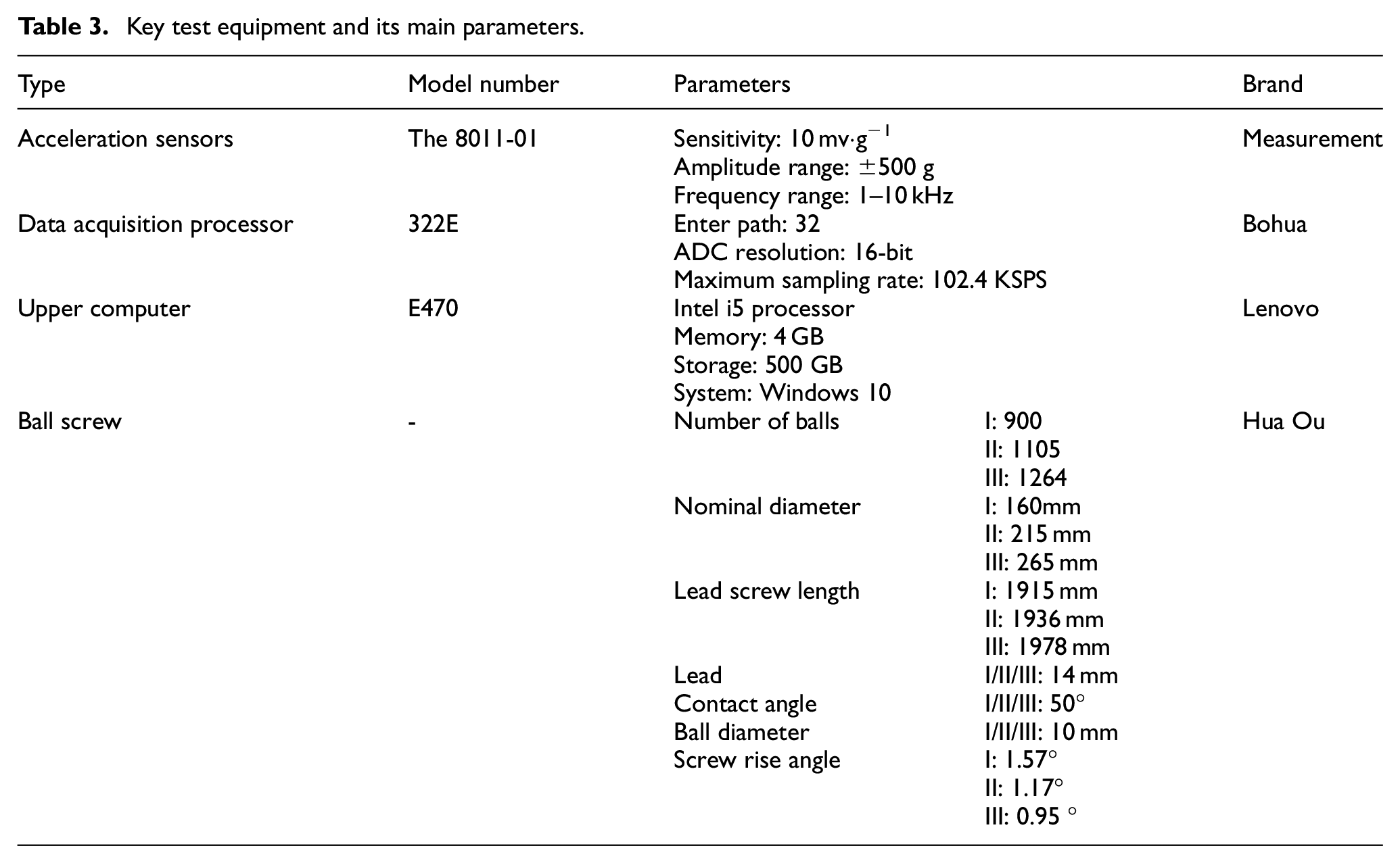
To validate the effectiveness of the proposed method, an experimental test platform was constructed to investigate the degradation behavior of the ball screw. The experimental test platform comprises a three-stage (I/II/III) ball screw drive system used in a specific type of vehicle. In this experimental test platform, the I-stage screw is driven by four servo motors operating at a speed of 6200 RPM. The motor speeds are adjusted using a gearbox in the reducer, transmitting motion to the II and III-stage screws, which, in turn, drive the entire ball screw to facilitate load movement. An acceleration sensor is mounted atop the screw using a specialized sensor base, and the raw vibration signal is transmitted to the data acquisition processor via a dedicated cable for preprocessing. The lifetime test of the ball screw system was conducted for a total of 6000 operating cycles, equivalent to 6000 extension and retraction of lead screws, with a sampling time of 0.64 s and a sampling frequency of 25.6 kHz. Each vibration acquisition sample consisted of 16,384 sampling points. The results are displayed on the host computer. The testing period began on May 6, 2022, and concluded on May 11, 2023, spanning approximately 1 year. During this time, lubrication was replenished and maintained a total of 13 times. The configuration of the test bench is illustrated in Figure 4 below. Detailed parameters of the key hardware equipment used during the test are presented in Table 3.

Figure 4.

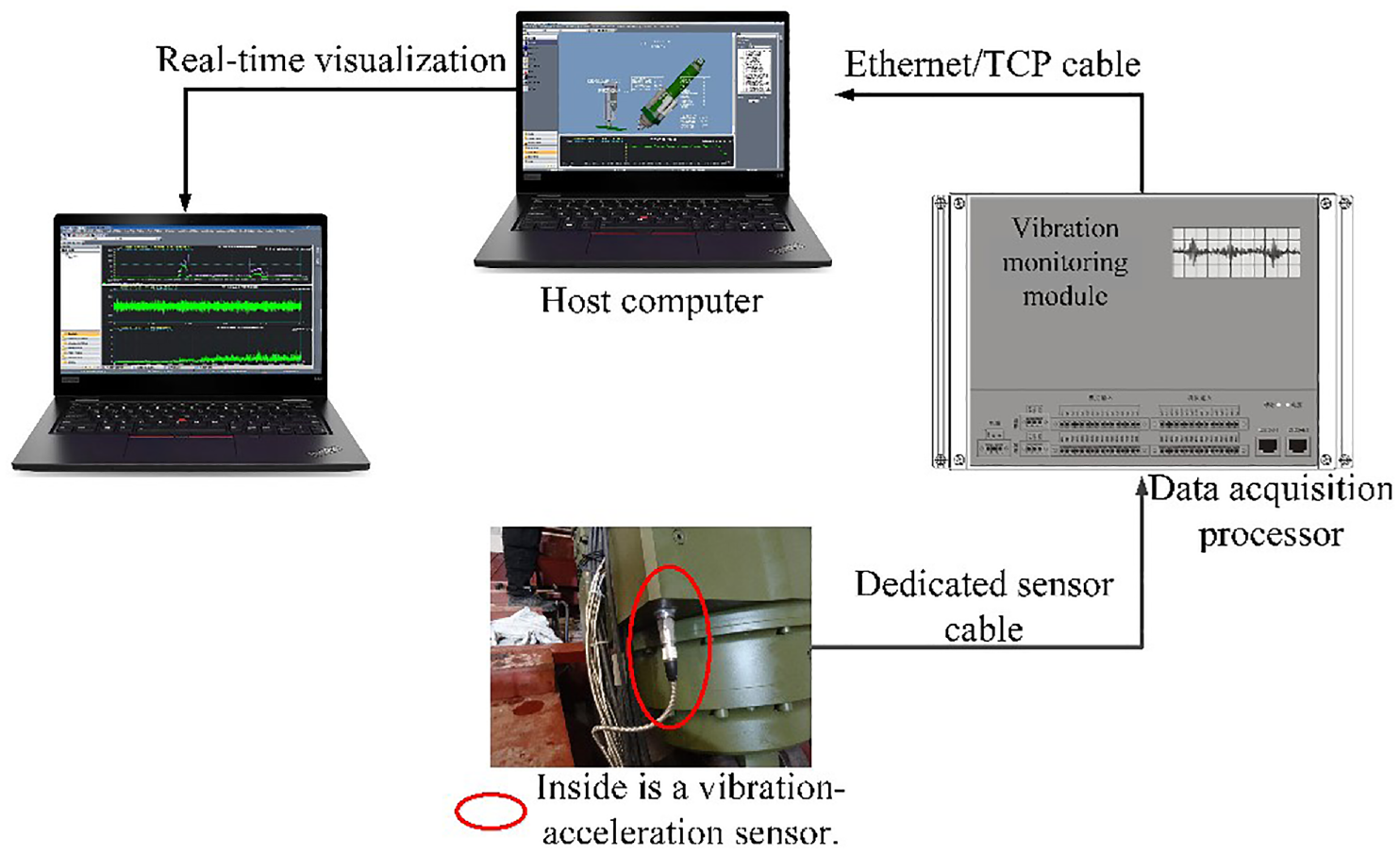
Structure diagram of the test bench.

Table 3.

Key test equipment and its main parameters.

Type	Model number	Parameters		Brand
Acceleration sensors	The 8011-01	Sensitivity: 10 mv·g⁻¹ Amplitude range: ±500 g Frequency range: 1–10 kHz		Measurement
Data acquisition processor	322E	Enter path: 32 ADC resolution: 16-bit Maximum sampling rate: 102.4 KSPS		Bohua
Upper computer	E470	Intel i5 processor Memory: 4 GB Storage: 500 GB System: Windows 10		Lenovo
Ball screw	-	Number of balls	I: 900	Hua Ou
			II: 1105
			III: 1264
		Nominal diameter	I: 160mm
			II: 215 mm
			III: 265 mm
		Lead screw length	I: 1915 mm
			II: 1936 mm
			III: 1978 mm
		Lead	I/II/III: 14 mm
		Contact angle	I/II/III: 50°
		Ball diameter	I/II/III: 10 mm
		Screw rise angle	I: 1.57°
			II: 1.17°
			III: 0.95 °

Data analysis

Time-frequency analysis

By synchronizing the collected vibration data with the motor speed data, time-domain plots of speed and vibration were obtained. These plots enabled the comparison of vibration changes under the same working conditions (load and speed) at different test times. Figure 5 displays the time-domain plots of vibrations and speeds for selected test epochs. In each of the three graphs in Figure 5, (a) is the normal operating period, (b) is the degradation period, (c) is the deterioration period, the red lines represent rotational speed data for the entire test duration, while the blue lines depict vibration data for the same duration.

Figure 5.

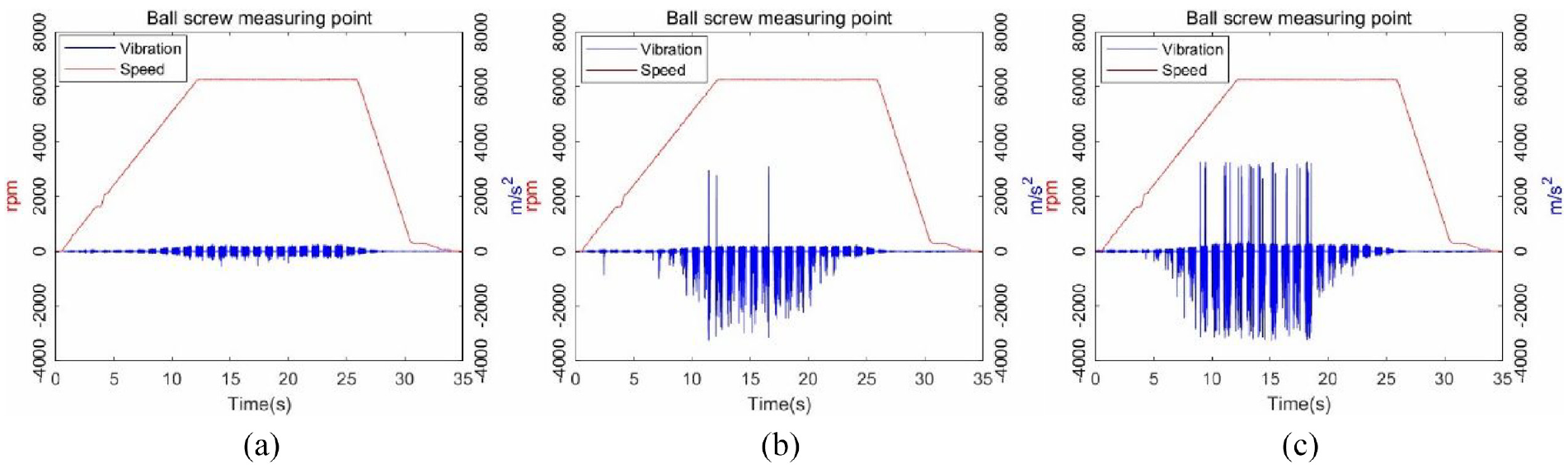
Time-domain plots of vibration and rotational speed for some test times: (a) the normal operating period; (b) the degradation periods and (c) the deterioration period.

After obtaining the time-domain signal through data sorting, a Fourier transform is performed to obtain the frequency-domain signal. Based on the vibration change trends observed in the time-domain signal, the equipment’s operating state is analyzed to assess whether deterioration has occurred. By comparing the changes in different characteristic frequencies, the presence of any faults is determined. Figure 6 illustrates a schematic diagram of the frequency-domain analysis corresponding to the time-domain plots of vibrations and speeds for the specified test epoch.

Figure 6.

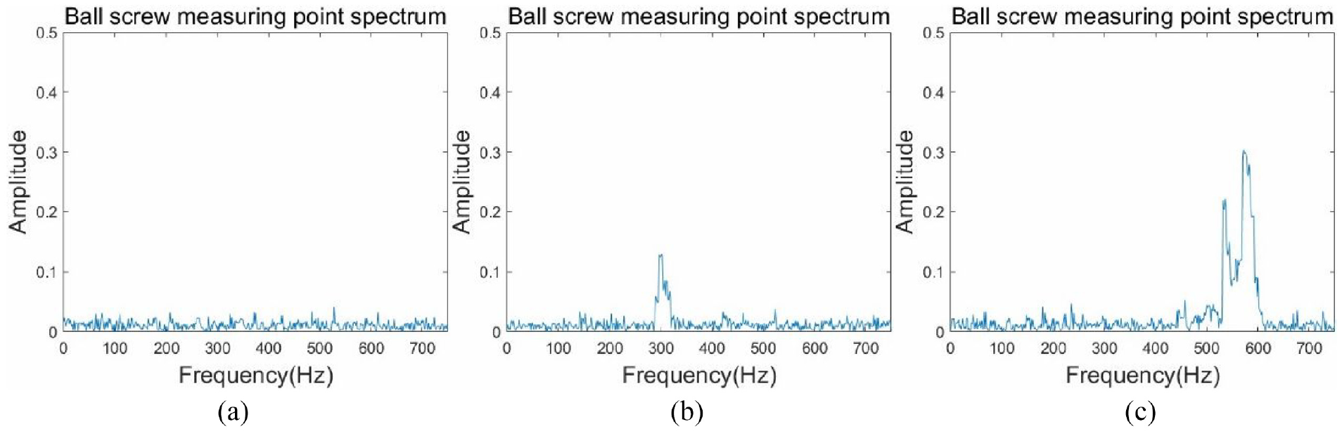
Schematic diagram of the frequency domain analysis corresponding to the above time domain diagram of vibration and speed: (a) the normal operating period; (b) the degradation period and (c) the deterioration period.

As the service time of the ball screw increases, the degree of wear gradually intensifies, leading to issues such as abnormal noise and vibration. These issues are reflected in the time-domain diagram, where the vibration acceleration values change from small to large and from sparse to dense, as illustrated in Figure 5. This phenomenon is further analyzed in the frequency domain, where an increase in the amplitude occurs at specific frequencies, along with a shift in the frequency amplitude spike transfer among different frequency domain plots. Time-domain variations are utilized to assess whether the equipment’s operation is deteriorating, while frequency-domain variations are employed to determine the presence of equipment failures.

Trend change analysis

The results of the aforementioned analysis of time- and frequency-domain variations manifest at the fault mechanism level of the ball screw. Utilizing the theory and model algorithm (as outlined in Table 4 below), the characteristic frequency of the target fault in the ball screw is computed and analyzed. Observing changes in the characteristic frequency serves to reflect fault symptoms and identify the fault mode of the ball screw.

Table 4.

Ball screw equipment fault locating target and diagnosis method.

Diagnose locate the target	Fault mode	Detailed diagnostic design
Ball	(I/II/III) The ball is seriously worn.	$f_{b} = \frac{π n d_{0}}{120 d_{b}} (1 - \frac{{d_{b}}^{2}}{{d_{0}}^{2}} \cos β)$
Lead screw raceway	(I/II /III) The lead screw raceway is seriously worn.	$f_{s} = \frac{1}{60} n_{1} z_{s}$ $= \frac{π n}{120 d_{b} \cos λ} (d_{0} + d_{b} \sin β)$
Nut raceway	(I/II/III) The nut raceway is seriously worn.	$f_{n} = \frac{1}{60} n_{0} z_{s}$ $= \frac{π n}{120 d_{b} \cos λ} (d_{0} - d_{b} \sin β)$

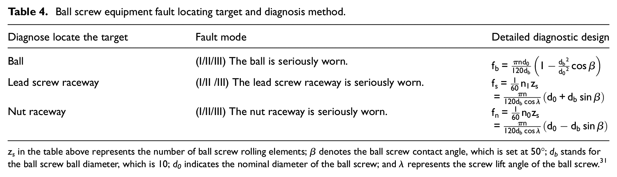
z_s in the table above represents the number of ball screw rolling elements; β denotes the ball screw contact angle, which is set at 50°; d_b stands for the ball screw ball diameter, which is 10; d₀ indicates the nominal diameter of the ball screw; and λ represents the screw lift angle of the ball screw.³¹

By employing the algorithm described above, the characteristic frequency of the key transmission equipment within the ball screw can be derived. The characteristic frequency amplitudes under various test conditions are connected to create a chart illustrating the trend of characteristic frequency changes. This chart is instrumental in comparing the equipment’s operational state variations. Fault diagnosis is conducted by contrasting the changes in vibration characteristic frequency amplitudes between normal and faulty conditions.

The ball screw exhibits varying vibrational properties during different operational phases. In the initial operation stage, due to inadequate lubrication of the ball screw system, it may exhibit some slightly unstable operating characteristics. The normal period represents a phase of stable operation for the ball screw. By this stage, operating conditions have been adapted, surface smoothness of components like balls, screws, and guide rails has improved, their contact and cooperation have become better suited, and wear levels are relatively low. As the ball screw undergoes long-term use and experiences changing usage conditions, signs of wear become evident during the degradation phase. The wear on the ball’s surface, lead screw’s surface, and guide rail’s surface gradually increase, leading to reduced transmission accuracy and increased friction. Finally, the ball screw enters a deterioration phase, characterized by severe wear that significantly impacts performance, rendering it incapable of meeting design requirements. During this phase, the ball screw may exhibit issues such as abnormal noise, vibration, increased transmission errors, and even complete failure. Hence, it is appropriate to select data for analysis from both the degradation and non-degradation periods to observe changes in the amplitude of vibrational characteristic frequencies. While using extensive data can better represent the actual operational conditions, it can also place a significant burden on data processing and increase time consumption. Based on the above considerations, it has been decided to extract an appropriate amount of data from the 3260 to 5660th trial, which is in the degradation and deterioration stages, for analysis, with every 100 trials as the span. The final frequency amplitude variation obtained is shown in Figure 7.

Figure 7.

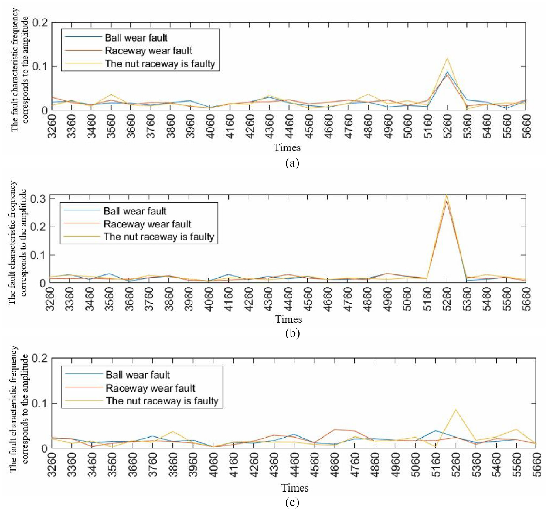
Trend graph of frequency amplitude variation for some experimental times: (a) corresponding amplitude of the characteristic frequency of a First-stage screw fault, (b) corresponding amplitude of the characteristic frequency of a second-stage screw fault, and (c) corresponding amplitude of the characteristic frequency of a three-stage screw fault.

State estimation

Division of life cycle stages (label establishment)

Collect vibration data of the entire life cycle of the ball screw, and use it as a basis to construct labels to cooperate with network training. To categorize the life cycle into four stages, three critical points needed determination: the onset of the normal period,^18,32 the onset of the performance degradation stage, and the boundary between the performance degradation period and the deterioration period. Theoretically, the time-domain vibration acceleration values exhibit different distributions across various stages. Therefore, this paper will establish network training labels based on the division of the life cycle stages.

After conducting a total of 6000 tests on the ball screw, considering the substantial volume of data and the minimal fluctuation in vibration acceleration values between adjacent test instances, one set of vibration acceleration data was collected every 10 tests from the overall dataset. Furthermore, due to the potential for errors or incomplete data during the acquisition process, certain data points needed to be discarded. Consequently, 477 sets of complete vibration acceleration data were successfully obtained.

To facilitate a comprehensive understanding and analysis of the collected data, the 477 sets of experimental data were reorganized sequentially from 1 to 477, aligning with the order of experiments. This reordering enables us to treat the obtained data series as the vibration acceleration data of the ball screw throughout its complete life cycle. Upon performing a time-domain analysis of these data, it became evident that the data could be distinctly categorized into four stages. Depending on the number of labeled sampling points, which correspond to the X-coordinate values and given the collection of 16,384 sampling points in each epoch, these four stages were transformed into respective test epochs ranging from 1 to 64 (the run-in period: tests 1–1795 constitute the first stage, with tests 1165–1795 selected for research to manage data volume); 65–106 (normal period: tests 1805–2215 are the second stage); 107–314 (degradation period: tests 2225–4370 constitute the third stage, with tests 2225–3145 and 3230–4370 selected for research, considering the large volume of data and the significance of the degradation period for guiding state estimation); and 315–477 (deterioration period: tests 4380–6000 are the fourth stage). The corresponding time-domain analytical plots are presented in Figure 8.

Figure 8.

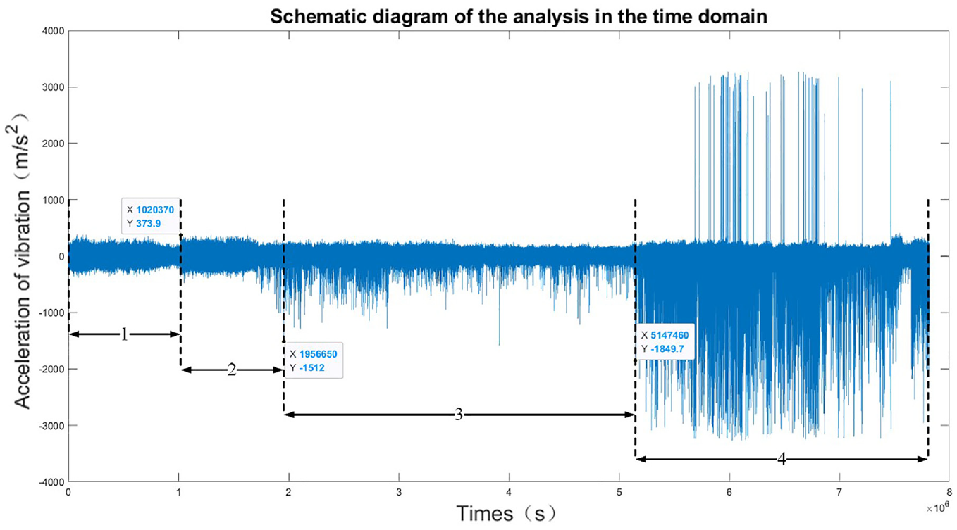
Time domain diagram of the full life cycle of the ball screw.

Based on this observation, the starting point of the normal period, the starting point of the performance degradation stage,¹⁸ and the dividing point between the performance degradation period and the deterioration period in the performance degradation process of the ball screw were determined. These points correspond to the 65th, 107th, and 315th tests, respectively. These four stages align with the performance degradation stages of the ball screw described in section 2.1 above. Specifically: the first stage, comprising tests 1–64, is designated as the running-in period; the second stage, encompassing tests 65–106, is labeled as the normal period; the third stage, consisting of tests 107–314, is denoted as the degradation period; and the final stage, which includes tests 315–477, is termed the deterioration period.

Once the life cycle stages of the ball screw have been divided, the label construction process is initiated. Each stage is assigned a corresponding label value: 1 for the running-in period, 2 for the normal period, 3 for the degradation period, and 4 for the deterioration period. This association effectively links the vibration acceleration data with the distinct performance degradation stages of the ball screw, providing a labeled basis for further research into the performance changes of the ball screw. This labeling scheme aids in subsequent performance analysis and prediction efforts. The constructed labels are displayed in Figure 9:

Figure 9.

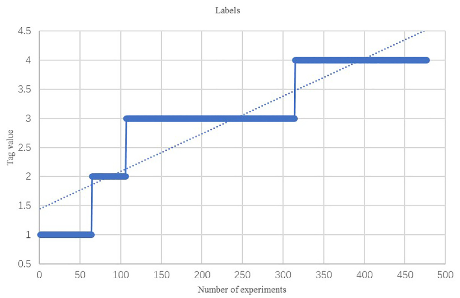
The constructed label graph.

Network training process

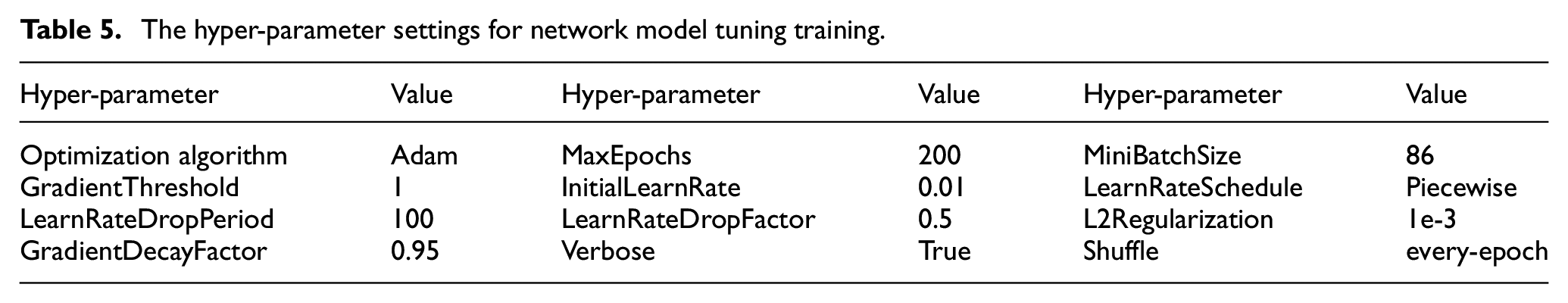
After completing the construction of the CNN-LSTM network structure and the establishment of corresponding labels, the subsequent training and parameter optimization of the network can commence. The training process is depicted in Figure 10 below. The dataset was divided into 430 training sets and 47 test sets at a ratio of 0.901:0.099. During network training, the Adam optimization algorithm is employed to minimize the loss function and adjust the parameters of the CNN and LSTM models. A gradient threshold of 1 is set, and if the network’s gradient surpasses this threshold, it will be truncated or scaled. The dataset is shuffled at the start of each training cycle to enhance sample randomness and generalization. A gradient decay factor of 0.95 is specified to regulate the gradient’s decay rate, thereby enhancing training stability and convergence. To control model complexity and mitigate overfitting, L2 regularization, and an early stopping strategy are employed during network training. The hyperparameter configurations for tuning the network model during training are presented in Table 5.

Figure 10.

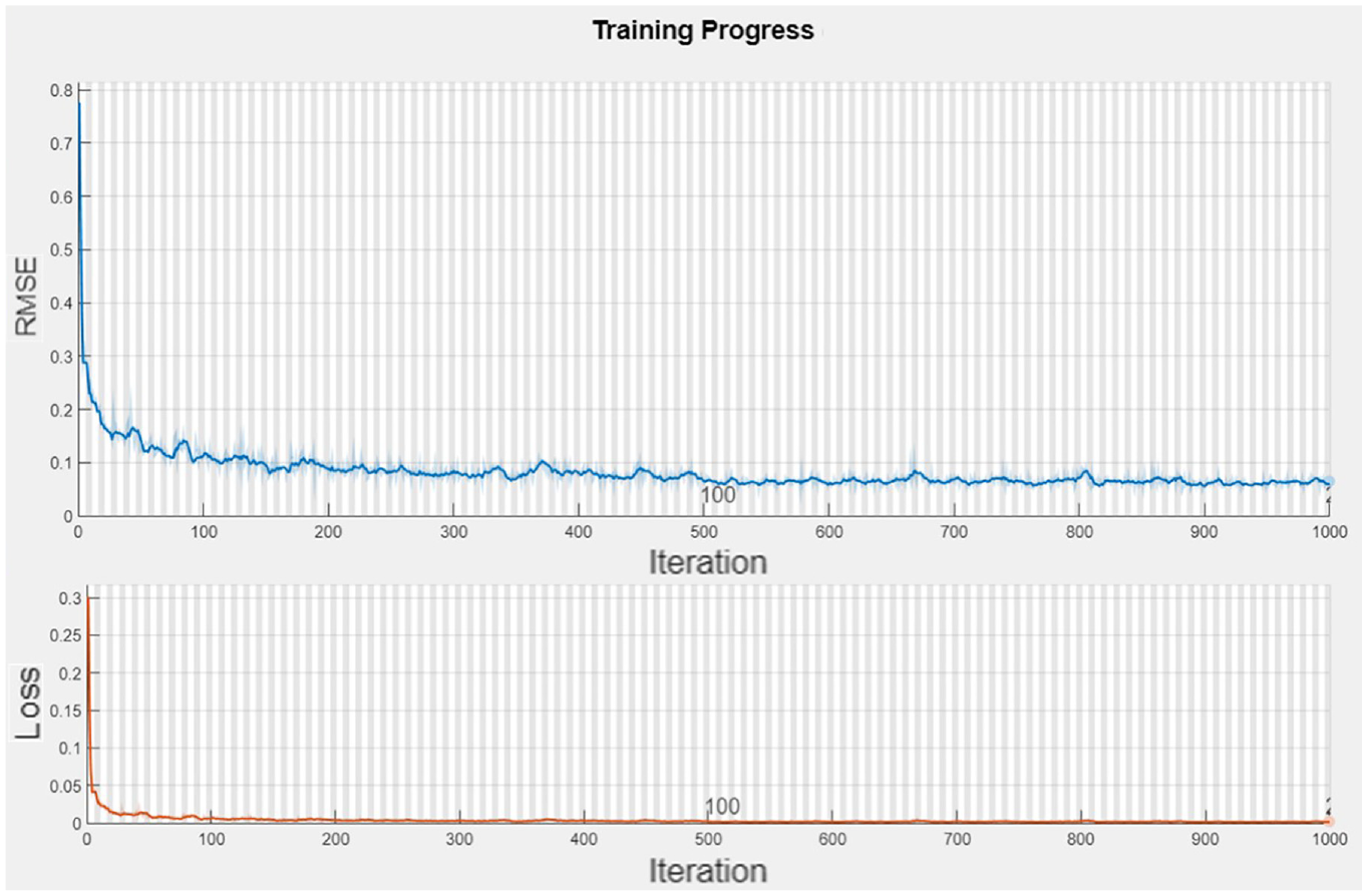
CNN-LSTM network training progress and parameter settings.

Table 5.

The hyper-parameter settings for network model tuning training.

Hyper-parameter	Value	Hyper-parameter	Value	Hyper-parameter	Value
Optimization algorithm	Adam	MaxEpochs	200	MiniBatchSize	86
GradientThreshold	1	InitialLearnRate	0.01	LearnRateSchedule	Piecewise
LearnRateDropPeriod	100	LearnRateDropFactor	0.5	L2Regularization	1e-3
GradientDecayFactor	0.95	Verbose	True	Shuffle	every-epoch

The trained CNN-LSTM model is utilized for estimating the state of the ball screw. By inputting the current vibration signal, the model generates an estimation of the ball screw’s state, thereby enabling timely monitoring of the ball screw’s performance status. This, in turn, facilitates proactive maintenance or replacement measures, optimization of production planning, and reduction of maintenance costs.

Analysis of prediction results

After the life test of the ball screw was completed, 477 complete sets of data were successfully obtained as shown in Figure 8. This data sequence is considered the vibration acceleration data within the complete life cycle of the ball screw.³³ However, it is essential to acknowledge that an excessively large sample dataset could potentially impact the training and performance of the CNN-LSTM network.³⁴ Large datasets often require more powerful hardware for training, including larger storage capacity and higher computational speed, leading to increased training costs. Simultaneously, the network needs to handle more samples, resulting in a more time-consuming training process. Particularly in situations with limited resources, it generally necessitates greater computational resources and additional training iterations. Ensuring the quality of data during the processing of large datasets is also a challenge. With the expansion of the dataset, more complex models are required. However, overly complex models may lead to overfitting and a decline in generalization performance. Additionally, when dealing with large datasets, there is a higher risk of the model overfitting the training data, potentially requiring stronger regularization strategies to ensure the quality and balance of the dataset.

To address these issues, a selective approach was employed where the complete vibration acceleration data from each test was strategically intercepted. Specifically, data collected during periods of steady-state speed were chosen to create a new dataset, which was subsequently used as input samples for prediction. This approach offers several advantages: Firstly, by selectively extracting key samples, reducing the scale of training data, and minimizing the required storage space, data management becomes more efficient. Simultaneously, using a more streamlined dataset enhances computational efficiency, shortens training time, and allows the model to converge to the optimal solution more quickly. This contributes to expediting the training process, especially in scenarios with limited computational resources. Secondly, In the process of selectively extracting data, the focus is on data representing the stable operational state of the equipment, ensuring data quality. This aids the model in better learning useful features without being affected by noise or instability. Choosing only representative samples with critical information enhances the model’s generalization capability, reducing the risk of overfitting the training data. Furthermore, training the model on more representative and interpretable samples contributes to understanding the model’s decision-making process, enhancing model interpretability.

After training with 430 sets of training samples, the network made predictions on 47 sets of test set data. The prediction results generated by the CNN-LSTM network are illustrated in Figure 11(a) below. Additionally, LSTM and CNN networks were configured to make separate predictions, providing a basis for comparison, and the outcomes are presented in Figure 11(b) and (c) below.

Figure 11.

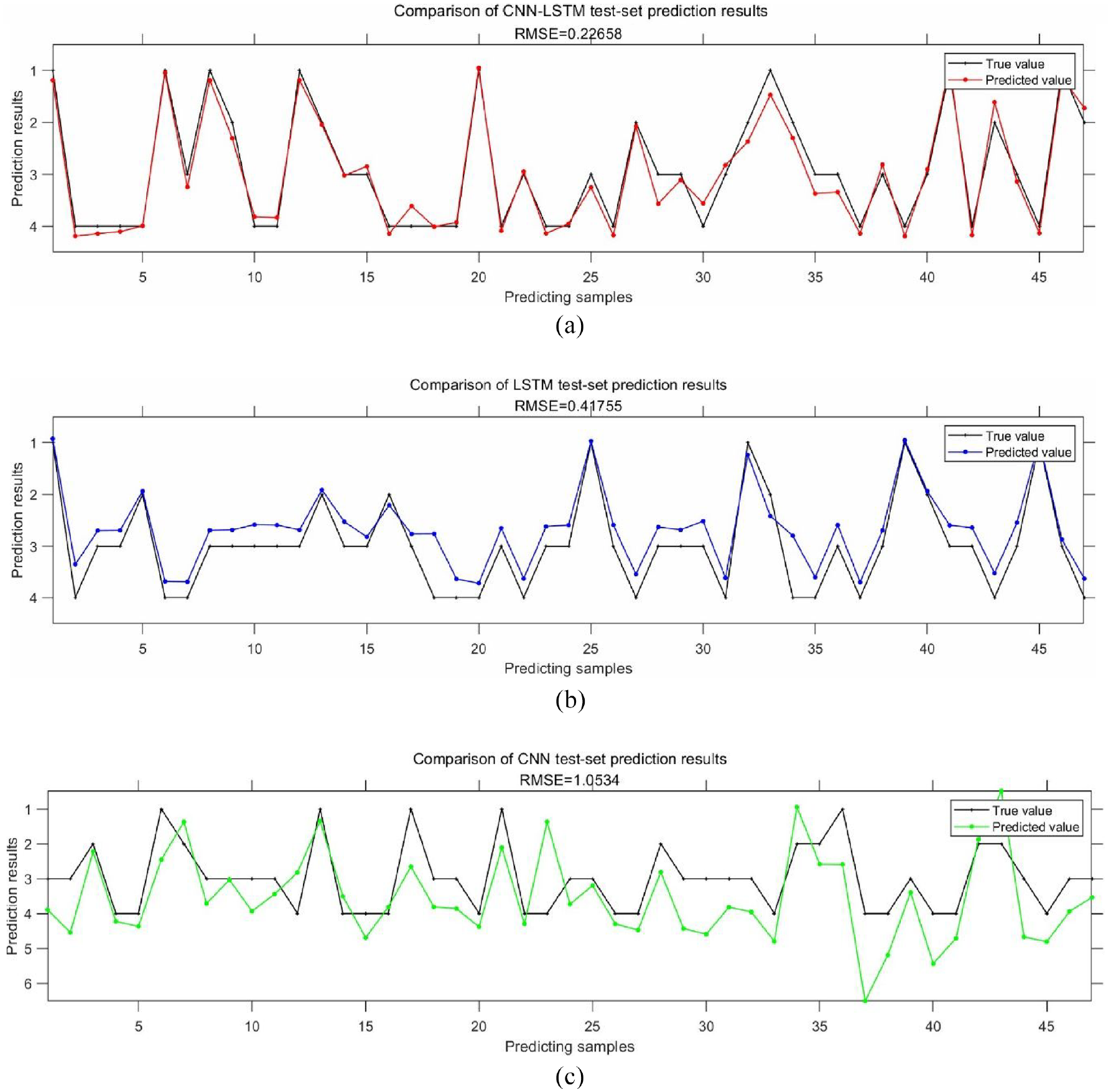
Schematic diagram of the prediction results: (a) CNN-LSTM prediction results, (b) LSTM prediction results, and (c) CNN prediction results.

As depicted in the analysis presented in Figure 11, it is evident that the predictions of the CNN-LSTM structure are in better agreement with the actual values among the three network structures, with LSTM having the second-best performance and CNN displaying the least favorable predictive accuracy. Furthermore, the prediction performance of LSTM is significantly improved compared to CNN, which is consistent with the suitability of LSTM networks for processing time series data.

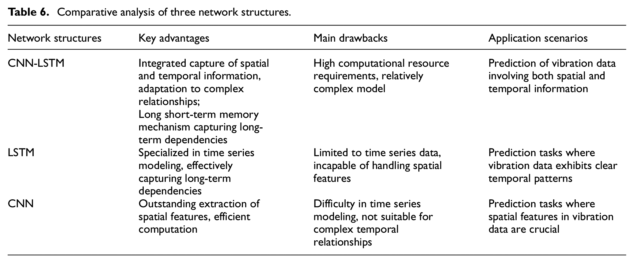
Table 6 summarizes the primary strengths and weaknesses of each network structure, along with their applicability in various types of data prediction scenarios, providing an intuitive representation of their relative performance. Analysis from Table 6 indicates that the CNN-LSTM structure exhibits broader applicability compared to the CNN and LSTM structures, making it more suitable for handling complex relationships. The LSTM structure, in contrast to the CNN structure, excels in processing sequences with clear temporal characteristics. The CNN structure is better suited for predictive tasks where spatial features in the data are more critical.³⁵ This aligns with the experimental results of processing time-series vibration data from ball screws: the CNN-LSTM structure demonstrated the highest prediction accuracy, followed by the LSTM structure, and the CNN structure exhibited the lowest accuracy.

Table 6.

Comparative analysis of three network structures.

Network structures	Key advantages	Main drawbacks	Application scenarios
CNN-LSTM	Integrated capture of spatial and temporal information, adaptation to complex relationships; Long short-term memory mechanism capturing long-term dependencies	High computational resource requirements, relatively complex model	Prediction of vibration data involving both spatial and temporal information
LSTM	Specialized in time series modeling, effectively capturing long-term dependencies	Limited to time series data, incapable of handling spatial features	Prediction tasks where vibration data exhibits clear temporal patterns
CNN	Outstanding extraction of spatial features, efficient computation	Difficulty in time series modeling, not suitable for complex temporal relationships	Prediction tasks where spatial features in vibration data are crucial

To visually illustrate the accuracy and precision of the CNN-LSTM model for estimating the state of a ball screw, an in-depth analysis of the distribution of the prediction results is conducted, ranging from a minimum of 0.9051 to a maximum of 4.1943. Furthermore, some values, such as 2.3534 and 2.7314, which deviate significantly from the nominal values 2 and 3, are observed but do not strictly align with intermediate values like 2.5. To attribute such predicted values appropriately, an adequate classification criterion is required to ensure comprehensive coverage of all predicted results and equal weighting for each predicted value. Taking the above factors into consideration, the current state is categorized as follows based on predicted values: If the predicted value falls between 0.5 and 1.5, the current state is considered to be in the run-in period. If the predicted value falls between 1.5 and 2.5, the current state is regarded as normal. If the predicted value falls between 2.5 and 3.5, the current state is deemed to be in the degradation phase. If the predicted value falls between 3.5 and 4.5, this criterion identifies the current state as a deterioration period. The predictions are subject to statistical analysis and comparison with true values. The statistical results are presented in bar Figure 12(a) as follows. Similarly, the statistical results for LSTM and CNN are displayed in Figure 12(b) and (c), respectively.

Figure 12.

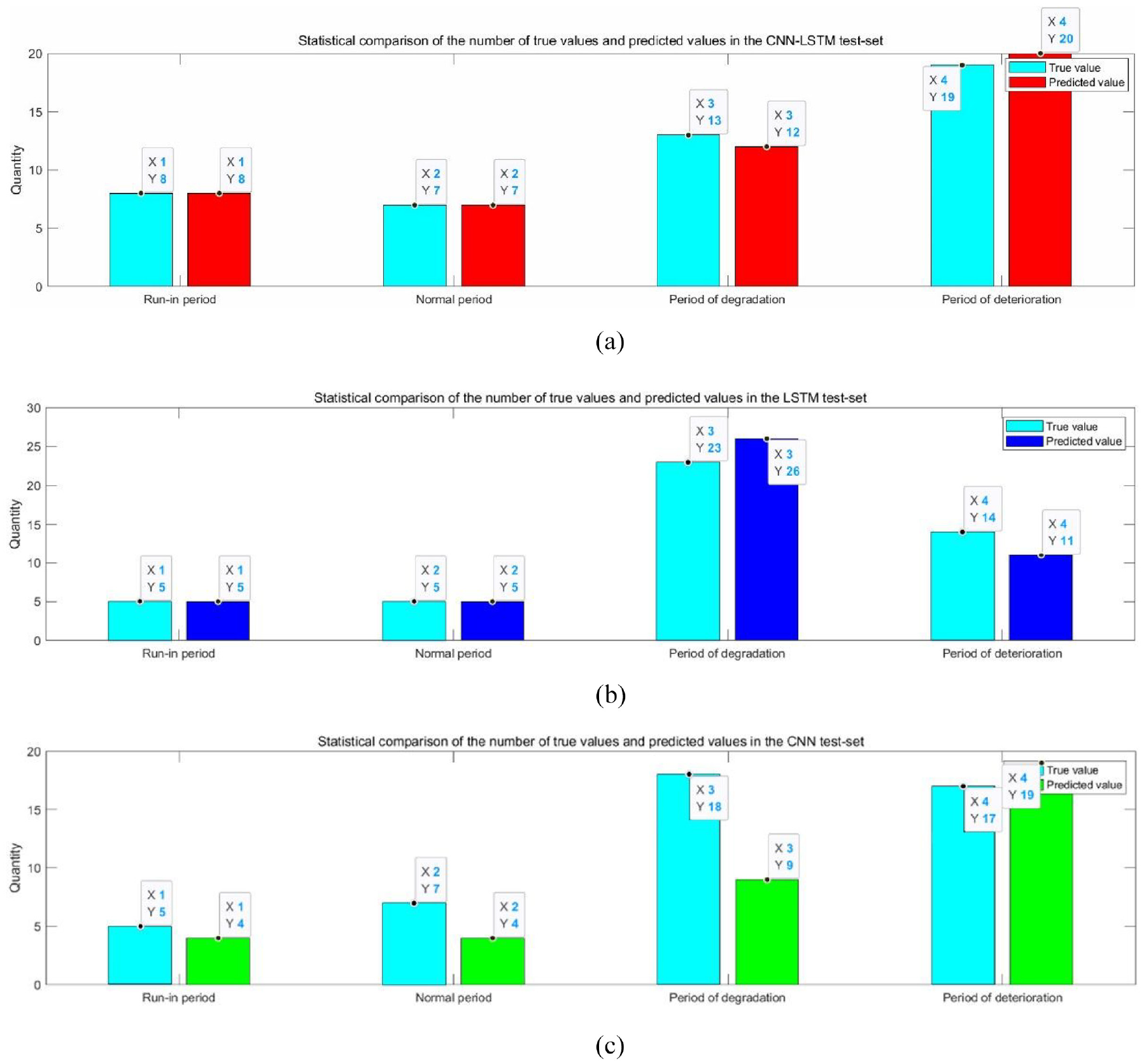
Statistical bar chart of prediction results: (a) statistical results of CNN-LSTM, (b) statistical results of LSTM, and (c) statistical results of CNN.

Figure 12 is a statistical chart displaying both the real values and the predicted values, providing an intuitive representation of the prediction performance of the proposed method. To quantitatively assess the overall performance of the aforementioned method, more detailed error indicators are presented, including Root Mean Square Error (RMSE), Mean Absolute Error (MAE), Mean Square Error (MSE), and Mean Absolute Percentage Error (MAPE), to evaluate its predictive accuracy.¹⁸

1) RMSE is a metric used to quantify the disparity between the predicted and actual values. A smaller RMSE indicates a more accurate alignment between the predicted and actual values. The formula for calculating RMSE is as follows in equation (16):

RMSE = \sqrt{\frac{1}{n} \sum_{i = 1}^{n} {(y_{i} - {\hat{y}}_{i})}^{2}}

(16)

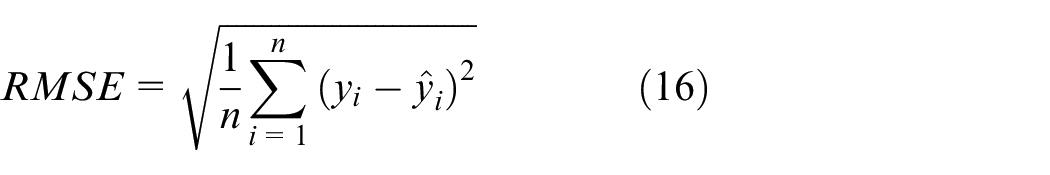
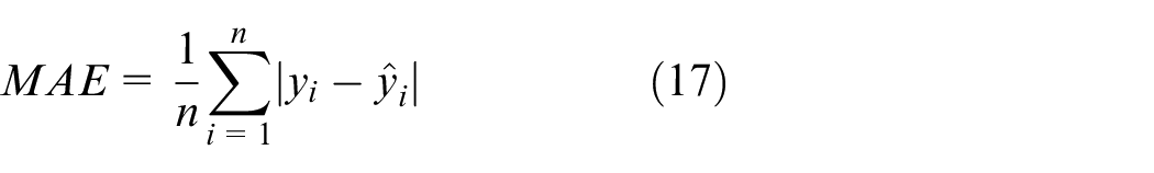
Where n represents the number of samples, y_i represents the true value, and $\hat{y_{t}}$ represents the corresponding predicted value.

2) MAE is a measure of the absolute difference between the predicted value and the true value.²⁰ A smaller MAE indicates a smaller deviation between the predicted and true values. The calculation expression is as follows in equation (17):

MAE = \frac{1}{n} \sum_{i = 1}^{n} | y_{i} - {\hat{y}}_{i} |

(17)

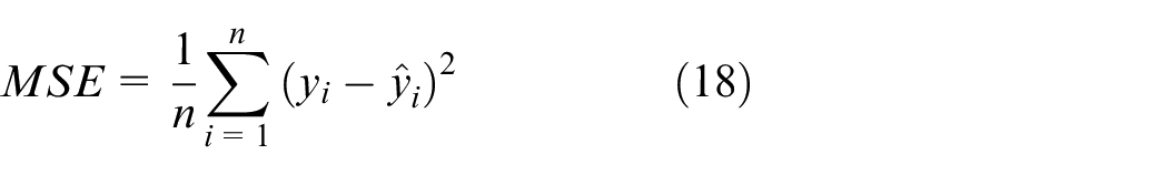
3) MSE is the average of the squared differences between the predicted and true values. It calculates the squared difference between the predicted and true values, sums up these squared differences, and then computes the average. The calculation expression is as follows in equation (18):

MSE = \frac{1}{n} \sum_{i = 1}^{n} {(y_{i} - {\hat{y}}_{i})}^{2}

(18)

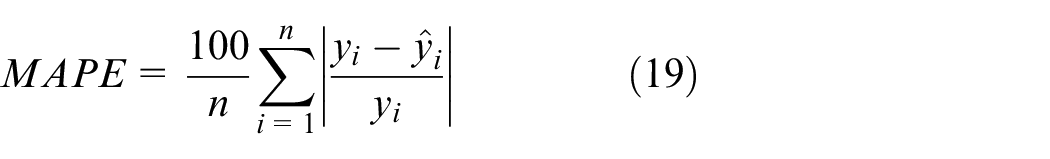
4) MAPE is an average of absolute values that quantifies the percentage difference between predicted and true values. It computes the percentage difference between the predicted value and the true value, takes the absolute value, sums it up, and then calculates the average. The calculation expression is as follows in equation (19):

MAPE = \frac{100}{n} \sum_{i = 1}^{n} | \frac{y_{i} - {\hat{y}}_{i}}{y_{i}} |

(19)

The results for each metric in the test set are presented in Figure 13 below:

Figure 13.

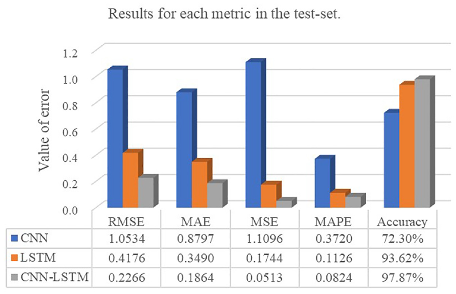
Results for each metric in the test set.

Conclusions and prospects

In this paper, a state estimation method for ball screws is proposed, based on a CNN and LSTM neural network. The life cycle of the ball screw is divided into four stages through the extraction of frequency domain features and the analysis of time series trends in ball screw vibration signals, combined with time domain characteristics. The objective of evaluating the performance and estimating the state of the ball screw is achieved. After experimental verification and result analysis, the following conclusions can be drawn:

1) The CNN and LSTM-based method for estimating the state of the ball screw effectively captures essential features of ball screw vibration signals, encompassing frequency domain amplitudes and temporal trends, thus providing an accurate assessment of the ball screw’s performance state.

2) The proposed method leverages deep learning and demonstrates strong performance in handling complex ball screw performance data. By utilizing feature extraction with a convolutional neural network and time sequence modeling with long short-term memory networks, it effectively captures the performance evolution patterns of the ball screw.

3) The experiments validate that the CNN and LSTM-based state estimation methods exhibit excellent performance concerning prediction accuracy, stability, and robustness. It demonstrates high predictive accuracy and generalization capability, and has important practical significance for estimating the state of the ball screw.

Although the CNN-LSTM-based method for ball screw state estimation has shown promising results, there are several areas warrant further investigation and development.

Firstly, the quality of the data is paramount for ensuring the accuracy of predictive models. Vibration signals may be susceptible to noise interference and uncertainties, potentially leading to inaccuracies in model predictions. Hence, addressing how to effectively preprocess the data and mitigate noise becomes a critical research question. Additionally, obtaining more precise vibration data for ball screws under various operating conditions and loads, and integrating diverse influencing factors such as operating temperature and lubrication status into the state estimation model, represents a crucial avenue for enhancing prediction accuracy and serves as a focal point for future research.

Secondly, the interpretability of the model is a key consideration. While deep learning models exhibit exceptional predictive performance, their internal workings remain intricate and challenging to interpret. Researchers should strive to elucidate how the model captures essential features of ball screw performance, ultimately providing more areas warrant.

Lastly, exploring the application of the CNN-LSTM-based ball screw state estimation method in other industrial equipment and systems holds significant promise. Analogous approaches could be employed for devices featuring vibration signals, such as bearings, fans, engines, etc. This expansion of the method’s application realm would further contribute to its utility and offer support for practical engineering applications in equipment maintenance and health management.

Footnotes

Declaration of conflicting interests

The author(s) declared no potential conflicts of interest with respect to the research, authorship, and/or publication of this article.

Funding

The author(s) disclosed receipt of the following financial support for the research, authorship, and/or publication of this article: This work was supported by the Major basic research projects of equipment (514010507-205).

ORCID iDs

Lei Jianxin

Gao Zhilong

References

Wen

Gao

. Remaining useful life prediction of the ball screw system based on weighted Mahalanobis distance and an exponential model. J Vibroengineering 2018; 20(4): 1691–1707.

Zhang

Gao

Dong

, et al. Wear calculation-based degradation analysis and modeling for remaining useful life prediction of ball screw. Math Probl Eng 2018; 2018: 1–18.

Man

Zheng

Liu

, et al. Bearing remaining useful life prediction based on AdCNN and CWGAN under few samples. Shock Vib 2022; 2022: 1–17.

Song

Shi

Chen

, et al. Remaining useful life prediction of turbofan engine using hybrid model based on autoencoder and bidirectional long short-term memory. J Shanghai Jiaotong Univ (Sci) 2018; 23(S1): 85–94.

Jia

, et al. RUL prediction based on GAM–CNN for rotating machinery. J Braz Soc Mech Sci Eng 2023; 45(142): 1–22.

Peng

Zhang

, et al. Multi-sensor vibration signal based three-stage fault prediction for rotating mechanical equipment. Entropy 2022; 24(2): 164–164.

Zhang

Jiang

Song

, et al. SOC prediction for lithium battery based on the fusion model of attention mechanism and CNN-LSTM. J Power Suppl 2022; 1: 1–15.

Xie

, et al. A hybrid prognostics deep learning model for remaining useful life prediction. Electronics 2020; 10(1): 39–39.

Zhu

Ning

Lei

, et al. Remaining useful life prediction for turbofan engines by genetic algorithm-based selective ensembling and temporal convolutional network. SPE Comput Appl 2020; 12: 3534–3540.

10.

Wang

Zhao

, et al. Adaptive staged RUL prediction of rolling bearing. Measurement 2023; 222(113478): 1–15.

11.

Kundu

Miller

Gore

, et al. Detection of inception of preload loss and remaining life prediction for ball screw considering change in dynamics due to worktable position. Mech Syst Signal Process 2023; 189(110075): 1–18

12.

Jia

Feng

, et al. Prognosability study of ball screw degradation using systematic methodology. Mech Syst Signal Process 2018; 109: 45–57.

13.

Gao

Zhang

Chen

. Monitoring mechanical behaviors of CLT connections under reciprocating loading based on PZT-enabled active sensing and machine learning algorithms. Smart Mater Struct 2023; 32: 024001.

14.

Deng

Shichang

Shiyao

, et al. Prognostic study of ball screws by ensemble data-driven particle filters. J Manuf Syst 2020; 56: 359–372.

15.

Yang

Jiang

Sun

, et al. Remaining Useful Life Prediction of Ball Screw Using Precision Indicator. IEEE Trans Instrum Meas 2021; 70(3519509): 1–9.

16.

Wang

Dong

, et al. A RUL prediction of bearing using fusion network through feature cross weighting. Meas Sci Technol 2023; 34(10): 105908.

17.

Sun

Wang

Gao

, et al. Non-Hertzian elastohydrodynamic contact stress calculation of high-speed ball screws. Appl Sci 2021; 11(24): 12081.

18.

Zhu

Huang

, et al. Bearing remaining useful life prediction of fatigue degradation process based on dynamic feature construction. Int J Fatigue 2022; 164(107169): 1–8.

19.

Lin

Fan

, et al. Structure design and characteristics analysis of a cylindrical giant magnetostrictive actuator for ball screw preload. J Central South Univ 2018; 25(7): 1799–1812.

20.

Wang

Jiang

Yang

, et al. RUL prediction of rolling bearings based on a DCAE and CNN. Appl Sci 2021; 11(23): 11516.

21.

Zhang

Yan

Zhang

, et al. Intelligent monitoring of concrete-rock interface debonding via ultrasonic measurement integrated with convolutional neural network. Constr Build Mater 2023; 400(131865): 1–14.

22.

Chen

Yang

. Illegal network identification optimization based on convolutional neural network. In: Proceedings of the 2018 international conference on network, communication, computer engineering (NCCE 2018). Atlantis Press, 2018.

23.

Yan

Liao

Zhang

, et al. Intelligent monitoring and assessment on early-age hydration and setting of cement mortar through an EMI-integrated neural network. Measurement 2022; 203(111984): 1–16.

24.

Zhang

Liu

. LSTM-Based multi-task method for remaining useful life prediction under corrupted sensor data. Machines 2023; 11(3): 341–341.

25.

Mao

Chen

, et al. A LSTM-STW and GS-LM Fusion method for lithium-Ion Battery RUL prediction based on EEMD. Energies 2020; 13(9): 2380.

26.

Ding

Yin

, et al. A novel method for journal bearing degradation evaluation and remaining useful life prediction under different working conditions. Measurement 2021; 177(109273): 1–17.

27.

Chen

Liu

, et al. A RUL prediction method of small sample equipment based on DCNN-BiLSTM and domain adaptation. Mathematics 2022; 10(7): 1022–1022.

28.

Zhang

Shao

, et al. Rolling Bearing Health Indicator extraction and RUL prediction based on multi-scale convolutional autoencoder. Appl Sci 2022; 12(11): 5747–5747.

29.

Han

, et al. A method for predicting the remaining life of equipment based on WTTE-CNN-LSTM. J Adv Mech Des Syst Manuf 2022; 16(1): JAMDSM0001.

30.

Tian

Wang

. An ensemble learning and RUL prediction method based on bearings degradation indicator construction. Appl Sci 2020; 10(1): 346.

31.

Shan

, et al. A multi-sensor data fusion method for ball screw fault diagnosis based on convolutional neural network with selected channels. IEEE Sens J 2020; 20: 7896–7905.

32.

Xie

Liu

Huang

, et al. Ball screw fault diagnosis based on wavelet convolution transfer learning. Sensors 2022; 22(16): 6270–6270.

33.

Gong

Zhou

, et al. Study on fatigue elastic life of ball screw pair under ultimate load condition. J Instrum Meters 2021; 42(06): 37–47.

34.

Song

Zhai

, et al. Research on remaining useful life prediction method based on CNN and LSTM. In: Abstracts of the 31st Chinese process control conference (CPCC 2020), 2020, p.267.

35.

Liao

Yan

Zhong

, et al. Integrating PZT-enabled active sensing with deep learning techniques for automatic monitoring and assessment of early-age concrete strength. Measurement 2023; 211(112657): 1–16.

A state estimation method based on CNN-LSTM for ball screw

Abstract

Keywords

Introduction

Theoretical background

Degradation process of ball screw

Convolutional neural networks (CNN)

Long short-term memory network (LSTM)

Methods

Vibration signal preprocessing of ball screw

Construction of the CNN-LSTM network

Full life cycle testing and data analysis

Full life cycle testing design of ball screw

Data analysis

Time-frequency analysis

Trend change analysis

State estimation

Division of life cycle stages (label establishment)

Network training process

Analysis of prediction results

Conclusions and prospects

Footnotes

Declaration of conflicting interests

Funding

ORCID iDs

References