Underactuated unmanned surface vehicles formation of obstacle avoidance and assembly: A disturbed fluid-based solution

Abstract

Unmanned surface vehicles (USVs) are highly manoeuvrable and autonomous, and hold significant potential for both military and civilian applications, particularly in formation operations. However, because of their underactuated nature, USVs struggle to navigate in complex maritime conditions during formation. At present, most of the technology is devoted to Unmanned Areial Vehicles and ground robots; these methods cannot be well applied to underactuated USVs. Moreover, the rationality of local path planning decision-making for underactuated USVs formation is still lacking. This study proposes an interfered fluid dynamic system (IFDS)-based local path planning method, called USV-IFDS, specifically designed for the formation of underactuated USVs. This method incorporates the IFDS obstacle avoidance approach, while adapting it through modifications and the inclusion of the kinematic constraints of USVs, thereby enhancing its applicability to the maritime environment. By decomposing the flow field velocity vector and implementing a formation control strategy, we effectively address the challenges in forming underactuated USVs and enhance the efficiency of USV formation local path planning. The proposed formation technique is predicated on the highly robust virtual structure method. Simulations of formation local path planning indicate that our method produces smooth paths, therefore validating its practical applicability to underactuated USV formations.

Introduction

In recent years, the advancement of unmanned and intelligent operations has spurred the rapid development of unmanned surface vehicles (USVs). As a crucial element of unmanned maritime systems, USVs stand out because of their speed, intelligence, size, light weight, high manoeuvrability and agility, cost efficiency and elimination of potential human casualties, compared to traditional surface vehicles. ¹ USVs play a vital role in military activities such as intelligence gathering, reconnaissance, precision attacks and special operations, and therefore, have attracted significant research attention. ² Their diversified functions, higher manoeuvrability and cost efficiency enable them to perform an extensive array of military and civilian tasks, including hydrographic exploration, weather forecasting, maritime search and rescue, and policing and patrol. This versatility suggests a broad scope for their application in the effective utilisation, development and conservation of marine resources. ³

However, the capability of individual USVs to perform diverse maritime operations is inherently limited. As a result, the formation of USVs to enhance their operational efficiency and range has emerged as a mainstream research direction. When compared to individual USVs, the formations of these vehicles offer several advantages^4–6:

• (1) Enhanced operational efficiency: The coordinated control of a group of USVs, optimised decision making and task allocation based on mission requirements, and interactive information communication among multiple USVs enable tasks to be distributed and coordinated effectively. This approach markedly improves the efficiency of task resolution and execution.

• (2) Increased reliability of mission execution: Interactive information communication within a USV formation mitigates the limitations of individual USVs in achieving autonomous, comprehensive perception. This enhancement improves the range and precision of perception and detection, thereby increasing the efficiency of the formation in acquiring and processing target information.

• (3) Improved operational fault tolerance: In the case of individual USVs, a failure of critical equipment can significantly reduce the efficiency or even lead to mission failure. However, with USV formations, the coordinated control and interactive information communication among the multiple USVs enable optimised decision making, timely response and flexible adjustment of the operational plan, providing a better safeguard for successful operation execution.

Therefore, USV formations exhibit superior perception, task execution and fault-tolerance capabilities compared to individual USVs, marking a compelling direction for future technological development.

Underactuated USV formation local path planning is a critical aspect of formation operations and intelligent control, encompassing two main challenges: formation flocking (FF) and obstacle avoidance (OA). Given that USVs lack lateral propulsion, their underactuated nature results in less agility on water surfaces and makes their movement trajectories challenging to track. ⁷ Therefore, a path-planning strategy that enables smooth navigation with high computational efficiency is needed. The virtual structure method, which is simple and highly robust, is employed to maintain a moving flock of USVs in an organised pattern. This method considers the formation shape as a rigid structure, providing clear feedback on the formation shape and enabling better determination and maintenance of the formation behaviour. However, this approach struggles to adapt flexibly and autonomously to complex sea conditions. Moreover, the underactuated nature of USVs (lack of lateral propulsion) limits the flexibility of a USV formation in responding to obstacles for collision avoidance.

State of the art approaches

To address these limitations, we have conducted extensive research and identified the following mainstream solutions: (Table 1)

• (1) geometry-based methods, such as the velocity obstacle method^8–11;

• (2) model predictive control (MPC) methods, for instance, the distributed MPC and neural-dynamic-based nonlinear MPC methods^12,13;

• (3) stochastic planning methods such as the rapidly exploring random tree algorithm and its modified versions^14,15;

• (4) the artificial potential field (APF) method^16–18;

• (5) intelligent optimisation algorithms, for instance, neural networks and reinforcement learning. ¹⁹

Table 1.

Current mainstream solutions.

Solutions	Instance	Disadvantage
Geometry-based methods	Velocity obstacle method	Underactuated USV cannot respond well
Model predictive control (MPC) methods	Distributed MPC method	Lack of rapid response and inefficient computation
Stochastic planning methods	Rapidly exploring random tree algorithm	Calculation efficiency is low in complex environments
The artificial potential field (APF) method	The artificial potential field	More local minimum problems
Intelligent optimisation algorithm	Neural networks and reinforcement learning	Sample inefficiency and lack of flexibility and generalisability

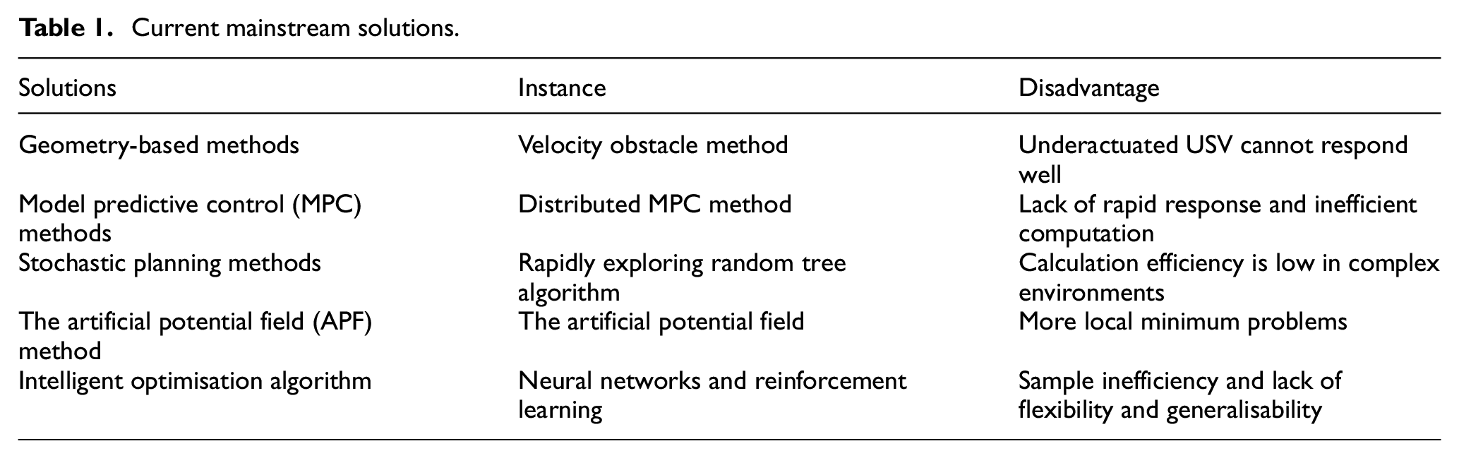
The first three methods generate formation strategies that accommodate the internal structure of a formation and its relationship with obstacle avoidance. However, these strategies are not suitable for USVs because of their underactuated nature and lack of agile response. Moreover, these methods involve computational loads that increase exponentially with the expansion of the operational task and range, leading to inefficient computation for obstacle-free paths and potential loss of tracking targets. The fifth method, reinforcement learning, has the fundamental defect of ‘sample inefficiency’ in obstacle avoidance and lacks flexibility and generalizability; therefore, it does not have good practicability in the obstacle avoidance of underactuated USVs.

A disturbed fluid-based solution

To address these limitations, we have proposed real-time path planning and OA methods inspired by the behaviour of fluids under complex conditions. The most notable among these is the interfered fluid dynamic system (IFDS) method proposed by Wang et al.^20–25 The IFDS method outperforms other fluid behaviour-inspired methods by generating smooth motion paths while maintaining low computational load and high controllability. It offers global optimisation, smooth motion paths and parallel computations, outperforming the APF method by overcoming its local minimum problem. These advantages of the IFDS method over the APF method have also been discussed in previous studies.^20–23 However, traditional IFDS methods do not account for the kinematic characteristics of USVs or the constraints on USV formation. Additionally, they are limited in OA under two-dimensional (2D) conditions and cannot generate a 2D local path planning strategy for the formation of underactuated USVs. To address these issues, this study proposes a USV-specific IFDS local path planning method, called USV-IFDS. This method incorporates the kinematic constraints of USVs, overcomes the limitations of traditional IFDS methods in 2D environments, and ultimately establishes an IFDS strategy suitable for USV formation local path planning.

Model of the problem

Model of obstacles

USV sensor detection of obstacles tends to be excessively precise for path-planning applications. To enhance the efficiency of local path planning, obstacles are abstracted into regular convex shapes. For instance, islands, reefs and shores are represented as triangles, rectangles, hexagons, ellipses, circles or combinations thereof. Moving boats and ships are approximated as circles and ellipses. Hence, obstacles can be expressed using the following equation ²⁶ :

$$\mathrm{\Gamma }\left(\xi \right)=(\frac{{\mathrm{x}}_{\mathrm{t}}-{\mathrm{x}}_0}{\mathrm{a}}{)}^{2c}+(\frac{y_t-y_0}{b}{)}^{2d}$$

(1)

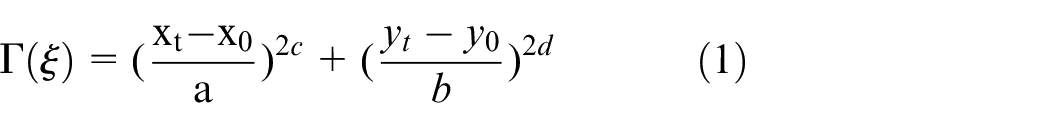
where ξ = (x_t, y_t) represents the USV position at a given moment t and ξ₀ = (x₀, y₀) denotes the centre of the obstacle. The terms a and b are the axial lengths of the obstacle; c and d are the obstacle shape parameters. For an obstacle with sharp boundaries, reasonably chosen axial lengths and shape parameters can moderate the sharpness of the obstacle boundaries to an acceptable extent. This adjustment aligns with USV manoeuvrability constraints and substantially enhances the feasibility of the obstacle avoidance path.

Kinematic model (constraints) of underactuated USVs

The first and most important step to develop the USVs mathematical model is to represent the movement on a 2D plane. ²⁷ Because the focus of this study was path planning and the USV is underdriven and does not have transverse thrust, only its pitch and roll motion are considered. Meanwhile, owing to the minimal planning period and short motion distance of adjacent prediction points, it can be regarded as linear continuous motion. The model is as follows:

$$\{\begin{array}{c}{x}_{t+1}=x_t+V_{\mathrm{t}}\mathrm{\Delta }t\cos ({\theta }_t)\hfill \\ \multicolumn{1}{c}{y_{t+1}=y_t+V_t\mathrm{\Delta }t\sin ({\theta }_t)}\\ \multicolumn{1}{c}{{\theta }_{t+1}={\theta }_t+{\omega }_t\mathrm{\Delta }t}\end{array}$$

(2)

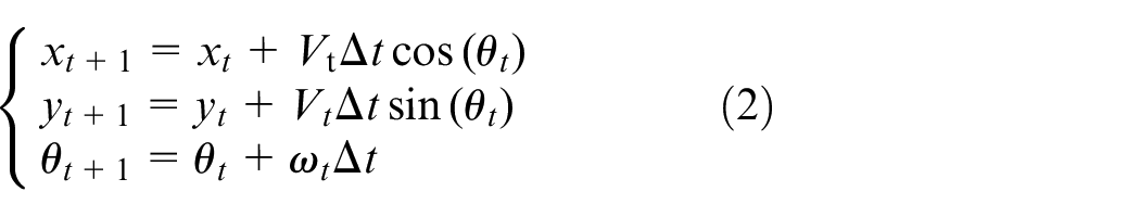
where x_t, y_t, θ_t, V_t and ω_t denote the x-coordinate, y-coordinate, course angle, velocity amplitude and steering angular velocity of the USV in the geodetic coordinate system at a given moment t, respectively.

Considering the limitations in USVs power and direction-changing ability as well as the constraints on their manoeuvrability, the USV velocity vector, ${\stackrel{\rightharpoonup }{V}}_{\lim }$ , can be expressed as

$${\stackrel{\rightharpoonup }{V}}_{\lim }=\{(V,\omega )|v\in [V_{\min },V_{\max }],\omega \in [{\omega }_{\min },{\omega }_{\max }]$$

(3)

The actual velocity at the next moment, V_t+1, can be expressed as

$${\stackrel{\rightharpoonup }{V}}_{\mathrm{t}+1}=\{(V_{t+1},{\omega }_{t+1})|V_{t+1}\in [V_t-a_{v-}\mathrm{\Delta }t,V_t+a_{v+}\mathrm{\Delta }t],{\omega }_{t+1}\in [{\omega }_t-a_{\omega }\mathrm{\Delta }t,{\omega }_t+a_{\omega }\mathrm{\Delta }t]$$

(4)

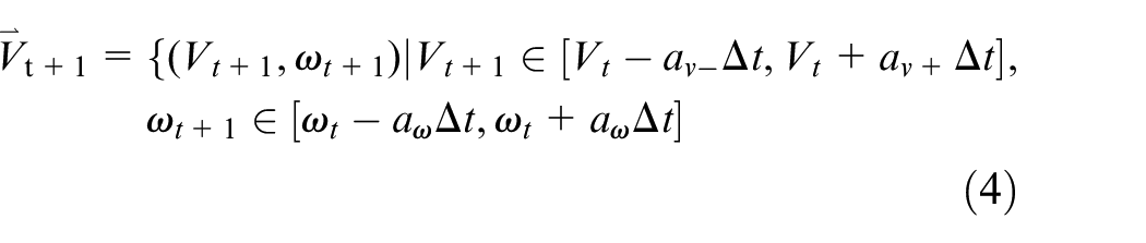
where (V_min, V_max) represents the velocity range; (ω_min, ω_max) represents the steering angular velocity range; and α_v-, α_v+ and α_ω refer to the deceleration, acceleration and steering performances of the velocity, respectively.

USV-IFDS local path planning method

Description of the IFDS method

The traditional IFDS method contemplates three-dimensional OA. However, given that ships can only move on the water surface and their manoeuvrability is limited, only the 2D aspect of the IFDS method is discussed here. Prior to path planning using the IFDS method, all obstacles are modelled using equation (1), with the destination set as ξ_d = (x_d, y_d) and the number of obstacles denoted as K.

When the USV is positioned on an obstacle-free water surface, the initial flow field is established considering the path from the USV current position at a given moment t to the destination as a straight line with a velocity amplitude of V. Hence, the initial flow field along the two axes of the geodetic coordinate system, u, can be expressed as

$$u_t={\left[\begin{array}{c}\frac{V(x_d-x_t)}{d}\frac{V(y_d-y_t)}{d}\hfill \end{array}\right]}^T$$

(5)

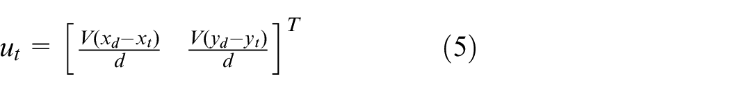
where $d=\sqrt{{(x_t-x_d)}^2+{(y_t-y_d)}^2}$ is the distance from the USV position at moment t to the destination.

When the USV is positioned on a water surface with K obstacles, the total disturbance of the obstacles to the initial flow field μ_t can be expressed in matrix form ( $\overline{M}$ ):

$$\overline{M}=\sum _{k=1}^K{W}_k{M}_k$$

(6)

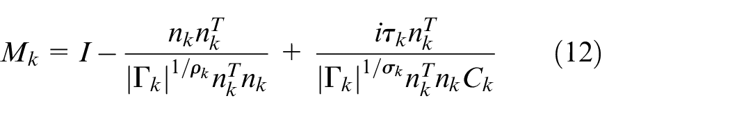
where W_k is the weight of the kth obstacle, which increases as the distance between the obstacle and USV decreases, and M_k is the disturbance matrix of the kth obstacle. W_k and M_k can be expressed as

$$W_k=\{\begin{array}{c}1\hfill \\ \multicolumn{1}{c}{{\Pi }_{i=1,i\ne k}^K\frac{({\mathrm{\Gamma }}_i-1)}{({\mathrm{\Gamma }}_i-1)+({\mathrm{\Gamma }}_k-1)}}\end{array}\begin{array}{c}K=1\hfill \\ \multicolumn{1}{c}{K\ne 1}\end{array}$$

(7)

$$M_k=I-\frac{n_k{n}_k^T}{{\left|{\mathrm{\Gamma }}_k\right|}^{1/{\rho }_k}{n}_k^T{n}_k}$$

(8)

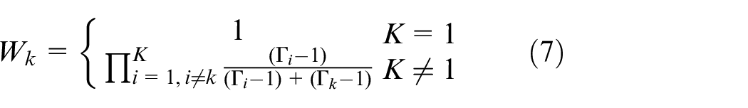
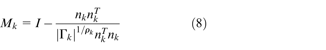
where I is the attraction matrix (a second-order identity matrix illustrating the effects of the destination on the USV); $-\frac{n_k{n}_k^T}{{\left|{\mathrm{\Gamma }}_k\right|}^{1/{\rho }_k}{n}_k^T{n}_k}$ is the repulsion matrix (representing the effects of the obstacle on the initial flow field); ρ_k is the repulsion coefficient (adjusting the OA response of the USV to the obstacle, where a larger ρ_k value indicates a stronger OA response to the obstacle); and $n^k={\left[\begin{array}{c}\frac{\partial {\mathrm{\Gamma }}_k}{\partial x}\frac{\partial {\mathrm{\Gamma }}_k}{\partial y}\hfill \end{array}\right]}^{\mathrm{T}}$ is the normal vector of the obstacle surface.

Subsequently, moving obstacles such as ships and platforms are taken into account to facilitate dynamic OA. Consequently, the original flow velocity u_t is adjusted. The resulting total interfered flow velocity can be expressed as

$$\overline{u_t}=\overline{M}(u_t-v_{\mathrm{\Gamma }})+v_{\mathrm{\Gamma }}$$

(9)

where v_Г is the total velocity vector of the obstacles and can be expressed as

$$v_{\mathrm{\Gamma }}=\sum _{k=1}^K{W}_k{e}^{\frac{1-{\mathrm{\Gamma }}_k}{{\lambda }_k}}{v}_{{\mathrm{\Gamma }}_k}$$

(10)

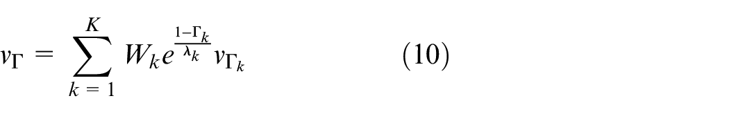
where λ_k is the constant of the kth obstacle and v_Гk is the velocity vector of the kth obstacle. Accordingly, ${\overline{u}}_{\mathrm{t}}={\left[\begin{array}{c}\overline{u_{x_t}}\overline{u_{y_t}}\hfill \end{array}\right]}^{\mathrm{T}}$ , and the USV position at the next moment is updated as ${\xi }_{\mathrm{t}+1}=(x_{t+1},y_{t+1})=(x_t+\overline{u_{x_{\mathrm{t}}}}\mathrm{\Delta }t,y_t+\overline{u_{y_t}}\mathrm{\Delta }t)$ , where Δt represents the sampling time. Finally, a motion path can be obtained by integrating the USV position with respect to the sampling time.

The aforementioned method exhibits the following characteristics:

• Theorem 1: When the USV is at a considerable distance from any obstacle, its motion path follows a straight line in the original direction.

• Theorem 2: Obstacles cannot be penetrated.

Proof: (1) When the USV is far from any obstacle, because ${\mathrm{\Gamma }}_k=\infty$ , ${\overline{u}}_t=u_t$ .

(2) If the USV is positioned at the surface of an obstacle, ensuring that the normal velocity remains at zero will prevent the obstacle from being penetrated. Hence, it is only necessary to demonstrate that $n_k^T\overline{u_t}=0$ . Because Г _k  = 1 when the USV is located at the obstacle’s surface and $n_k^T{M}_k=n_k^T-\frac{n_k^T{n}_k{n}_k^T}{n_k^T{n}_k}=n_k^T-n_k^T=0$ , the condition that an obstacle cannot be penetrated is satisfied.

Description of the USV-IFDS

The previous derivation illustrates that the conventional IFDS method for 2D path planning does not account for the kinematic constraints of USVs. Therefore, this study introduces the USV-IFDS method, which takes the kinematic constraints of USVs into account using a kinematic model, ensuring the feasibility of motion paths.

Let us denote the current course angle of the USV at moment h as θ_h; the interfered flow velocity obtained using equation (9), ${\overline{u}}_{\mathrm{h}}={\left[\begin{array}{c}\overline{u_{x_h}}\overline{u_{y_h}}\hfill \end{array}\right]}^{\mathrm{T}}$ , represents the expected OA velocity at the next moment. From this relation, the expected course angle can be determined: $\tan {\theta }_{\mathrm{h}+1}=\frac{\overline{u_{y_h}}}{\overline{u_{x_h}}}$ . Hence, the expected steering angular velocity becomes ${\omega }_{\mathrm{h}}=\frac{{\theta }_{h+1}-{\theta }_h}{\mathrm{\Delta }t}$ .

Considering the constraint of angular velocity, the actual output course angle, θ_true, can be derived:

$${\theta }_{\mathrm{t}\mathrm{rue}}=\{\begin{array}{cc}{\theta }_{h+1}\hfill & {\omega }_{min}\le {\omega }_h\le {\omega }_{max}\hfill \\ \multicolumn{1}{c}{{\theta }_h+\mathrm{\Delta }t{\omega }_{max}}& {\omega }_{max}\le {\omega }_h\hfill \\ \multicolumn{1}{c}{{\theta }_h+\mathrm{\Delta }t{\omega }_{min}}& {\omega }_h\le {\omega }_{min}\hfill \end{array}$$

(11)

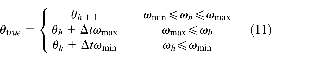
By replacing the expected course angle with the constrained course angle, θ_true, the actual course angle at the following moment can be derived. The output-constrained course angle can be substituted into equation (2) to derive the position of the USV at the next moment.

Method for solving local minima

The USV-IFDS path planning method outlined in the previous section can effectively simulate the path of natural water flow and overcomes the local minimum problem associated with the APF method. However, it is evident that the USV-IFDS method still encounters issues with stagnation points and trap areas. To better resolve these problems, we made modifications to ensure the feasibility of the motion paths.

Stagnation point analysis and improvement solution

Figure 1 illustrates the situation where the USV, goal and obstacle are in a straight line.

Figure 1.

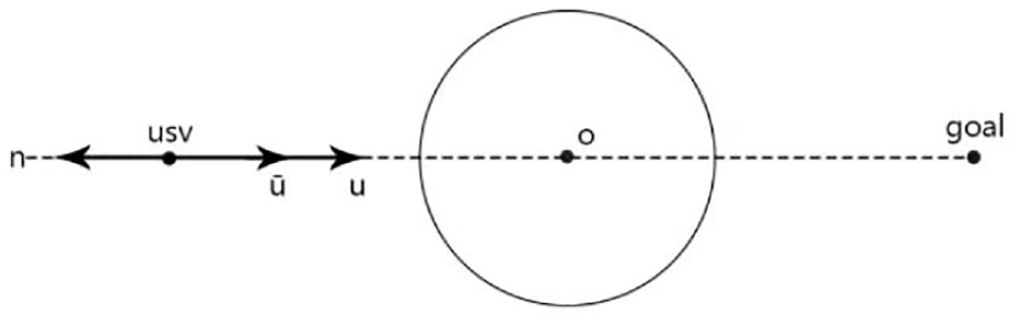
Stagnation point example.

When the USV moves to the centre of an obstacle with the goal directly behind the obstacle, the initial flow field from the goal to the USV (u) and the repulsion flow field from the obstacle to the USV (n) are collinear but in opposite directions. This situation results in a decreasing total flow field velocity $\overline{u}$ , which exactly equals zero when the USV reaches the surface of the obstacle. Consequently, the USV stagnates at that point, creating a stagnation point under 2D conditions.

To overcome this problem, we introduced an escape matrix to improve the stagnation point issue of the USF-IFDS in 2D planes. We first obtain a tangent vector ${\tau }_k={\left[\begin{array}{c}\frac{\partial {\mathrm{\Gamma }}_k}{\partial y}-\frac{\partial {\mathrm{\Gamma }}_k}{\partial x}\hfill \end{array}\right]}^{\mathrm{T}}$ that is perpendicular to the normal vector n_k of the obstacle surface. This tangent vector is incorporated into a matrix added to equation (8):

$$M_k=I-\frac{n_k{n}_k^T}{{\left|{\mathrm{\Gamma }}_k\right|}^{1/{\rho }_k}{n}_k^T{n}_k}+\frac{i{\tau }_k{n}_k^T}{{\left|{\mathrm{\Gamma }}_k\right|}^{1/{\sigma }_k}{n}_k^T{n}_k{C}_k}$$

(12)

Here, the newly added term, $\frac{i{\tau }_k{n}_k^T}{{\left|{\mathrm{\Gamma }}_k\right|}^{1/{\sigma }_k}{n}_k^T{n}_k{C}_k}$ , represents the escape matrix, which operates on similar principles as the repulsion matrix. The tangent vector τ_k is projected onto the initial flow field to adjust the effects of the initial flow field. $i\in [-1,1]$ is used to adjust the escape direction, causing the USV to veer towards the right boundary if it is closer to the right boundary, and towards the left boundary if it is closer to the left boundary. The escape coefficient of the kth obstacle is represented by σ_k, with a larger escape coefficient indicating a faster speed to avoid the stagnation point. We introduce a constant, C_k, to mitigate its effect on OA performance. If C_k is assigned a reasonable value, the magnitude of the escape matrix is considerably smaller than that of the repulsion matrix, which minimises its effect on the original motion path and avoids the creation of sharp curves.

When the USV is heading towards the stagnation point, the tangent vector τ_k helps the USV to deviate slightly in the direction perpendicular to the course, thus escaping from the stagnation point.

The proof that the escape matrix does not affect the course is as follows: When the USV is at the surface of the obstacle, because $n_k^{T}i{\tau }_k=0$ , $n_k^T\overline{u}=0$ ; that is, theorem 1 is satisfied. When the USV is far away from any obstacle, because Г_k increases monotonically as the USV moves away from the obstacle and C_k affects the escape matrix, the norm of the escape matrix is infinitesimal, that is, theorem 2 is satisfied. Hence, the flow field with the addition of the escape matrix still satisfies the requirements for path planning.

Trap area problem and improvement solution

The issue of ‘trap areas’ arises when multiple overlapping obstacles are present in the planning space, enclosed by the common tangent of the two circles and the boundaries of the obstacles as shown in Figure 2; this situation forms an enclosed space or ‘trap’ to the trap situation occurs because of a limitation in the algorithm. When the USV is located at the junction of two obstacles, both Г _k and Г _k+1 equal 1, causing the denominator of equation (7) used for weight calculation to become 0. As a result, navigation planning fails. This issue is particularly likely to occur when the two obstacles are large, parallel-moving ships. To mitigate navigation collision risks and take into account the limited manoeuvrability of underactuated USVs, a virtual goal strategy can be employed to navigate around these trap areas.

Figure 2.

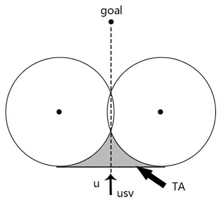
Trap area example.

First, when a trap area is identified, a virtual goal is created on the basis of the following observations:

• (1) The presence of multiple overlapping obstacles;

• (2) The interfered flow velocity $\overrightarrow{u}$ moving towards the trap area;

• (3)  $min\{d(\xi ,{\xi }_1),d(\xi ,{\xi }_2),d(\xi ,{\xi }_3),...d(\xi ,{\xi }_k)\}\le d_{\mathrm{TA}}$ .

Here, d_TA represents a threshold value, which is established considering factors such as the manoeuvrability of the USV, number of overlapping obstacles and area of the trap. D(ξ, ξ_k) measures the distance from the USV to the kth obstacle.

Figure 3 illustrates a scenario where all these conditions are fulfilled. A circular sector is defined with the centre of the USV model serving as the origin, a radius of d_TA and a central angle derived from the course angle of the USV and the maximum turning angle, which falls within the range (θ_t − φ_max, θ_t + φ_max).

Figure 3.

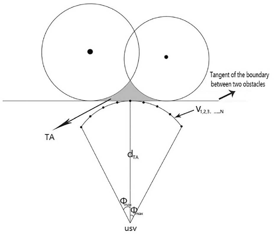
Creation of a virtual goal.

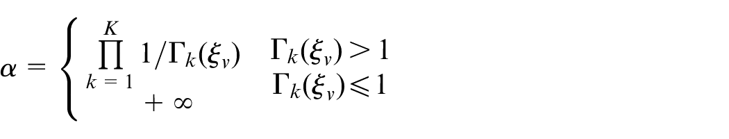
N discrete points, represented as v (virtual goals), are chosen on the arc. These N points form a set of optimal options v_1,2,3…N for the virtual goal. Lastly, the N virtual goals are assessed, with a lower cost function value indicating a superior choice for the virtual goal. The cost function, eval, is given as follows:

$$\mathrm{eval}={\lambda }_1\alpha +{\lambda }_2\beta +{\lambda }_3\vartheta$$

(13)

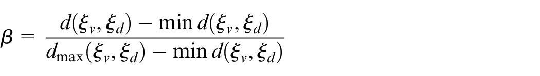
Here, (λ₁, λ₂, λ₃) are the weights, α represents the safety cost for determining whether the USV collides with an obstacle, β represents the distance cost for determining the extra distance of movement and $\vartheta$ represents the escape cost for determining whether the USV has escaped from the trap area.

$$\alpha =\{\begin{array}{c}\underset{k=1}{\overset{K}{\Pi }}1/{\mathrm{\Gamma }}_k({\xi }_v)\hfill \\ \multicolumn{1}{c}{+\infty }\end{array}\begin{array}{c}{\mathrm{\Gamma }}_k({\xi }_v)>1\hfill \\ \multicolumn{1}{c}{{\mathrm{\Gamma }}_k({\xi }_v)\le 1}\end{array}$$

$$\beta =\frac{d({\xi }_v,{\xi }_d)-mind({\xi }_v,{\xi }_d)}{d_{max}({\xi }_v,{\xi }_d)-mind({\xi }_v,{\xi }_d)}$$

$$\vartheta =\{\begin{array}{c}0\hfill \\ \multicolumn{1}{c}{+\infty }\end{array}\begin{array}{c}\mathrm{from}\mathrm{USV}\mathrm{to}v\mathrm{without}\mathrm{passing}\mathrm{throug}\mathrm{the}\mathrm{trap}\mathrm{area}\hfill \\ \multicolumn{1}{c}{\mathrm{Otherwise}}\end{array}$$

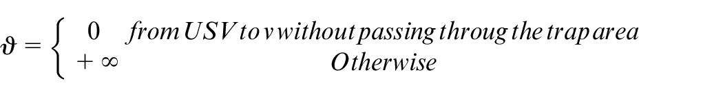
When the virtual goal satisfies the cost function and feasibility requirements, the USV advances to the virtual target point and after driving to the virtual target point, it sails to the target point again, thereby escaping the trap area.

Formation local path planning using the USV-IFDS method

The preceding explanation covers local path planning for a single USV using the USV-IFDS method, which makes the IFDS method more suitable for the specific operating environment of USVs. To further refine this method for formation coordination, we break down the formation problem into two aspects: local path planning for FF and local path planning for formation OA. To simplify the problem and make the method more practical, we consider these two aspects separately. For formation maintenance, given the stability and safety requirements of an underactuated USV formation, we employ a highly robust virtual structure method as our formation strategy. In other words, we treat the entire formation as a rigid body.

Formation flocking strategy

The local path planning for individual USVs during FF considers the constraints of a single USV described in Section ‘A disturbed fluid-based solution’ as well as the requirements for OA and FF. We assume that there are only a small number of obstacles in the path of flocking, as illustrated in Figure 4.

Figure 4.

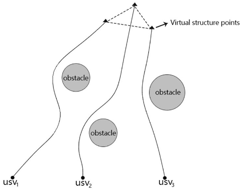
Formation flocking example.

Here, we use the virtual structure points associated with individual USVs as the respective goals of their initial flow fields. Given the rock-avoidance characteristic of water flow, which is fundamental to the IFDS method, each USV can effectively avoid obstacles and reach the assembly point through the shortest possible path. Furthermore, to ensure the task execution by a USV formation is both efficient and feasible, we consider two things. First, we treat the virtual structure points (the goals of the initial flow fields) as dynamic goals during the configuration of the initial flow fields. This approach allows a task to be assigned to a USV formation before the individual USVs reach their designated positions, significantly reducing the time needed for FF and task execution. Second, it is possible that the path of a USV flocking to the assembly point intersects with that of another USV. To ensure safe and simultaneous flocking, we treat each USV as a dynamic obstacle for the others. Furthermore, we decouple the vectors and scalars of each USV initial flow field. As a result, equation (5) is broken down into velocity amplitude V and vector ${\left[\begin{array}{c}\frac{x_d-x_t}{d}\frac{y_d-y_t}{d}\hfill \end{array}\right]}^T$ . The velocity amplitude is then adjusted according to the distance to the virtual structure point, as demonstrated in Figure 5.

Figure 5.

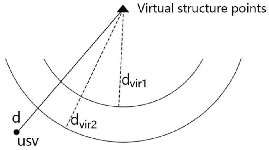
Distance to a virtual structure point.

The relationship between the velocity amplitude and distance is characterised as

$$V=\{\begin{array}{c}\begin{array}{c}{V}_{max}\hfill \\ \multicolumn{1}{c}{V_{\mathrm{vir}}+(V_{max}-V_{\mathrm{vir}})e^{-{\lambda }_{\mathrm{vir}2}(d_{\mathrm{vir}2}-d)}}\\ \multicolumn{1}{c}{V_{\mathrm{vir}}{e}^{-{\lambda }_{\mathrm{vir}1}(d_{\mathrm{vir}1}-d)}}\end{array}\begin{array}{c}d\ge d_{\mathrm{vir}2}\hfill \\ \multicolumn{1}{c}{d_{\mathrm{vir}1}\le d<d_{\mathrm{vir}2}}\\ \multicolumn{1}{c}{d<d_{\mathrm{vir}1}}\end{array}\hfill \end{array}$$

(14)

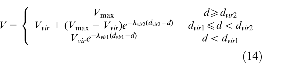
where V_max represents the maximum velocity amplitude and V_vir is the presupposed velocity of the virtual structure point. The variables d_vir1 and d_vir2 are threshold values for the distance to the virtual structure point, and d is the actual distance from the USV to the virtual structure point. λ_vir1 and λ_vir2 are the constants to adjust the velocity magnitudes at the two distance thresholds. According to equation (14), when outside d_vir2, the USV moves closer to the virtual target point at the maximum speed, and when inside d_vir1, the USV slows and moves away from the virtual target point; thus, we can effectively manage the velocity magnitude of each USV so that it aligns with the presupposed velocity. Adjusting d_vir1 and d_vir2 enables us to control the distance from the USV to the virtual structure point, thereby enhancing the reliability of FF. Furthermore, once a USV moves into the interval between d_vir1 and d_vir2, other USVs are no longer considered obstacles. This approach ensures that individual USVs within a formation do not interfere with one another during formation navigation.

When every USV in the formation has moved into the interval between d_vir1 and d_vir2 relative to its corresponding virtual structure point, the formation has successfully completed the flocking phase and can begin the formation navigation phase.

Formation OA strategy

The interfered flow field-based OA strategy designed for a single USV is also utilised for formation OA. A USV retains its agility whether it is navigating individually or within a formation. Furthermore, because of the inherent properties of the flow fields, their streamlines do not intersect even when they share the same response coefficient for the same obstacle. This feature provides a certain degree of safety during formation OA. However, there are still challenges, as illustrated in Figure 6.

Figure 6.

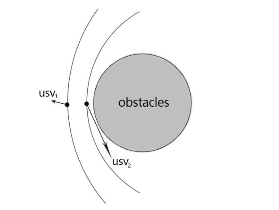
Formation OA example.

When two or more USVs are on the same side of an obstacle, their streamlines do not intersect, but the space between the streamlines may become excessively small. Given that actual USVs are not mass points but objects with a certain volume, this situation could be unsafe for formation navigation. If each USV is considered an obstacle to the others as during FF (as described in Section ‘Formation flocking strategy’), the OA performance of the USVs will be significantly compromised. Therefore, a new solution is needed for this problem.

For a formation consisting of F_tot USVs to avoid the kth obstacle, the disturbance matrix M_k for each USV is computed using equation (12). Then, the formation matrix is added to account for the effects of the other F_tot − 1 USVs on the current USV. The formation matrix of the fth USV in the formation affecting the current USV is expressed as $\frac{{\chi }_f{n}_k^T(1-e^{1-{\mathrm{\Gamma }}_k})}{{\left|{\mathrm{\Gamma }}_k\right|}^{1/{\rho }_{\mathrm{kf}}}\Vert {\chi }_f\Vert \Vert n_k^T\Vert }{F}_f$ . A matrix is added for each additional USV. This formation matrix can make the USV move away from the other USVs corresponding to each matrix through the repulsion vector. The final total disturbance matrix is expressed as

$$\begin{array}{c}\multicolumn{1}{c}{M_k=I-\frac{n_k{n}_k^T}{{\left|{\mathrm{\Gamma }}_k\right|}^{1/{\rho }_k}{n}_k^T{n}_k}+\frac{i{\tau }_k{n}_k^T}{{\left|{\mathrm{\Gamma }}_k\right|}^{1/{\sigma }_k}{n}_k^T{n}_k{C}_k}+\frac{{\chi }_f{n}_k^T(1-e^{1-{\mathrm{\Gamma }}_k})}{{\left|{\mathrm{\Gamma }}_k\right|}^{1/{\rho }_{\mathrm{kf}}}\Vert {\chi }_f\Vert \Vert n_k^T\Vert }{F}_f}\\ \multicolumn{1}{c}{+\frac{{\chi }_{f+1}{n}_k^T(1-e^{1-{\mathrm{\Gamma }}_k})}{{\left|{\mathrm{\Gamma }}_k\right|}^{1/{\rho }_{\mathrm{kf}+1}}\Vert {\chi }_{f+1}\Vert \Vert n_k^T\Vert }{F}_{f+1}.....+\frac{{\chi }_{\mathrm{Ftot}-1}{n}_k^T(1-e^{1-{\mathrm{\Gamma }}_k})}{{\left|{\mathrm{\Gamma }}_k\right|}^{1/{\rho }_{\mathrm{kFtot}-1}}\Vert {\chi }_{\mathrm{Ftot}-1}\Vert \Vert n_k^T\Vert }{F}_{\mathrm{Ftot}-1}}\end{array}$$

(15)

where ${\chi }_f={\left[\begin{array}{c}{x}_f-x_t{y}_f-y_t\hfill \end{array}\right]}^T$ is the repulsion vector of the fth USV to the current USV (where (x_f, y_f) is the predicted position of the fth USV at the next moment); $\Vert •\Vert$ is the 2-norm of the vector; ρ_kf is the modulation coefficient of the formation matrix of the effects of the fth USV on the current USV during OA, with a larger modulation coefficient indicating better performance; and F_f is the response coefficient, which changes with the distance from the fth USV to the current USV and is expressed as

$$F_f=\{\begin{array}{c}\begin{array}{c}\frac{e^{d_w-d_f}}{2}{d}_f\ge d_w\hfill \end{array}\hfill \\ \multicolumn{1}{c}{\begin{array}{c}1-\frac{e^{d_f-d_w}}{2}{d}_f<d_w\hfill \end{array}}\end{array}$$

(16)

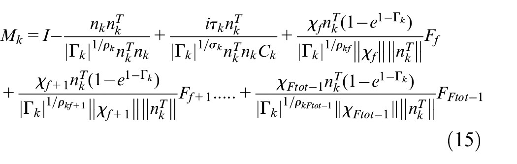
where d_f is the distance from the fth USV to the current USV and d_w is the warning distance for the current USV. Equation (16) decreases monotonically, is continuous, and converges between 0 and 1. Thus, F_f decreases as the distance increases and converges at 0 as the distance increases to a certain value. F _f increases as the distance decreases and converges at 1 when the distance decreases to a certain value.

Similar to the proof of escape, the reasonableness of the formation matrix is demonstrated as follows: When the USV is far from any obstacle, ${\mathrm{\Gamma }}_k=\infty$ and consequently, $1-e^{1-{\mathrm{\Gamma }}_k}$ is approximately equal to 1, the formation matrix is infinitesimal, and theorem 1 is satisfied. When the USV is at the obstacle surface, because ${\mathrm{\Gamma }}_k=1$ , $1-e^{1-{\mathrm{\Gamma }}_k}=0$ , the formation matrix equals 0, and $n_k^T\overline{u}=0$ ; that is, theorem 2 is satisfied.

Simulation

Case study using the USV-IFDS and IFDS methods

Comparison of imposed constraints

Unlike the IFDS method, the USV-IFDS method accounts for kinematic constraints. To demonstrate that the USV-IFDS method is more appropriate under 2D conditions, a path planning case was simulated using both methods separately. The conditions were as follows: starting point of (1, 1) m, goal of (200, 200)  m, USV course angle θ = 45°, velocity V = 7.5 m/s (uniform), centre of obstacle at (100, 90) m, obstacle radius of 25 m and repulsion coefficient ρ_k = 3 (to ensure that the variables have unique values for both the USV-IFDS and IFDS methods). Figure 7 shows the angular velocities produced by the two methods.

Figure 7.

Angular velocities yielded by the USF-IFDS (constraint: maximum angular velocity 0.1 rad/s) and IFDS methods.

As illustrated in Figure 7, the USV-IFDS method more effectively adheres to the kinematic constraints compared to the IFDS method.

Comparison of local minima

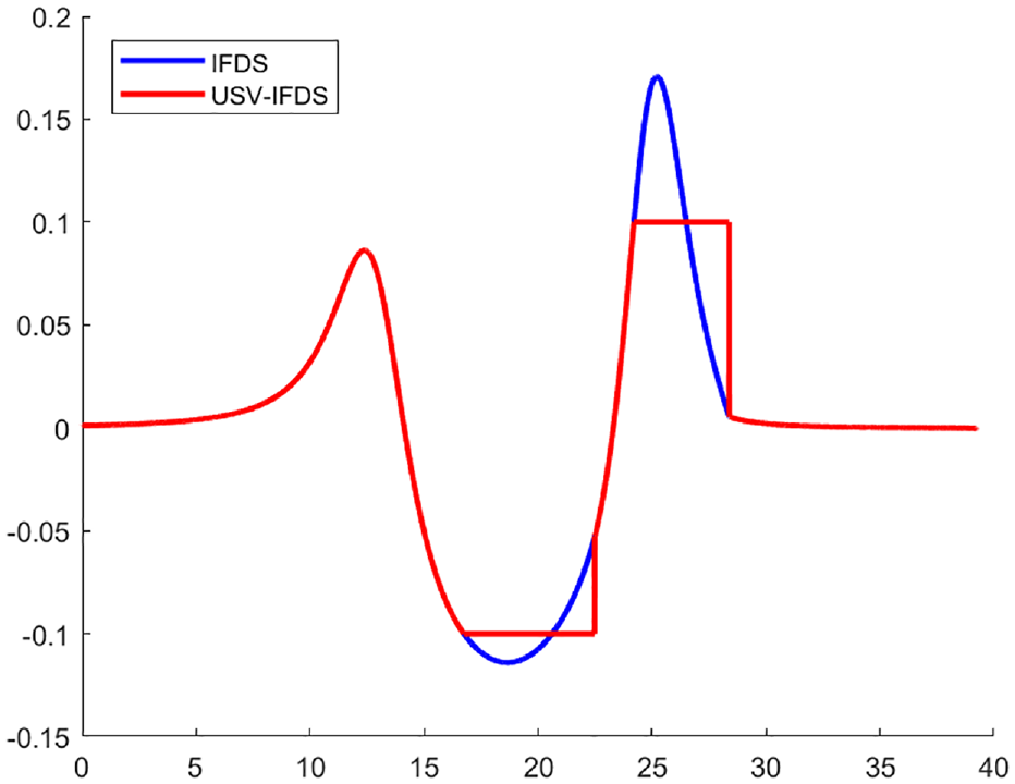
Unlike the traditional IFDS method, the USV-IFDS method effectively resolves the issue of stagnation points. To compare these two methods in this regard, a stagnation point avoidance problem was separately solved using both methods under the following conditions: starting point of (1, 1) m, goal of (100, 100) m, course angle θ = 45°, velocity V = 7.5 m/s (uniform), centre of the obstacle at (50, 50) m, obstacle radius of 15 m and repulsion coefficient ρ_k = 3 for both methods. For the USV-IFDS method, the escape coefficient σ_k was set to 1, and the constant C_k was set to 10. The results are shown in Figure 8.

Figure 8.

Comparison of stagnation point avoidance performance: (a) IFDS method and (b) USV-IFDS method.

The USV-IFDS method demonstrated strong capabilities in navigating away from stagnation points and effectively resolving stagnation point issues. It produced a path that not only complied with OA requirements but was also smooth, thereby validating its exceptional effectiveness in local OA planning for underactuated USVs.

In addition, the USV-IFDS method successfully addressed the trap area issue. This was confirmed with the following test case: start point of (1, 1) m, goal of (100, 100) m, USV angle θ = 45°, velocity V = 7.5 m/s (uniform), centre of obstacle #1 at (50, 60) m, centre of obstacle #2 at (60, 50) m, radii of both obstacles of 15 m, repulsion coefficient ρ_k = 3, escape coefficient σ_k of 1 and constant C_k of 10. The results are presented in Figure 9.

Figure 9.

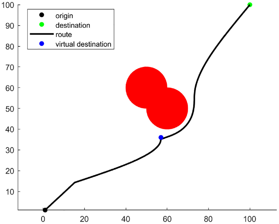
Configuration of virtual goal for escaping from a trap area using the USV-IFDS method. The method succeeded in generating a virtual goal and escaping from the trap area.

Formation local path planning (formation flocking)

The performance of the USV-IFDS method in local path planning for FF was verified by simulating the flocking of three USVs using the following parameter settings: The starting positions for USV #1, #2 and #3 were (10, 10) m, (40, 1) m and (1, 40) m, respectively; the maximum velocity was 23 m/s (approximately 45 knots); the course angle θ was 45°; the repulsion coefficient ρ_k was 3; the escape coefficient σ_k was set at 1; and the constant C_k was set at 10. The centres of the three obstacles were located at (80, 60) m, (30, 50) m and (100, 110) m, with radii of 9, 12 and 11 m, respectively. The initial positions of the virtual structure points for USV #1, #2 and #3 were (150, 120) m, (150, 150) m and (120, 150) m, respectively. The uniform velocity of the virtual structure formation was 7.5 m/s (approximately 15 knots), with a course angle θ of 45°. The distance thresholds were d_vir1 = 10 m and d_vir2 = 11 m. The velocity magnitude adjustment constants at the distance thresholds were λ_vir1 = 0.5 and λ_vir2 = 8. Figure 10 illustrates the movement trajectories of the flocking USVs.

Figure 10.

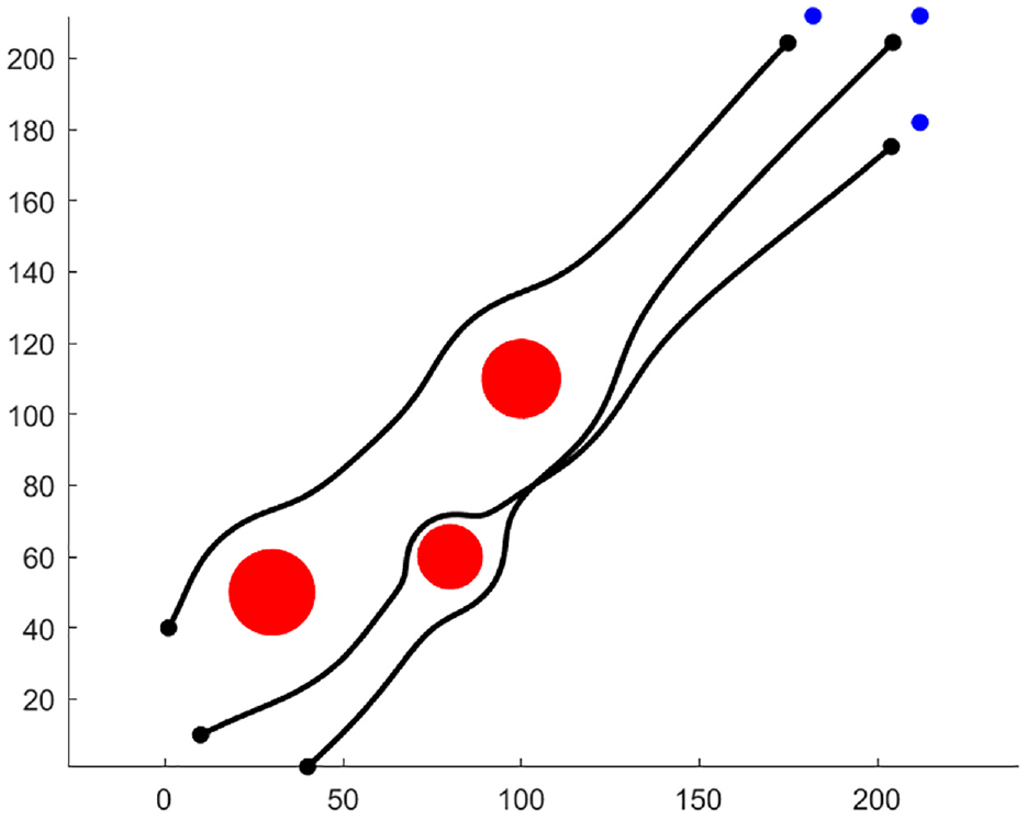
Formation flocking trajectories yielded by the USV-IFDS method.

As shown in Figure 11, equation (14) was effective in converging the velocity amplitude of individual USVs to match the velocity amplitude of the virtual formation. Figure 12 shows that the USVs did not collide with each other during FF, thereby validating the capability of the USV-IFDS method for dynamic FF.

Figure 11.

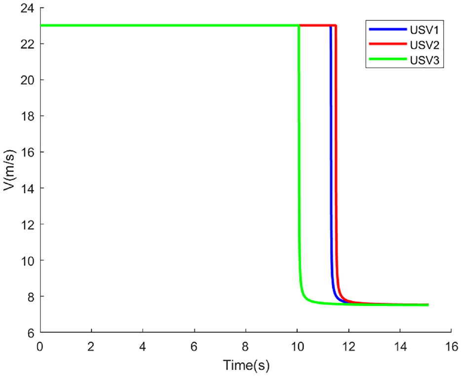
Velocity magnitude curves of flocking USVs yielded by the USF-IFDS method.

Figure 12.

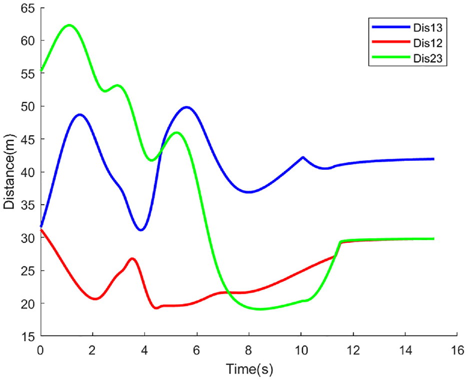
Distances between pairs of flocking USVs yielded by the USF-IFDS method.

Formation local path planning (formation OA)

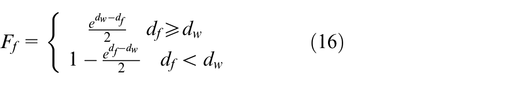
The local path planning capabilities of the USV-IFDS method were also validated by simulating a formation of three USVs with the following parameters: Starting points of USV #1, #2 and #3 were (10, 10) m, (0, 20) m and (20, 0) m, respectively; the maximum velocity was 23 m/s (approximately 45 knots); the course angle θ was 45°; the repulsion coefficient ρ_k was set to 3; the escape coefficient σ_k was set to 1; the constant C_k was set to 10; the obstacle centre was at (80, 50) m; the obstacle radius was 25 m; the initial positions of the virtual structure points for USV #1, #2 and #3 were (100, 100) m, (90, 110) m and (110, 90) m, respectively; the uniform velocity of virtual structure formation was 7.5 m/s (approximately 15 knots); the course angle θ was 45°; the distance thresholds d_vir1 and d_vir2 were 10 and 11 m, respectively; the velocity magnitude adjustment constants at distance thresholds λ_vir1 and λ_vir2 were 0.5 and 8, respectively; ρ_kf = 1; and the warning distance d_w was 13 m. Figures 13 to 15 showcase the OA performance as well as the distance between pairs of USVs.

Figure 13.

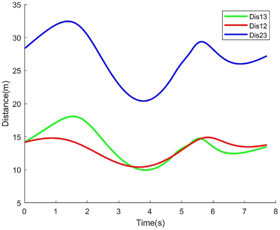
Distances between pairs of USVs during formation OA yielded by the traditional IFDS method.

Figure 14.

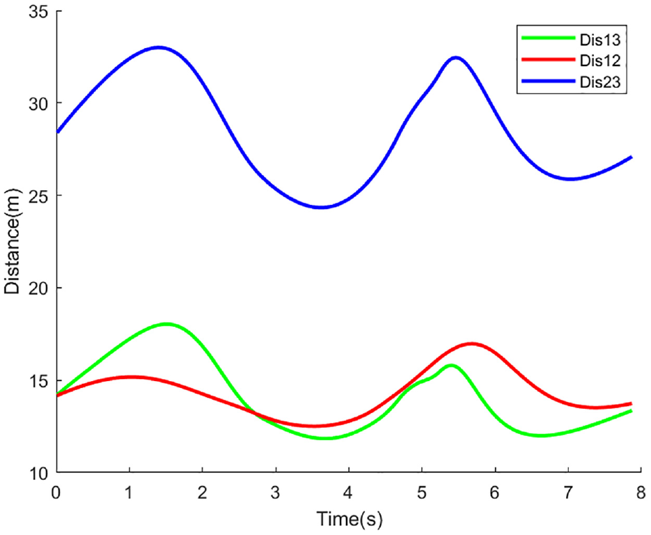
Distances between pairs of USVs during formation OA yielded by the USF-IFDS method.

Figure 15.

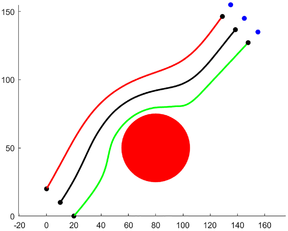
Formation OA performance of the USV-IFDS method.

Figure 13 shows that the distances between pairs of USVs calculated using the traditional IFDS method at the 4-s mark were approximately 10 m. This does not satisfy the requirements for safe navigation, because the vessels were too close to each other.

However, as shown in Figures 14 and 15, the USV-IFDS method significantly improved upon this result, effectively controlling the distances between pairs of USVs to be greater than the minimum safe distance of 13 m. This result complies with the requirements for both OA and safe navigation. Furthermore, following this phase, the individual USVs were able to successfully converge to form a coordinated formation.

Conclusion

In this study, a new path planning scheme based on disturbed flow fields is proposed for underdriven USV formation. This scheme includes solving the existing problems of IFDS in USV application and combining formation assembly and formation obstacle avoidance strategies based on the virtual structure method. The USV-IFDS scheme is an improvement of the traditional IFDS, wherein IFDS is joined the underactuated USV kinematics constraints, and through the modification of the matrix and join the constraints of the cost function, this scheme solves better the problem of local minimum. In addition, USV-IFDS uses vector and scalar decoupling in formation, which makes IFDS more suitable for formation based on the virtual structure method. It renders the formation more stable and flexible, and better overcomes the shortcomings of virtual structure formation compared with other obstacle avoidance methods. Simulation results show that the proposed formation strategy (USV-IFDS) successfully combines the advantages of IFDS and the virtual structure method, and considerably improves the formation assembly and obstacle avoidance performance of underactuated USV formation.

The simulations in this study assumed an ideal environment without considering the effects of wind and waves. Hence, in the future, we will combine the motion model of underactuated USVs in a real environment to constrain them, implement the formation architecture in a more complex real system, and further study the formation strategy.