Sage Journals: Discover world-class research

Abstract

To address the situation that the degraded system cannot be repaired as new and the degradation is accelerated after repair in engineering practice, an imperfect condition-based maintenance model is proposed based on the Gamma process by introducing the maintenance improvement factor and the accelerated degradation factor. The maintenance improvement factor describes the recovery degree of the degradation amount after imperfect maintenance, then gives a quantitative representation method of the system maintenance improvement effect and the determination method of the maximum number of imperfect maintenance. The accelerated degradation factor is combined with the geometric process to describe the accelerated degradation process of the system after imperfect maintenance. The Monte Carlo method is used to determine the optimal number of imperfect preventive maintenance decisions. Through the demonstration of calculation examples, the influence of accelerated degradation factor and maintenance improvement factor on the long-term operation maintenance rate and the optimal number of imperfect maintenance is analyzed. The results show that the model can more comprehensively describe the degradation and maintenance process of degraded systems, and it can effectively reduce maintenance cost ratio under long-term operation. It provides a certain theoretical support for formulating an economical and reasonable maintenance strategy that is more in line with the actual degradation and maintenance process in engineering practice.

Keywords

Degraded system accelerated degradation condition-based maintenance imperfect maintenance maintenance improvement

Introduction

Common mechanical equipment in daily life is a degraded system, and the degradation of the system will have a closely related impact on production and life. Maintenance is an important means to maintain the normal operation of equipment.¹ With the increasing complexity of mechanical equipment systems and the continuous improvement of safety and economic requirements, maintenance after failure can no longer meet the needs of production and life. The development of sensors and Internet of Things technology makes it possible to detect the status of equipment, and condition-based maintenance can arrange different maintenance plans and adopt different maintenance methods according to the operating status of equipment, so condition-based maintenance has attracted people’s attention. Therefore, studying the condition-based maintenance strategy of degraded systems is of great significance for improving the reliability and safety of equipment operation and reducing failure losses.

Condition-based maintenance can effectively improve the reliability of equipment so that different maintenance methods are adopted according to different conditions. But in early research on preventive maintenance, most studies used the minimum maintenance and perfect maintenance. However, in the actual maintenance process, the system is usually repaired to a certain state between “as new” and “as old,” which is imperfect maintenance.^2,3 Imperfect maintenance can repair the degradation process of the system, thus increasing the system lifetime. In the imperfect maintenance model for the degradation process, the change of degradation level before and after maintenance is generally used to describe the imperfect maintenance.⁴ The recovery degree of degradation after imperfect repair can be determined⁵ or it could be random.⁶ When the recovery degree of system degradation is determined, there are the service age reduction model and the degradation restoration model respectively.⁷ The service age reduction model believes that the service age after the maintenance will return to a certain time before the maintenance to a certain extent, and this time is the corresponding virtual service age. Accordingly, the degradation level of the system is also restored to the virtual service age. The degradation restoration model considers that after the system undergoes the imperfect maintenance, the degradation can be repaired in a certain proportion. However, some scholars believe that the maintenance recovery factor is random,⁸ so the effect of imperfect maintenance is random. When the recovery degree of the degradation level is uncertain, the Beta distribution can also be used to describe the random recovery degree of the degradation level.^9,10 In fact, as the number of imperfect maintenance increases, the impact of such maintenance will gradually diminish. The improvement in degradation level will decrease if the system continues to undergo imperfect maintenance. Therefore, it is essential to limit the number of imperfect maintenance to ensure better improvement of the degradation level after preventive maintenance.¹¹

In fact, imperfect maintenance will have multiple impacts on the system. Chen et al.¹² believe that it will have both positive and negative impacts on the system. The degradation speed of the system before and after maintenance is also affected, not just the influence of imperfect maintenance on the degradation level.¹³ In condition-based maintenance, which is based on the degradation process, it is commonly assumed that the rate of degradation of the system remains constant both before and after maintenance.^14,15 However, in actual equipment operations, the structural strength of the system gradually decreases as its age increases or maintenance is performed. This results in the phenomenon of accelerated degradation. For instance, industrial welding of metal components can shorten the crack length and extend the use time, but it will also destroy the physical mechanism of the internal material, thus accelerating the degradation rate of metal components. As a result, the system after imperfect maintenance often experiences an acceleration in its degradation process.¹⁶ Li et al.¹⁷ takes hydraulic couplers as an example to verify the existence of system degradation acceleration. Despite this, most existing strategies for preventive maintenance in degraded systems rely on perfect maintenance, and many models for imperfect preventive maintenance only take into account the changes in system state after a single instance of maintenance. For example, Van and Bérenguer¹⁸ only consider the change of degradation level after imperfect maintenance and does not consider the diminishing effect of restoration degree of degradation level after imperfect maintenance. Chen et al.¹⁹ only considers the phenomenon that the degradation process of the system accelerates with the increase of maintenance times, but does not consider the change of the degradation level after maintenance. As a result, most current condition-based maintenance models do not fully consider the changes in the imperfect system before and after maintenance.

Therefore, this paper proposes a maintenance model based on accelerated degradation after imperfect maintenance, which comprehensively considers the influence of imperfect maintenance on the degradation level and speed of the system. It describes the recovery level of the system’s degradation after imperfect maintenance through the maintenance improvement factor and uses an accelerated degradation factor to describe the acceleration of the system’s degradation process after imperfect maintenance. The model provides a robust methodology to support the formulation of realistic and reasonable maintenance strategies for degraded systems.

System description and assumptions

General assumptions

The following assumptions are used to develop the model:

Assumption 1: The system is a one-component degradation system, and its degradation level at time t can be described by a random scalar variable X(t) that can be detected. In the absence of repair or replacement operations, the degradation of the system is considered strictly incremental. At the beginning, X(0) = 0. The fault threshold is represented by X_f. When X(t) ≥X_f, the system fails, stops working, and performs corrective maintenance.

Assumption 2: The system degradation level must be periodically monitored during its operation. The monitoring accurately reflects the system’s degradation and does not interfere with its operation. The monitoring time is negligible compared to the total running time but incurs a cost for each test.

Assumption 3: Both imperfect and perfect repairs of the system are possible, and preventive maintenance strategies are employed to avoid system failures. Perfect repair restores the system degradation level to a new state; imperfect maintenance action may bring the system to any condition between as good as new and as bad as previously. Corrective maintenance is perfect maintenance.

Assumption 4: With the increase in service life and maintenance times of the system, the degradation rate of the system gradually accelerates.

Assumption 5: Ignores maintenance time and all maintenance resources required to perform preventive and are corrective maintenance always available.

Assumption 6: System degradation failure can only be found during the inspection, and then repair after failure.

Degradation model

Degradation failure is one of the main failure modes of equipment components. In the process of operation, the system experiences an increasing degradation level over time until failure due to the influence of wear, fatigue, corrosion, and crack growth, erosion, consumption, creep, swell, degrading health index, etc.²⁰ Assumption 1 posits that the degradation of the system is strictly incremental. The Gamma process, characterized by independent non-negative increments, is suitable to model gradual damage monotonically accumulating over time in a sequence of tiny increments. Mercier and Castro⁷ and Li et al. ¹⁷ are also modeled using the gamma process. Therefore, this paper adopts the Gamma process for modeling.

Considering β > 0 as a scale parameter and v > 0 as a shape parameter, the gamma density is defined as follows:

Ga (x | v, β) = \frac{β^{v}}{Γ (v)} x^{v - 1} e^{- β x} I_{(0, \infty)} (x)

(1)

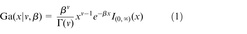
where $Γ (v) = \int_{0}^{\infty} x^{v - 1} e^{- x} d x$ is the gamma function and the indicator function is defined as: $I_{(0, \infty)} (x) = 1$ for x∈(0, +∞) and zero otherwise.

Furthermore, let v(t) be a non-decreasing, right-continuous, real-valued function for t ≥ 0, with v(0) = 0. The gamma process with shape function v(t) >0 and scale parameter β > 0 is a continuous-time stochastic process{X(t), t ≥ 0} with the following properties:

X(0) = 0,

$X (τ) - X (t) ~ Ga (v (τ - t), β)$ for τ > t ≥ 0,

$X (t)$ has independent increments.

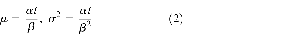
In the case that the degradation process of the system is a stationary Gamma process, v(t) = αt. Then, at time t, the expectation and variance of performance degradation are respectively:

μ = \frac{α t}{β}, σ^{2} = \frac{α t}{β^{2}}

(2)

Maintenance strategy

Condition-based maintenance strategy

The condition-based maintenance strategy mainly includes two parts: detection strategy and maintenance strategy. According to assumption 2, the length of the detection interval is represented by ΔT. Then the k-th detection time of the system is:

T_{k} = k Δ T

(3)

As shown in Figure 1, the preventive maintenance threshold of the system is $X_{p}$ , the fault threshold is $X_{f}$ , $X_{p} < X_{f}$ .

Figure 1.

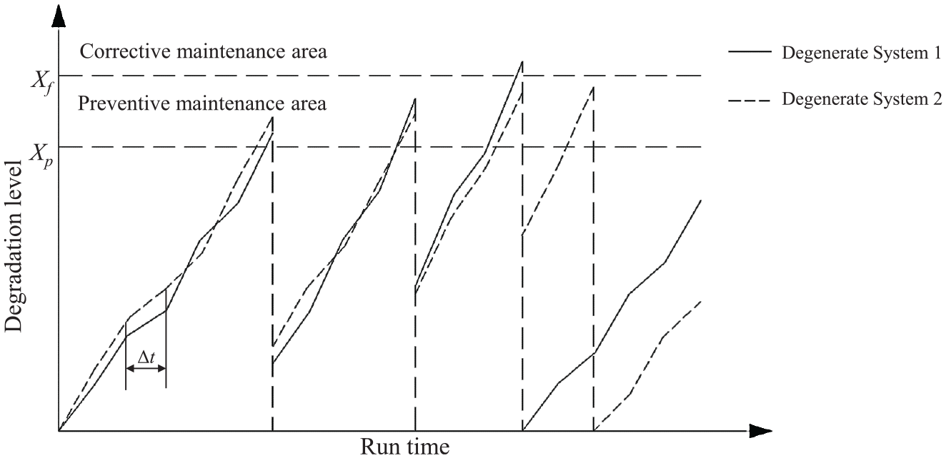
Schematic diagram of maintenance strategy.

According to the degree of degradation $X (T_{k})$ detected at the time $T_{k}$ , the specific maintenance activities are determined as follows:

(1) If the amount of degradation is less than the preventive maintenance threshold of the system, $X (T_{k}) < X_{p}$ , and the system is in normal operation, no maintenance is performed.

(2) If the degradation amount of the system is between the preventive maintenance threshold and the failure threshold, $X_{p} \leq X (T_{k}) < X_{f}$ , the system can still operate normally, but preventive maintenance is required. Preventive maintenance mainly adopts the imperfect maintenance method. According to assumptions 4 and 5, it can be seen that after several consecutive imperfect preventive maintenance, due to the accumulation of degradation amount and accelerated degradation, the imperfect maintenance effect will become worse. Therefore, after a certain number of imperfect preventive maintenance, it is changed to perfect preventive maintenance. After perfect preventive maintenance, the degradation of the system is reset to 0.

(3) If the amount of degradation exceeds the failure threshold of the system, $X (T_{k}) \geq X_{f}$ , the system fails and requires corrective maintenance. Corrective maintenance is perfect maintenance that reset the amount of degradation to 0. Since the amount of system degradation can only be detected through state detection, there is an additional cost in continuing to operate after the amount of system degradation exceeds the fault threshold until the fault is detected.

Effect of maintenance

Accelerated degradation

The degradation rate of the system is the amount of system state degradation per unit of time. According to observations, in the actual process, with the increase of service age and maintenance times, the degradation rate of the performance state of the system is not constant, but gradually accelerated. Aiming at this, this paper makes corresponding problem assumptions.

According to system assumption 5, as the system ages and undergoes more maintenance, its degradation speed accelerates, meaning the time required for its degradation level to reach X(t) from 0 decreases randomly. To model this accelerated degradation phenomenon, this paper introduces the accelerated degradation factor a and combines the geometric process with the Gamma process¹⁷ to establish an accelerated degradation process model. Then the density function of the Gamma degradation process in the nth maintenance cycle after the system undergoes n−1 imperfect maintenance is

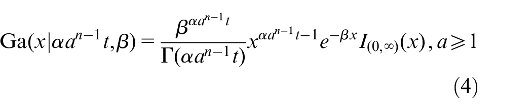
Ga (x | α a^{n - 1} t, β) = \frac{β^{α a^{n - 1} t}}{Γ (α a^{n - 1} t)} x^{α a^{n - 1} t - 1} e^{- β x} I_{(0, \infty)} (x), a \geq 1

(4)

During this period, the average degradation increment of the accelerated degradation process is

μ_{n} = \frac{α a^{n - 1} t}{β}

(5)

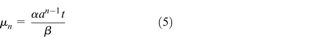
where a is the accelerated degradation parameter. When a > 1, the mean of system degradation rate μ_n will increase with the increase of n, that is, with the increase of maintenance times, the average degradation rate of the system gradually increases, which can well describe the feature that the degradation rate of the system accelerates with the gradual increase of imperfect maintenance times. In particular, when a = 1, the accelerated degradation model is the standard Gamma degradation process model.

Maintenance improvement

The amount of equipment degradation is an observable index, such as the amount of wear of the equipment, the growth of cracks, etc. Imperfect repairs give the system some degree of recovery from its degraded state before repairs. However, as the number of imperfect preventive maintenance increases, the degradation recovery effect of the equipment after maintenance becomes worse and worse. When the imperfect maintenance is not enough to restore the system to the normal operating state, the perfect maintenance will be used to restore the system to the initial state.

First, a model is built to describe maintenance improvement of imperfect maintenance. In engineering practice, it is common for a system to be restored to a state between its original condition and the state before maintenance after undergoing imperfect maintenance. To describe the impact of this type of maintenance, this paper introduces the concept of the maintenance improvement factor b.²¹ The degradation level of the system after imperfect maintenance is reduced to

X (t^{+}) = (1 - b) X (t^{-})

(6)

where b is the maintenance improvement factor; $X (t^{-})$ is the degradation level before maintenance; $X (t^{+})$ is the degradation level after maintenance. The value range of maintenance improvement factor b is $0 \leq b \leq 1$ . The larger the value is, the better the imperfect maintenance effect is. Specially, when b = 1, it is perfect maintenance; when b = 0, it is minimum maintenance. In addition, to ensure the normal operation of the system after imperfect maintenance, the maintenance improvement factor should not be less than $(X_{f} - X_{p}) / X_{f}$ .

Then, an optimization model is used to describe the deterioration of the imperfect maintenance effect with the increase of repair times. Imperfect maintenance can bring the degradation level down to a certain extent, but repeated imperfect maintenance can decrease the efficiency of degradation improvement. In other words, while imperfect maintenance repairs the degradation level of the system, frequent maintenance leads to a reduction in its improvement efficiency. To better reflect this phenomenon, the maintenance improvement factor is transformed using the power law to describe the impact of maintenance frequency on the extent of degradation. Then the improvement model of imperfect maintenance degradation can be expressed as

X (t^{+}) = (1 - b^{n}) X (t^{-})

(7)

where n is the number of imperfect maintenance, n = 1,2,3… Since the value range of b is $0 < b < 1$ during imperfect maintenance, the actual degradation improvement effect bⁿ will decrease as the number of consecutive imperfect maintenance increases.

Continuous imperfect maintenance results in a gradual reduction in the effectiveness of maintenance and a decrease in the extent of degradation improvement. Consequently, it becomes essential to incorporate a strategy where the system undergoes perfect maintenance after a certain consecutive number N of imperfect preventive maintenance cycles, so that the system can be restored as new. According to the practice, the degradation of the system after imperfect maintenance should not exceed the preventive maintenance threshold X_p, so there is

(1 - b^{N}) X (t^{-}) < X_{p}

(8)

The maximum value N_max of the number of consecutive imperfect maintenance can be obtained from Equation 8 as follows

N_{max} = \log_{b} (1 - \frac{X_{p}}{X_{f}})

(9)

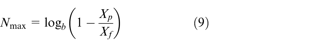
The maximum number of consecutive imperfect preventive maintenance, N, should not exceed N_max, N≤N_max. In particular, when N = 1, perfect preventive maintenance is required at the time of the first preventive maintenance.

Evaluation of maintenance policy

The long-term expected maintenance cost rate is used as the main criterion for evaluating the performance of the maintenance policy in this study.

According to the proposed maintenance strategy, the cumulative maintenance cost at time t is

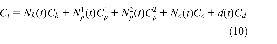
C_{t} = N_{k} (t) C_{k} + N_{p}^{1} (t) C_{p}^{1} + N_{p}^{2} (t) C_{p}^{2} + N_{c} (t) C_{c} + d (t) C_{d}

(10)

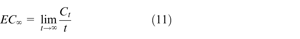
where C_t is the total maintenance cost, $C_{k}$ , $C_{p}^{1}$ , $C_{p}^{2}$ , $C_{c}$ are the costs of each inspection, each imperfect preventive maintenance, each perfect preventive maintenance, and each corrective maintenance, respectively, and $C_{d}$ is the penalty cost per unit time for continuing operation after exceeding the fault threshold; $N_{k} (t)$ , $N_{p}^{1} (t)$ , $N_{p}^{2} (t)$ , $N_{c} (t)$ are respectively the number of inspections, of imperfect maintenance, of perfect preventive maintenance, and of corrective replacement in [0, t]; $d (t)$ is the total time passed in a failed state in [0, t].

The expected rate of maintenance under long-term operation is:

E C_{\infty} = lim_{t \to \infty} \frac{C_{t}}{t}

(11)

Solution methodology

The Monte Carlo simulation method is employed in this paper to numerically solve the long-term maintenance cost rate in the maintenance model, due to its effectiveness in analyzing complex systems and solving mathematical problems through random numbers.²² The specific steps of the algorithm are presented in Figure 2.

Step 1. Set model parameters X_p, X_f, a, b, N, $N_{k} (t)$ , $N_{p}^{1} (t)$ , $N_{p}^{2} (t)$ , $N_{c} (t)$ , $C_{k}$ , $C_{c}$ , $C_{p}^{1}$ , $C_{p}^{2}$ , $C_{d}$ .

Step 2. Initialize the system. The initial running time is 0 and the initial status X(0) = 0.

Step 3. Set the detection interval to δt, use the Gamma process to generate random degradation increment, and detect the degradation level of the system at this time.

Step 4. Check whether the system is running properly. If yes, go to Step 3 to monitor the degradation level of the system. If not, go to the next step.

Step 5. Evaluate whether the degradation level exceeds the fault threshold or not. If the degradation level exceeds the fault threshold, carry out corrective maintenance, calculate the fault running time, increase the number of corrective maintenance N_c = N_c + 1, and restore the system degradation level and degradation speed to the initial state after corrective maintenance. Otherwise, the system undergoes imperfect preventive maintenance and proceeds to the next step.

Step 6. Calculate the number of continuous imperfect preventive maintenance. If the number of continuous imperfect preventive maintenance is less than N, the imperfect preventive maintenance is carried out. The number of imperfect preventive maintenance is $N_{p}^{1}$ = $N_{p}^{1}$ +1, and the degradation level after imperfect maintenance is improved. Otherwise, perfect preventive maintenance is required for the system. The number of perfect preventive maintenance is $N_{p}^{2}$ = $N_{p}^{2}$ +1. After perfect preventive maintenance, the degradation level and degradation speed of the system return to the initial state.

Step 7. Calculate the total cost.

Step 8. Check whether the system running time reaches the set running time. If not, return to Step 3 to continue running. Otherwise, end the operation and output the long-term operation maintenance cost rate.

Figure 2.

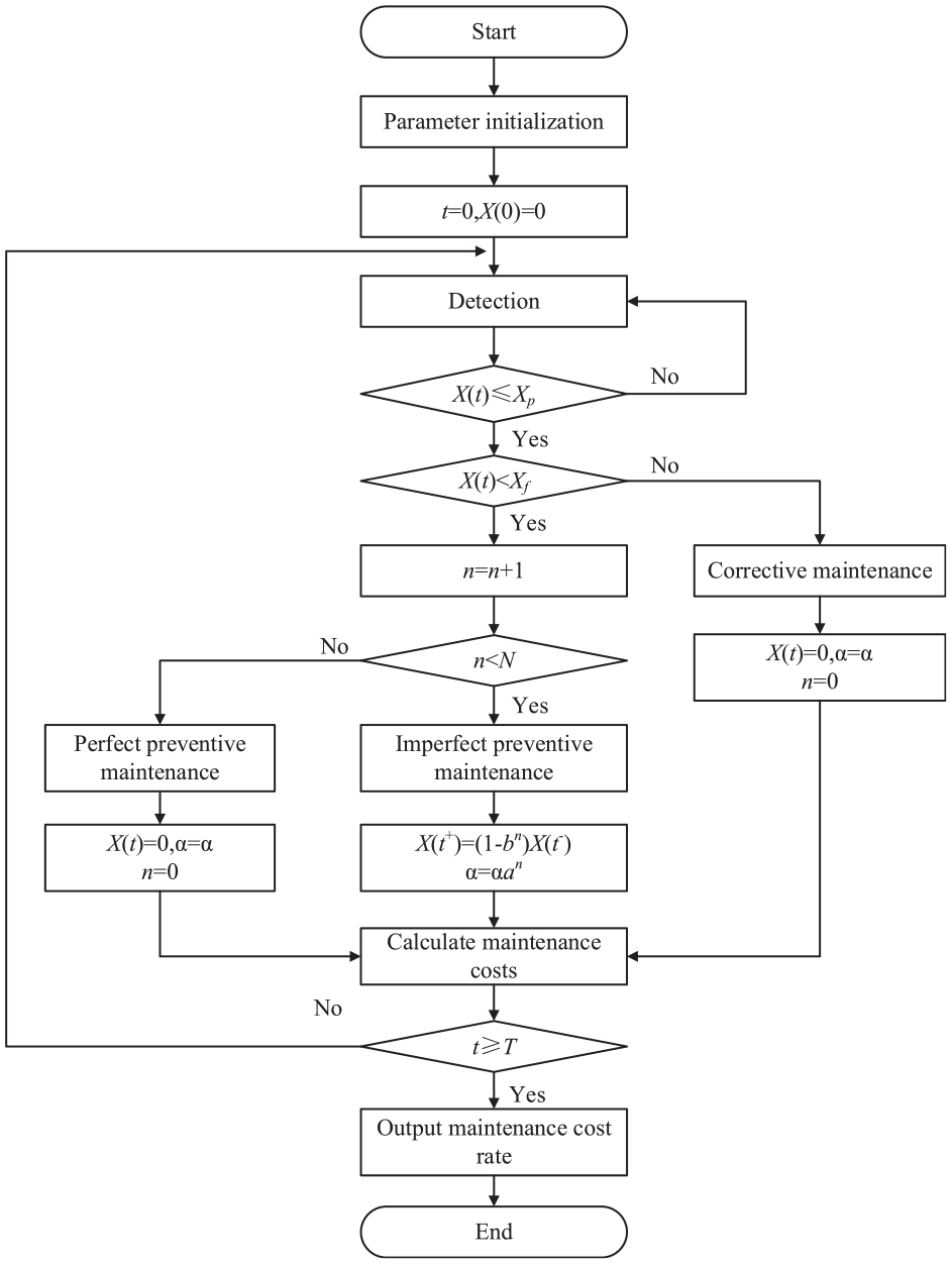
Monte Carlo simulation process.

Numerical example

The purpose of this section is to show how the proposed maintenance model can be used in the maintenance optimization of deteriorating systems through a simple example.

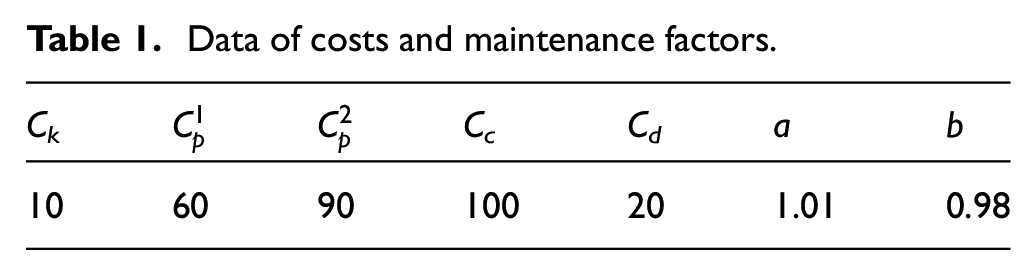
To analyze and verify the validity of the model without loss of generality, assume a single unit degenerate system whose degradation process follows a Gamma process with scale parameter α = 1 and shape parameter β = 1. The system periodically detects the system status with period δt = 1, the system fault threshold $X_{f}$ = 10, and the preventive maintenance threshold $X_{p}$ = 6, when the preventive maintenance threshold is exceeded but no failure occurs, imperfect maintenance is adopted. Table 1 reports the data related to inspection, maintenance costs, penalty costs, and the maintenance factor. According to Formula (9), N_max = 45. After several consecutive imperfect preventive maintenance, the maintenance effect gradually deteriorates, so the value of N should be smaller. To verify the feasibility of the Monte Carlo simulation algorithm, N = 5.

Table 1.

Data of costs and maintenance factors.

C_k	$C_{p}^{1}$	$C_{p}^{2}$	C_c	C_d	a	b
10	60	90	100	20	1.01	0.98

To evaluate the mean maintenance cost per unit of time, a very large number of simulation realizations are done. Through Monte Carlo simulation, the simulation of continuous running 10,000 h. Run 1000 times respectively, and the results of 10 times are shown in Figure 3. It can be seen from Figure 3 that the expense rate of long-term operation cost has convergence. By calculating the average value of 1000 times of operation, the long-term operation rate converges to 20.07, indicating that this calculation method is feasible.

Figure 3.

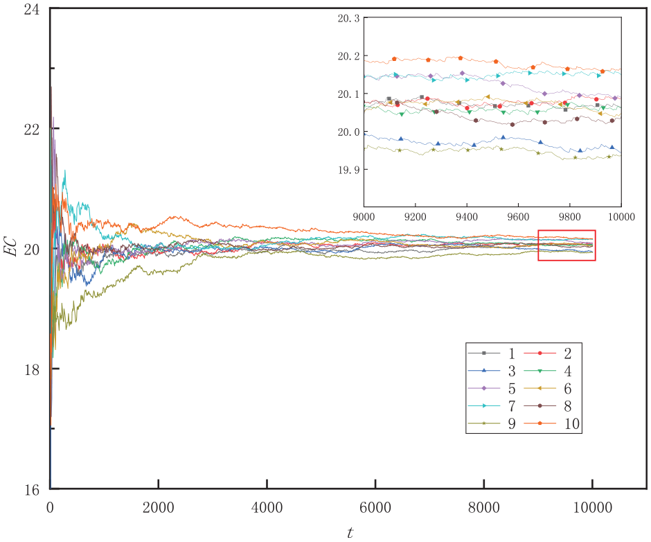
Convergence of simulation results.

After several consecutive imperfect preventive maintenance, the maintenance effect gradually deteriorates, which makes the imperfect preventive maintenance ineffective. Therefore, the convergence value of the long-term operation maintenance cost rate from 1 to N_max is calculated respectively, as shown in Figure 4 shown. As can be seen from the figure, the maintenance cost rate decreases first and then increases with the increase of the number of imperfect maintenance decisions, and there is an optimal number of imperfect maintenance decisions. When N = 1, the system adopts perfect preventive maintenance. Under this maintenance strategy, the long-term operation maintenance cost rate is about 22.92, which is higher than most imperfect preventive maintenance strategies. With the increase of N, when N = 6, the long-term operation maintenance cost rate reaches the lowest, which is about 20.06. When N continues to increase, the maintenance cost rate begins to increase gradually. Therefore, when N = 6, the maintenance strategy under this condition is optimal, and the long-term operation maintenance expense rate is reduced by about 12.5% compared with perfect preventive maintenance.

Figure 4.

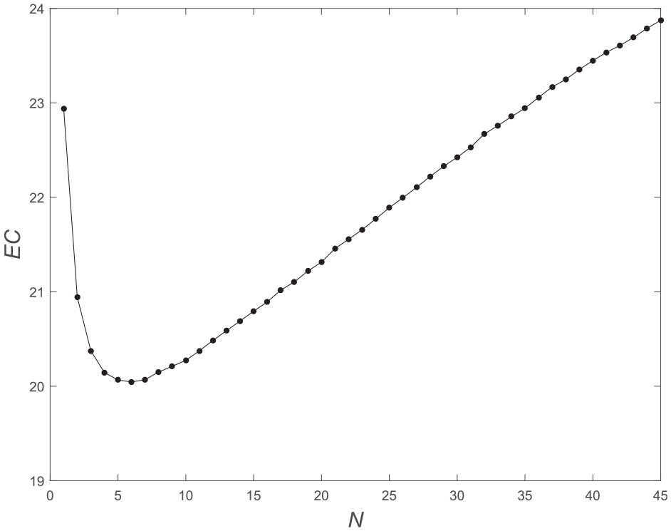
Changes in maintenance expense rate under different times of imperfect maintenance decisions.

Sensitivity analysis

Based on actual maintenance experience, the rate of accelerated degradation and the effectiveness of maintenance improvements can significantly affect the maintenance strategy. Thus, the following analysis focuses on the effect of the accelerated degradation factor and the maintenance improvement factor of imperfect maintenance on the long-term operating maintenance rate and the optimal number of imperfect maintenance. This will provide valuable insights into how these factors can influence the maintenance decision-making process.

The impact of the accelerated degradation factor and maintenance improvement factor on the long-term operation maintenance rate is analyzed in the first step. Figure 5 shows the change in maintenance cost rate under different parameters by varying the values of accelerated degradation factor and maintenance improvement factor when N = 5. The results indicate that, for the same number of imperfect maintenance, a higher accelerated degradation factor leads to a higher long-term maintenance cost ratio of imperfect maintenance when the maintenance improvement factor is constant. Conversely, when the accelerated degradation factor is constant, a larger maintenance improvement factor results in a lower long-term maintenance cost ratio.

Figure 5.

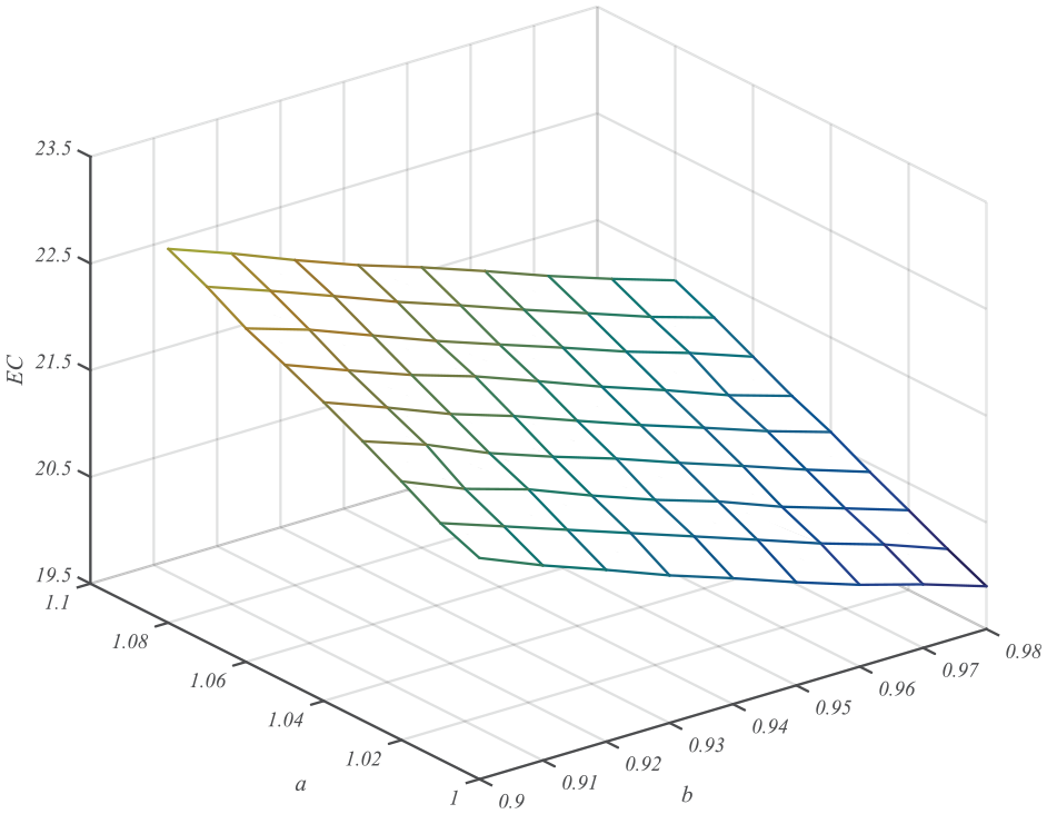
Influence of maintenance improvement factor and accelerated degradation factor on maintenance cost ratio.

Based on the analysis of the system’s degradation and maintenance processes, it can be observed that when the number of maintenance interventions is fixed and the maintenance improvement factor remains constant, an increase in the accelerated degradation factor results in a higher degradation rate of the repaired system, shorter normal operation time, and subsequently a higher maintenance cost rate. On the other hand, when the accelerated degradation factor is constant, after the same number of imperfect maintenance, the larger the maintenance improvement factor is, the more obvious the improvement effect of the repaired degradation level is, so that the repair can be restored to a better state and the normal operation time is longer, so the maintenance cost rate is lower.

When the maintenance improvement factor b and imperfect maintenance times N have different values, the change in long-term operation maintenance cost rate is shown in Figure 6. As shown in the figure, there is an optimal number of continuous imperfect maintenance decisions, and the maintenance cost initially decreases and then rises as the number of imperfect maintenance increases, while the maintenance improvement factor is held constant. At the optimal number of imperfect maintenance decisions, the long-term operation maintenance cost rate is the lowest. For example, when b = 0.96 and N = 3, the maintenance cost rate is 20.59, which is lower than the maintenance cost rate of the perfect preventive maintenance strategy when N = 1. Similarly, when N = 5, the maintenance cost rate is at its lowest, which is 20.47, lower than the rate when N = 1. However, when N = 7, the maintenance cost rate increases slightly to 20.68, but it is still lower than the maintenance cost rate of the perfect preventive maintenance strategy when N = 1. Therefore, the imperfect maintenance strategy can effectively reduce the maintenance cost ratio and is an effective preventive maintenance strategy. Moreover, it is observed that the optimal number of imperfect maintenance decisions tends to increase with the maintenance improvement factor. For instance, when b = 0.9, the optimal number of maintenance decisions N = 3; When b =0.96, N = 5.

Figure 6.

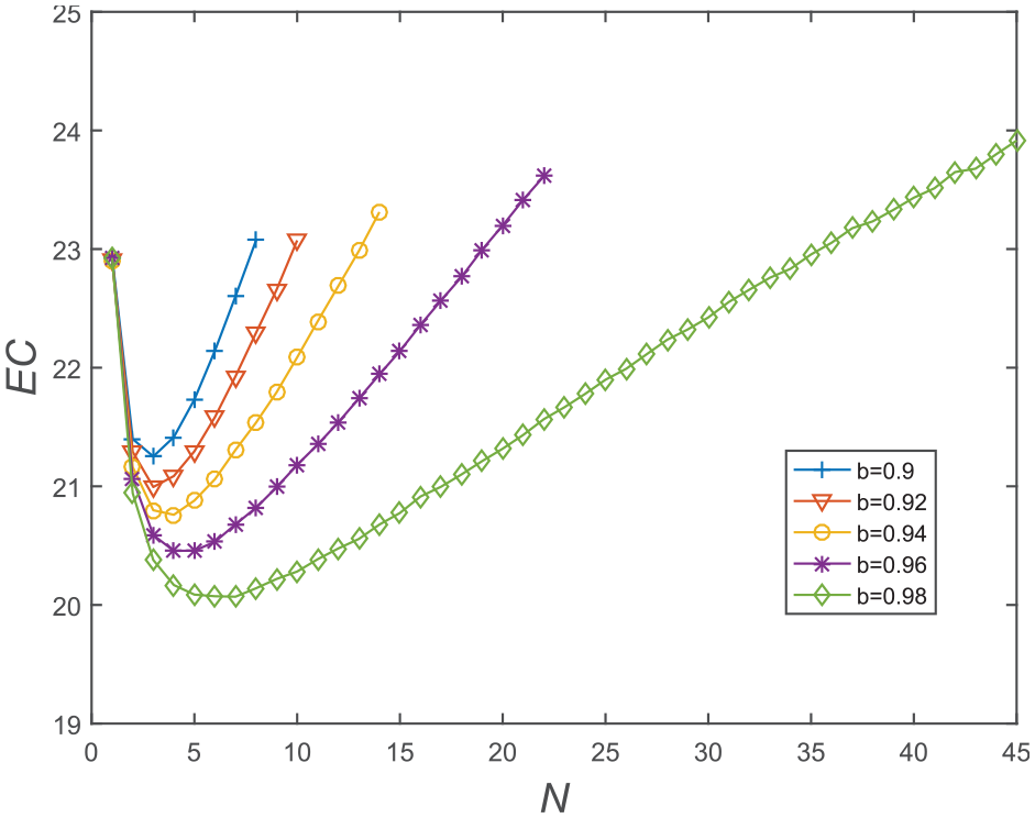
Influence of maintenance improvement factor on optimal decision times.

The degradation and maintenance analysis of the system shows that the initial imperfect maintenance decisions can restore the system to a better state, leading to longer normal operation times and lower costs compared to perfect maintenance. This results in a lower maintenance cost rate overall, indicating the effectiveness of the imperfect maintenance strategy. As the number of imperfect maintenance continues to increase, the maintenance effect of imperfect maintenance gradually decreases, so the actual degradation level repair degree of the system after imperfect maintenance gradually decreases, and the normal operation time of the system after maintenance shortens. Consequently, when N continues to increase, the maintenance cost rate begins to increase gradually. Therefore, the imperfect maintenance strategy has the optimal decision time. In addition, the larger the maintenance improvement factor is, the better the maintenance effect is. Appropriately increasing the maintenance times can still keep the system running for a longer time and reduce the maintenance cost rate. Therefore, the optimal number of imperfect maintenance shows an increasing trend. Furthermore, when the number of imperfect preventive maintenance is not limited, that is, N is infinite, with the unlimited increase of the actual number of imperfect maintenance, the maintenance cost rate gradually increases, so the maximum number of imperfect maintenance should be limited in the actual repair process. In the actual maintenance process, to ensure the normal operation of the system and reduce the maintenance cost rate, the maintenance improvement effect should be between (X_f– X_p)/X_f and 1, and the greater the improvement effect, the better. At the same time, it is necessary to limit the number of imperfect maintenance and determine the optimal number of imperfect maintenance according to the actual maintenance improvement situation.

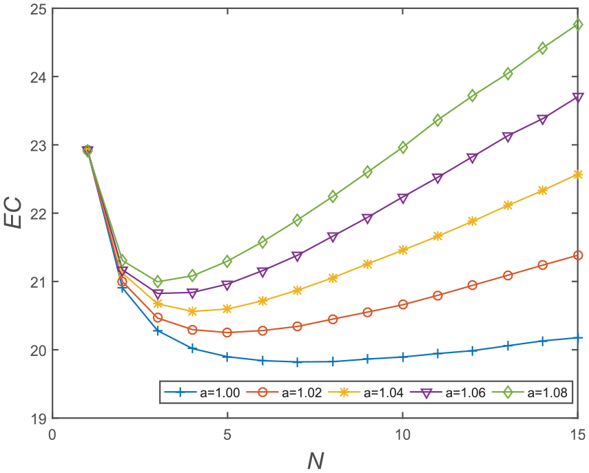
When the accelerated degradation factor a and the number of imperfect maintenance are of different values, the change in long-term operation maintenance cost rate is shown in Figure 7. As can be seen from the figure, when a = 1.00, there is no accelerated degradation of the system. When only imperfect maintenance is considered, the maintenance cost rate of the system for long-term operation is significantly lower than that under accelerated degradation. Therefore, the accelerated degradation process of the system leads to an increase in maintenance costs. With the increase of the accelerated degradation factor, the optimal number of imperfect maintenance has a trend of decreasing. For example, when a = 1.00, the optimal number of imperfect maintenance N = 7; When a = 1.04, the optimal number N = 4; When a = 1.08, the optimal number N = 3. Therefore, ignoring the accelerated degradation caused by imperfect maintenance will affect the formulation of optimal maintenance strategies.

Figure 7.

Influence of accelerated degradation factor on optimal decision times.

Through the analysis of the system degradation process, it is observed that when the accelerated degradation speed is constant, with the gradual increase of maintenance times, the improvement effect of the system gradually decreases and the actual degradation speed of the system significantly accelerates. As a result, the normal operation time after maintenance gradually shortens. Moreover, under the same conditions, the larger the accelerated degradation speed is, the higher the maintenance cost ratio is. To control the increase of the degradation speed and reduce the maintenance cost rate, the number of imperfect maintenance should be reduced. Therefore, the optimal number of maintenance shows a decreasing trend with the increase of the accelerated degradation factor. It is evident that the accelerated degradation process of the system significantly affects the maintenance cost rate of the system. If the accelerated degradation is not considered in the maintenance process, it will also affect the determination of the optimal number of imperfect maintenance. To formulate a reasonable maintenance strategy and reduce the maintenance cost rate, it is essential to pay attention to equipment maintenance during the use of the degraded system to reduce the accelerated degradation rate of the system. Furthermore, it is crucial to consider the influence of accelerated degradation when formulating the maintenance strategy to reasonably estimate the accelerated degradation rate of the system.

Conclusion

(1) In this paper, an imperfect condition-based maintenance model for the accelerated degradation system is proposed. The model considers both the improvement effect of system degradation after maintenance and the influence of degradation rate on maintenance decisions. It is a new condition-based maintenance decision-making model. This model can more comprehensively describe the degradation and maintenance process of degraded systems in engineering practice.

(2) The system degradation process is described based on the Gamma process, the calculation example is used for analysis and verification, and the solution method for the optimal number of imperfect preventive maintenance is given. Additionally, the optimal maintenance strategy is analyzed under different maintenance and degradation processes, offering a theoretical basis for formulating cost-effective and reasonable maintenance strategies for degraded systems.

Footnotes

Declaration of conflicting interests

The author(s) declared no potential conflicts of interest with respect to the research, authorship, and/or publication of this article.

Funding

The author(s) disclosed receipt of the following financial support for the research, authorship, and/or publication of this article: Project supported by the National Key Research and Development Program of China (No.2019YFB1707303).

ORCID iD

Jintao Chen

References

Noman

Nasr

ESA

Al-Shayea

, et al. Overview of predictive condition based maintenance research using bibliometric indicators. J King Saud Univ Eng Sci 2019; 31(4): 355–367.

Zheng

, et al. Remaining useful life prognostic for the stochastic degradation device subject to imperfect maintenance. Acta Electon Sin 2017; 45(7): 1740.

Pei

Wang

, et al. A new remaining useful life estimation method for equipment subjected to intervention of imperfect maintenance activities. Chin J Aeronaut 2018; 31(3): 514–528.

Voisin

Levrat

, et al. A proactive condition-based maintenance strategy with both perfect and imperfect maintenance actions. Reliab Eng Syst Saf 2015; 133: 22–32.

Zhao

, et al. Condition-based maintenance and optimizing strategy with imperfect repair for deep-water pipeline. Tianjin Daxue Xuebao 2016; 49(09): 902–906.

Zhang

, et al. Optimization of condition-based maintenance for degradation systems under imperfect maintenance. Acta Aeronaut et Astronaut Sin 2013; 34(2): 316–324.

Mercier

Castro

. Stochastic comparisons of imperfect maintenance models for a gamma deteriorating system. Eur J Oper Res 2019; 273(1): 237–248.

Omshi

Grall

. Replacement and imperfect repair of deteriorating system: Study of a CBM policy and impact of repair efficiency. Reliab Eng Syst Saf 2021; 215: 107905.

Cheng

Zhou

. Integrated production, quality control and condition-based maintenance for imperfect production systems. Reliab Eng Syst Saf 2018; 175: 251–264.

10.

Liao

Elsayed

Chan

. Maintenance of continuously monitored degrading systems. Eur J Oper Res 2006; 175(2): 821–835.

11.

Liu

Xie

, et al. An imperfect maintenance policy for mission-oriented systems subject to degradation and external shocks. Comput Ind Eng 2016; 102: 21–32.

12.

Chen

Gong

, et al. Imperfect maintenance policy considering positive and negative effects for deteriorating systems with variation of operating conditions. IEEE Trans Autom Sci Eng 2018; 15(2): 872–878.

13.

Chuang

Ningyun

Bin

, et al. Condition-based maintenance optimization for continuously monitored degrading systems under imperfect maintenance actions. J Syst Eng Electronics 2020; 31(4): 841–851.

14.

Yang

Zhao

. Condition-based maintenance strategy for critical ship components based on performance degradation. J Harbin Eng Univ 2020; 41(04): 613–618.

15.

Do Van

Bérenguer

. Condition-based maintenance under an imperfect repair policy for a deteriorating production system. In: 7th International conference on modelling in industrial maintenance and reliability (MIMAR 2011), Cambridge, UK, 2011, p.6.

16.

Cheng

Zhou

, et al. Modeling condition-based maintenance and replacement strategies for an imperfect production-inventory system. Proc IMechE, Part B: J Engineering Manufacture 2018; 232(10): 1858–1871.

17.

Cheng

Liu

. Accelerated degradation system model based on gamma process and its optimal condition-based maintenance strategy. Comput Integr Manuf Syst 2013; 19(11): 2922–2927.

18.

Van

Bérenguer

. Condition-based maintenance with imperfect preventive repairs for a deteriorating production system. Qual Reliab Eng Int 2012; 28(6): 624–633.

19.

Chen

Jiang

, et al. Optimization of condition-based maintenance strategy for single-unit accelerated degrading systems. J Syst Eng Electronics 2020; 42(3): 613–619.

20.

Lin

Tang

Ning

, et al. Condition-based maintenance strategy for dynamic performance detection based on Wiener process. J Ordnance Equip Eng 2021; 42(7): 40–45.

21.

Rahimikelarijani

Hamidi

Mohassel

, et al. Imperfect condition-based maintenance strategy for a deteriorating rail track system with multiple competitive failure modes. J Transp Eng A Syst 2020; 146(9): 04020088.

22.

Niu

Guo

, et al. Preventive maintenance period decision for elevator parts based on multi-objective optimization method. J Build Eng 2021; 44: 102984.

Research on imperfect condition-based maintenance strategy based on accelerated degradation process

Abstract

Keywords

Introduction

System description and assumptions

General assumptions

Degradation model

Maintenance strategy

Condition-based maintenance strategy

Effect of maintenance

Accelerated degradation

Maintenance improvement

Evaluation of maintenance policy

Solution methodology

Numerical example

Sensitivity analysis

Conclusion

Footnotes

Declaration of conflicting interests

Funding

ORCID iD

References