
Abstract
In this article, we consider an imperfect production-inventory system which produces a single type of product to meet the constant demand. The system deteriorates stochastically with usage and the deterioration process is modeled by a non-stationary gamma process. The production process is imperfect which means that the system produces some non-conforming items and the product quality depends on the degradation level of the production system. To prevent the system from deteriorating worse and improve the product quality, preventive maintenance is performed when the level of the system degradation reaches a certain threshold. However, the preventive maintenance is imperfect which cannot restore the system as good as new. Hence, the aging system will be replaced by a new one after some production cycles. The preventive maintenance cost, the replacement cost, the production cost, the inventory holding cost and the penalty cost of lost sales are considered in this article. The objective is to minimize the total cost per unit item which depends on two decision variables: the preventive maintenance threshold and the time at which the system is replaced. We derive the explicit expression of the total cost per unit item and the optimal joint policy can be obtained numerically. An illustrative example and sensitivity analysis are given to demonstrate the proposed model.
Keywords
Introduction
For production-inventory systems, the economic production quantity (EPQ) model is applied to reduce the production- and inventory-related costs. In the earliest EPQ models, a common limited assumption is that machines never fail during a production run. However, most production systems suffer increasing wear or deteriorate with usage or aging process. Eventually, they fail from this deterioration without preventive maintenance (PM). The machine breakdowns and corrective maintenance have a great influence on production planning and inventory management. Therefore, an appropriate PM strategy should be selected to improve the system reliability with minor sacrifices during production run.
The production models with PM have been intensively studied by some researchers. Meller and Kim 1 considered a production system and assumed that periodic PM can decrease the production operation’s failure rate in the long run. They used an embedded absorbing Markov chain analysis to determine the optimal inventory level which triggers the PM. Abboud 2 considered a single machine production-inventory system and assumed that the times-to-failure and the repair times are geometrically distributed. A Markov chain model was developed and an efficient algorithm was proposed to find the economic manufacturing quantities. Chung et al. 3 extended the above model by considering the deteriorating items with stochastic machine unavailable time and shortage. Widyadana and Wee 4 developed two EPQ deteriorating item models of uniform distribution and exponential distribution of corrective and maintenance times. Wee and Widyadana 5 developed an EPQ model with stochastic PM time and rework process. Recoverable items (defined as items that do not meet quality standards but can be reprocessed) are reprocessed by the last in first out (LIFO) rule. Then, Wee and Widyadana 6 revisited the above model using the first in first out (FIFO) rule for rework process. With the development of sensor and information technologies, the degradation level of systems can be monitored to estimate the systems’ state and facilitate the prediction of failures.7,8 Hence, condition-based maintenance (CBM) has been widely used in maintenance area due to its effectiveness and efficiency. However, few researches have been done to investigate the joint model for EPQ and CBM. Jafari and Makis 9 studied joint optimization of EPQ and CBM. The problems are formulated and solved in the semi-Markov decision process framework. Peng and Van Houtum 10 proposed a model to determine the production of lot-sizing and CBM policy by assuming a continuous degradation process of the system. Renewal theory is employed to compute the average long-run cost rate.
Note that the PM in the above literature is assumed to be perfect, that is, it can restore the machine to the state as good as new. However, in practice, it is not always the case. For more realistic, some researchers considered imperfect PM in production-inventory system models. Sheu and Chen 11 developed an integrated model for the joint optimization of EPQ and level of PM. They assumed that after performing PM, the aging of the system is reduced in proportion to the PM level. Wang et al. 12 extended the model by considering inspections which are used to see whether the process is in control. El-Ferik 13 assumed that the age-based PM is imperfect and the machine will be replaced at the Nth maintenance. The objective was to obtain the optimal PM interval and replacement policy such that the long-run average cost rate is minimized. Ouaret et al. 14 simultaneously determined the optimal production rate and replacement policy for a failure-prone manufacturing system by considering the imperfect maintenance. Semi-Markov processes and numerical methods were used to model the dynamics of the system and obtain the optimal control policies. Cheng et al. 15 studied a production system which consists of two machines and one buffer. The machine tends to deteriorate faster as the number of maintenance increases. An integrated model was developed for the joint determination of buffer size and PM interval. More recently, Cheng et al. 16 employed geometric process to describe the effects of imperfect maintenance. The aging machine will be replaced after N failures. An algorithm is proposed to obtain the optimal buffer size and replacement policy.
It is well known that the deterioration process influences not only the reliability of the production system but also the quality of products. Indeed, the machine state plays an important role in controlling the quality of produced items. 17 Ben-Daya 18 developed an EPQ model linking quality and PM. The production process may shift from “in-control” state to “out-of-control” state after random period of time and then produces some non-conforming items. The author jointly determined the EPQ and PM level and proved that performing PM can reduce the quality-related costs. Peter Chiu et al. 19 concerned with the algebraic derivation for the production lot-sizing problem considering random defective rate, rework process and backlogging. Radhoui et al. 17 studied a joint quality control and PM policy for an imperfect production system. The PM level was defined as the proportion of non-conforming items produced. Simulation and experimental design were used to determine the optimal buffer size and PM level simultaneously. Yang and Zeng 20 proposed an equipment maintenance policy by integrating periodic equipment inspection and product quality control. Maintenance action is chosen based on the inspection result of the product quality shift and equipment degradation state. The optimal maintenance policy is obtained by genetic algorithm. Sana 21 considered a production-inventory model in an imperfect production process with time-varying demand. The author assumed that the unit production cost is a function of product reliability parameter and production rate which are two decision variables of the model. The optimal solutions are obtained using the Euler–Lagrange method. Pal et al. 22 assumed that non-conforming items are produced in the both “in-control” and “out-of-control” states. The probability of non-conforming items produced is smaller in the “in-control” state than in the “out-of-control” state. After regular production run time, the non-conforming items are reworked and the PM is performed. The optimal buffer inventory and production run time are obtained to minimize the unit production cost. Other production-maintenance models considering product quality can be seen in Chouikhi et al., 23 Liao, 24 and Tsao 25 and Jeang. 26
In the literature mentioned above, the states of production systems are generally divided into two classes: “in-control” state and “out-of-control” state. When the system stays in the “in-control” state, no or less non-conforming items are produced. While in the “out-of-control” state, the system produces more non-conforming items. This assumption reflects the fact that the degradation of systems influences the product quality. However, in practice, only two states may not be able to describe the degradation level of the system accurately. For example, the tool wear is a gradual deteriorating process. According to ISO 3685,
27
based on the size of flank wear monitored (denoted by
In this article, CBM and replacement strategies are proposed for a production-inventory system taking into account degradation-level-dependent quality. The production system deteriorates gradually, and its deterioration process is modeled by gamma process which is widely used in maintenance models for deteriorating systems. 28 The proportion of non-conforming items depends on the system’s degradation level monitored, that is, the more non-conforming items are produced when the system deteriorates to a higher level. PM actions are performed to control the system degradation and improve the product quality when the deterioration level reaches the threshold which is a decision variable of the model. Further assumed that the PM is imperfect, that is, it cannot bring the system to its initial state. Consequently, the aging system will be replaced after N maintenance actions, where N is another decision variable of the model. Our aim is to minimize the total cost per unit item produced consisting of PM, replacement, production, inventory holding and lost sales costs. The maintenance optimization model is formally developed and the optimal joint strategy is obtained numerically. The rest of this article is organized as follows. Section “Assumptions and notations” presents model assumptions and notations used. Section “Model description” provides a detailed model description. Section “Formulation of the model” is dedicated to the derivation of the explicit expression of the total cost per unit item. Section “An illustrative example and discussions” gives an illustrative example to obtain the optimal joint strategy numerically and carry out some sensitivity analysis. Finally, conclusions are drawn in the last section.
Assumptions and notations
The following assumptions and notations are used to develop the model.
Assumptions
A1. At the beginning, a new production system is installed which produce one type of product to meet the constant demand.
A2. The production system deteriorates with use and age and its degradation behavior is modeled by a stochastic process. The system failure occurs when the degradation level exceeds the predetermined threshold.
A3. The production process is imperfect, that is, the system produces some defective or non-conforming items which cannot be reworked and are scrapped. In addition, the proportion of non-conforming items depends on the degradation level of the system, that is, the system produces non-conforming items at a higher rate as the degradation level increases.
A4. The system is monitored continuously and perfectly, which reveals the true degradation level in real time. The PM is performed when the degradation level reaches the PM threshold. It is assumed that the PM is imperfect which cannot restore the system to the state as good as new. More details are available in the following section.
A5. Since the PM is imperfect, the production system will be replaced by an identical new one after some production cycles.
A6. The production rate of conforming items is greater than the demand rate. The initial inventory level is zero. In this article, the no-resumption (NR) policy 29 is adopted which means that after the PM or replacement, a new production cycle starts when the on-hand inventory is depleted.
A7. When demand is greater than the stock during PM time, shortage occurs. We assume shortage items are lost sales.
A8. The model is studied over infinite planning horizon.
Notations
P production rate of the system;
D constant demand rate;
a ratio of the geometric process;
N decision variable which means the system will be replaced after N production cycle;
Model description
Deterioration modeling
Consider a production system which deteriorates due to usage and age. The degradation evolution is modeled by a stochastic process. Let
where
The average deterioration rate is
where
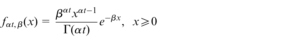
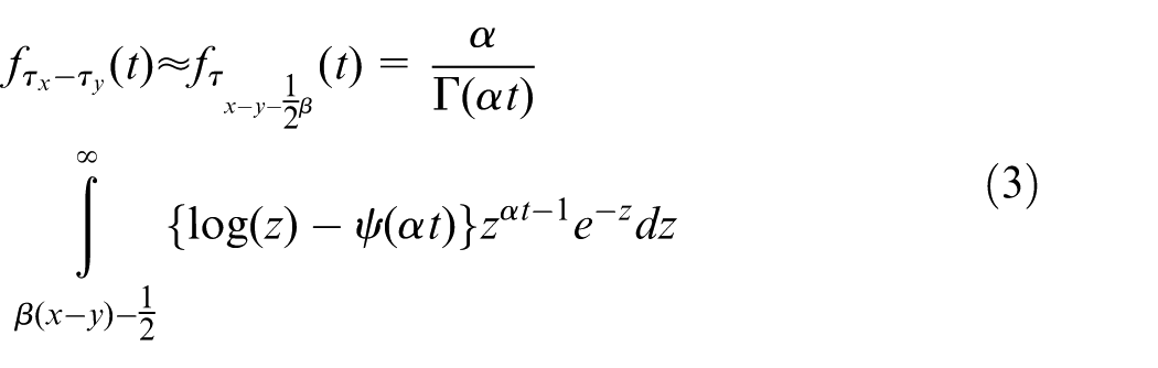
The density function
where
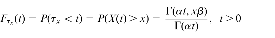
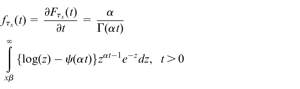
Let
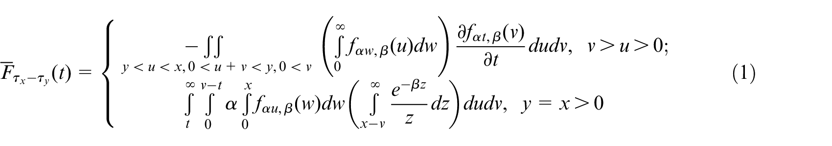
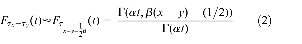
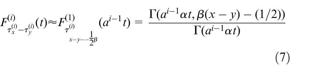
Since expression (1) is too complicated for numerical computations, Bérenguer et al.
31
gave an approximation of the distribution function of
Imperfect production process
In this article, the production process is assumed to be imperfect, that is, some produced items may be non-conforming. Furthermore, it is reasonable to assume that the rate of non-conforming items depends on the degradation level of the system, that is, the rate increases as the degradation level increases. Assume that there are M thresholds of the deterioration process, namely,
Imperfect PM
According to assumption A4, a CBM is applied to this production system based on the information obtained from continuous monitoring. If the degradation level
Here, we assume that the distribution function of the degradation state immediately after the ith PM
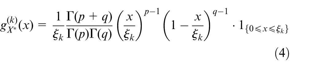
where the parameters
Remark 1
From the definition of Beta distribution, if the PM threshold is
In addition, the system is assumed to tend to deteriorate faster as the number of PM increases. This phenomenon is common in practice. For example, the amplitude of the hydraulic coupler can reflect its deterioration states and the growth of the amplitude is accelerated after each repair (see the data in Tan et al. 33 ). Here, we employ the accelerated deteriorating gamma process (ADGP) to model this stochastic process which is first introduced by Cheng et al. 15
The ith production cycle is referred to as the time duration from the beginning of the production after the (i − 1)th PM until the beginning of the ith PM action or replacement. Let
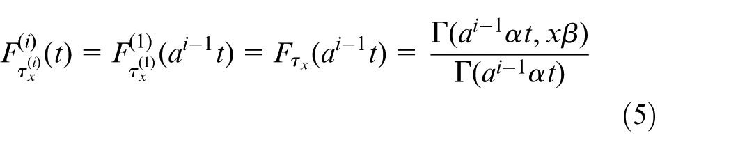
where a is the ratio of geometric process and
Consequently, the density function
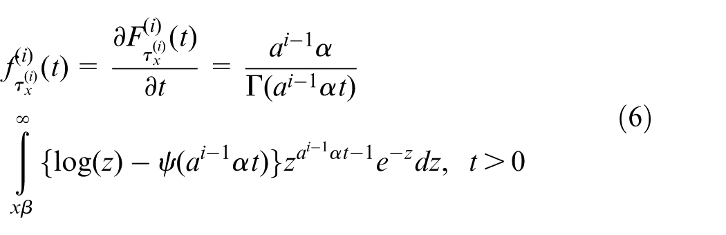
Similar to expressions (2) and (3),
Remark 2
According to expression (5), the shape parameter and the scale parameter of the gamma process after the ith maintenance are
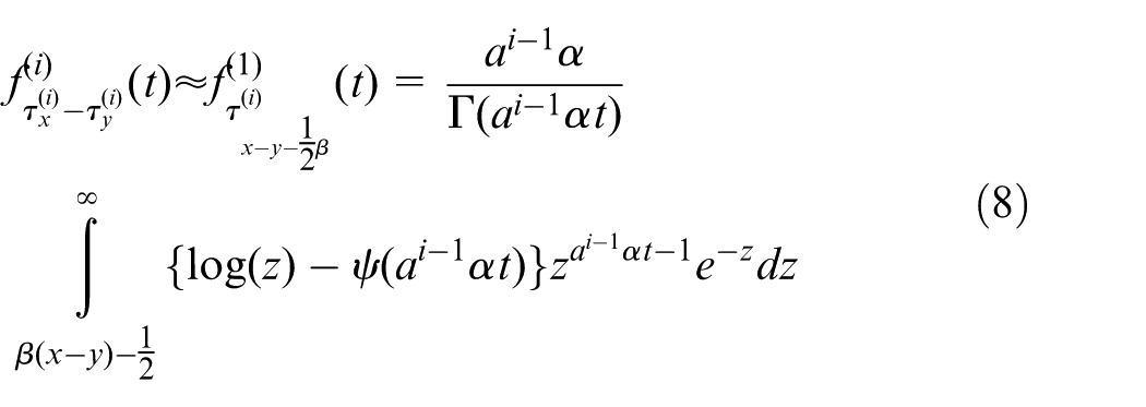
By assuming that the PM threshold is
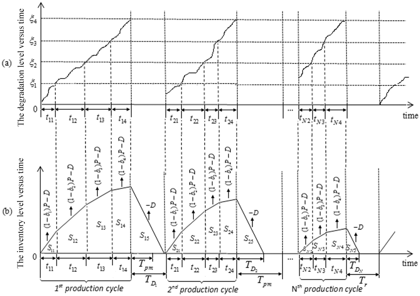
The system degradation level and inventory level versus time
Formulation of the model
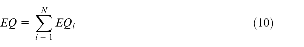
According to renewal reward theorem, the total expected quantity of conforming items produced can be derived by dividing the total expected cost per renewal cycle to the total expected quantity produced in a renewal cycle as the following

Expected total quantity of conforming items produced in a renewal cycle
Let
According to assumption A3, the production rate of non-conforming items depends on the system’s degradation level, that is, the rate is
where
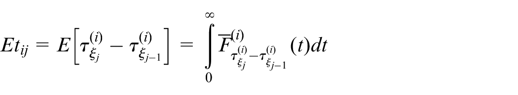
Based on the above discussion, we have the following
When
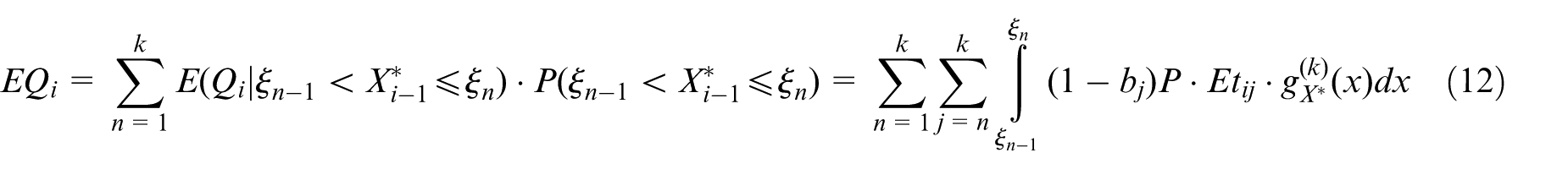
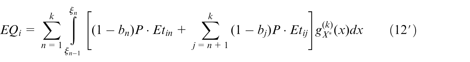
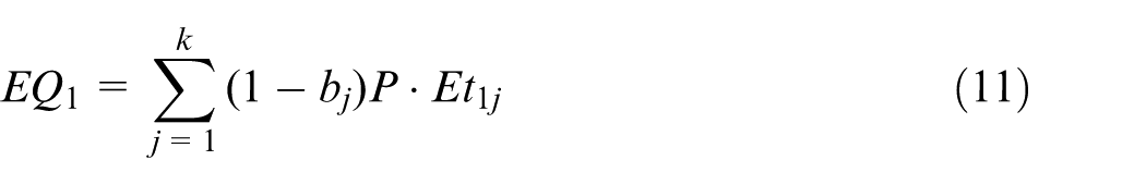
where
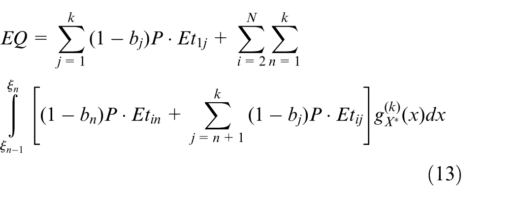
Substituting equations (11) and (12′) into equation (10), we can obtain the expression of EQ as follows
Expected total cost incurred in a renewal cycle
The total cost
The expected total PM cost incurred in a renewal cycle can be formulated as follows
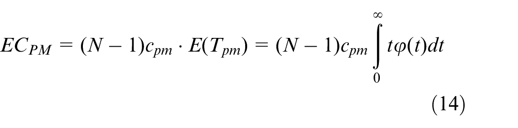
where
The replacement cost incurred in a renewal cycle is as follows

Denoting by
where
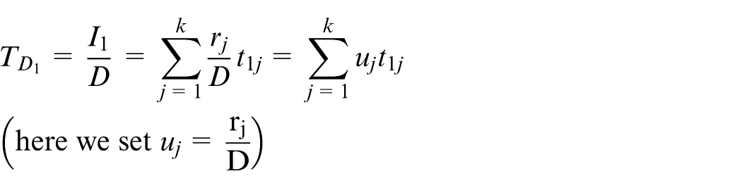
Let
According to Figure 1, the area
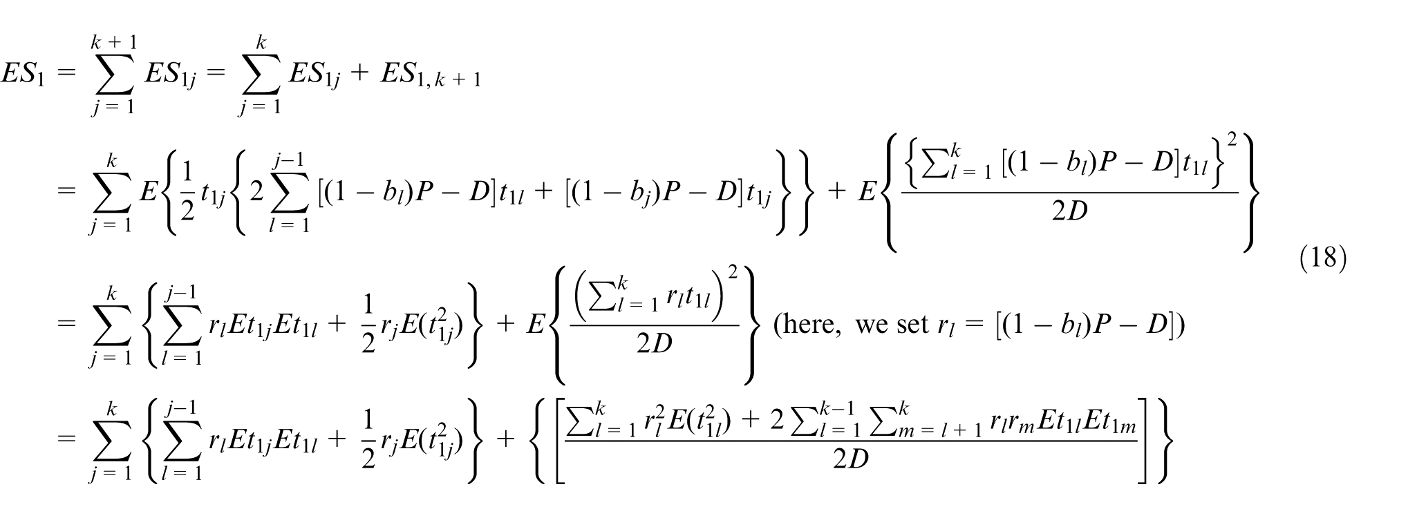
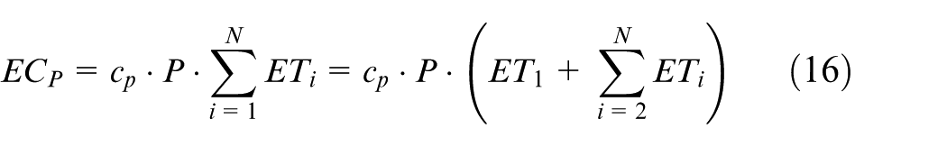
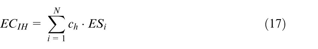
For
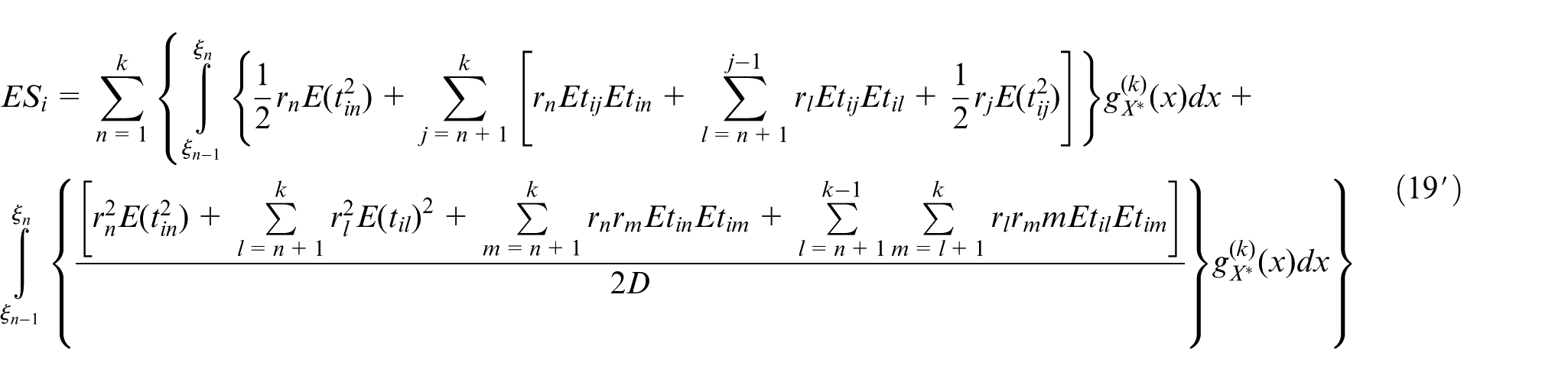
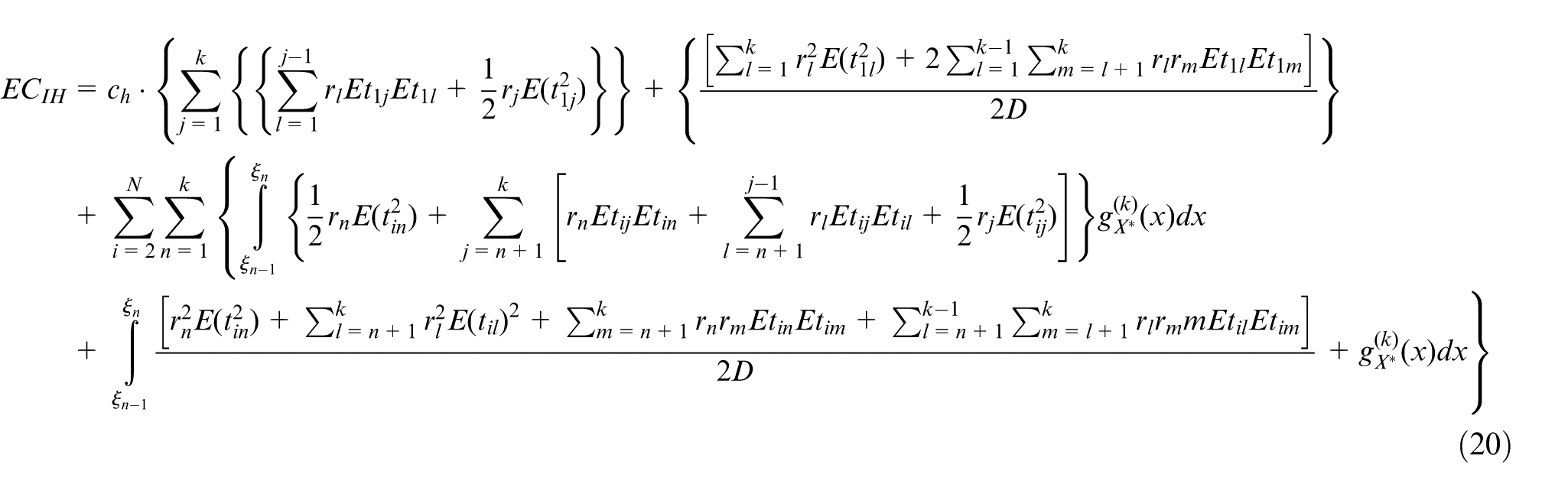
In the above calculations, we rewrite expression (19) as (19′) based on the similar consideration in the derivation of equation (12′). Substituting equations (18) and (19′) into equation (17), we can obtain the expression of
Next, we will derive the expression of the expected total penalty cost of lost sales
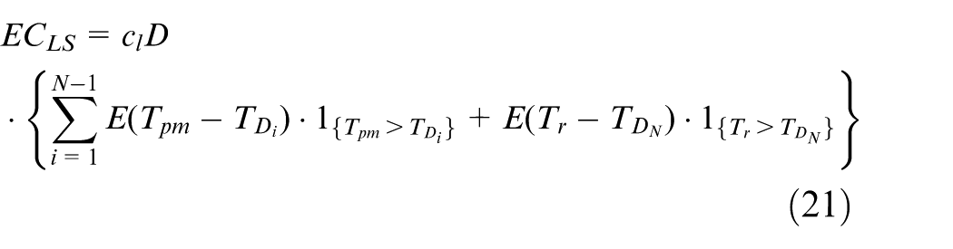
where
Consequently
It can be seen that
where
When
Consequently, we can derive the expression of
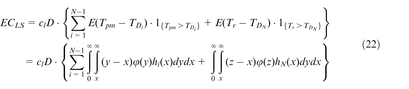
where
Now, the objective function
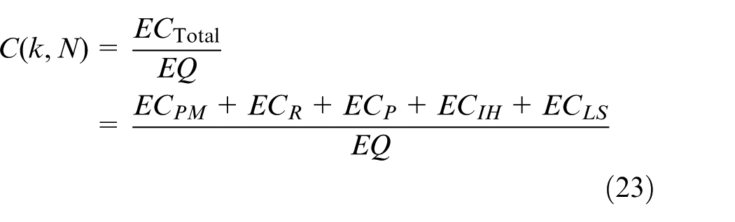
where
The objective is to determine the optimal bivariate policy
An illustrative example and discussions
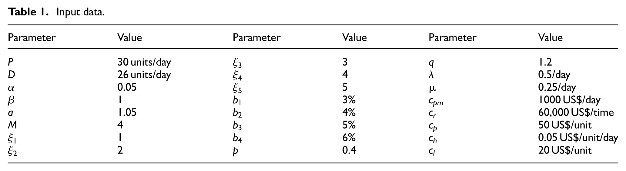
In this section, we provide some numerical results and sensitivity analysis to illustrate the model proposed. It is assumed that the distribution functions of the PM time
Input data.
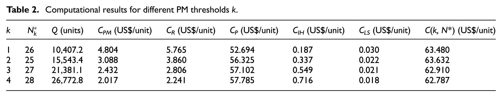
Using the computational software Mathematica 9.0, we can obtain the results presented in Table 2. For different PM threshold k (i.e.
Computational results for different PM thresholds k.
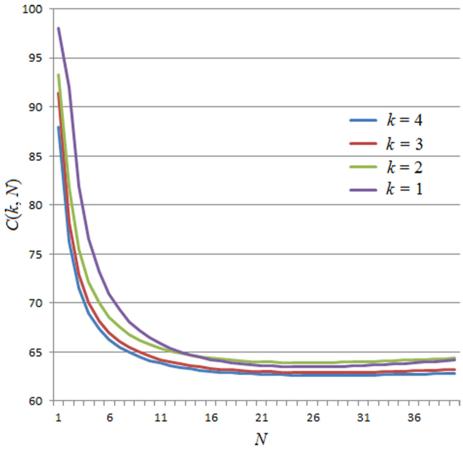
The average cost rate as function of N for different k.
It can be seen from Table 2 that the expected total quantity of conforming items produced Q increases with the increasing in PM threshold k. The PM, replacement and lost sales costs per conforming unit produced decrease as PM threshold increases. These can be explained by the fact that as PM threshold is increased, the production system works longer before PM is performed and more conforming items are produced in a renewal cycle which results in lower PM, replacement and lost sales costs per conforming unit produced. However, both the production and inventory holding costs per conforming unit produced increase as PM threshold increases. The former is due to the fact that as PM threshold is increased, the condition of the system becomes worse and worse. According to assumption A3, that is, the system produces non-conforming items at a higher rate as the degradation level increases; hence, more non-conforming items are produced and the proportion of defectives is increased which leads to a higher production cost per conforming unit produced. It can be interpreted that as PM threshold is increased, more items are produced and put into inventory. Therefore, the inventory holding cost per conforming unit produced is increased.
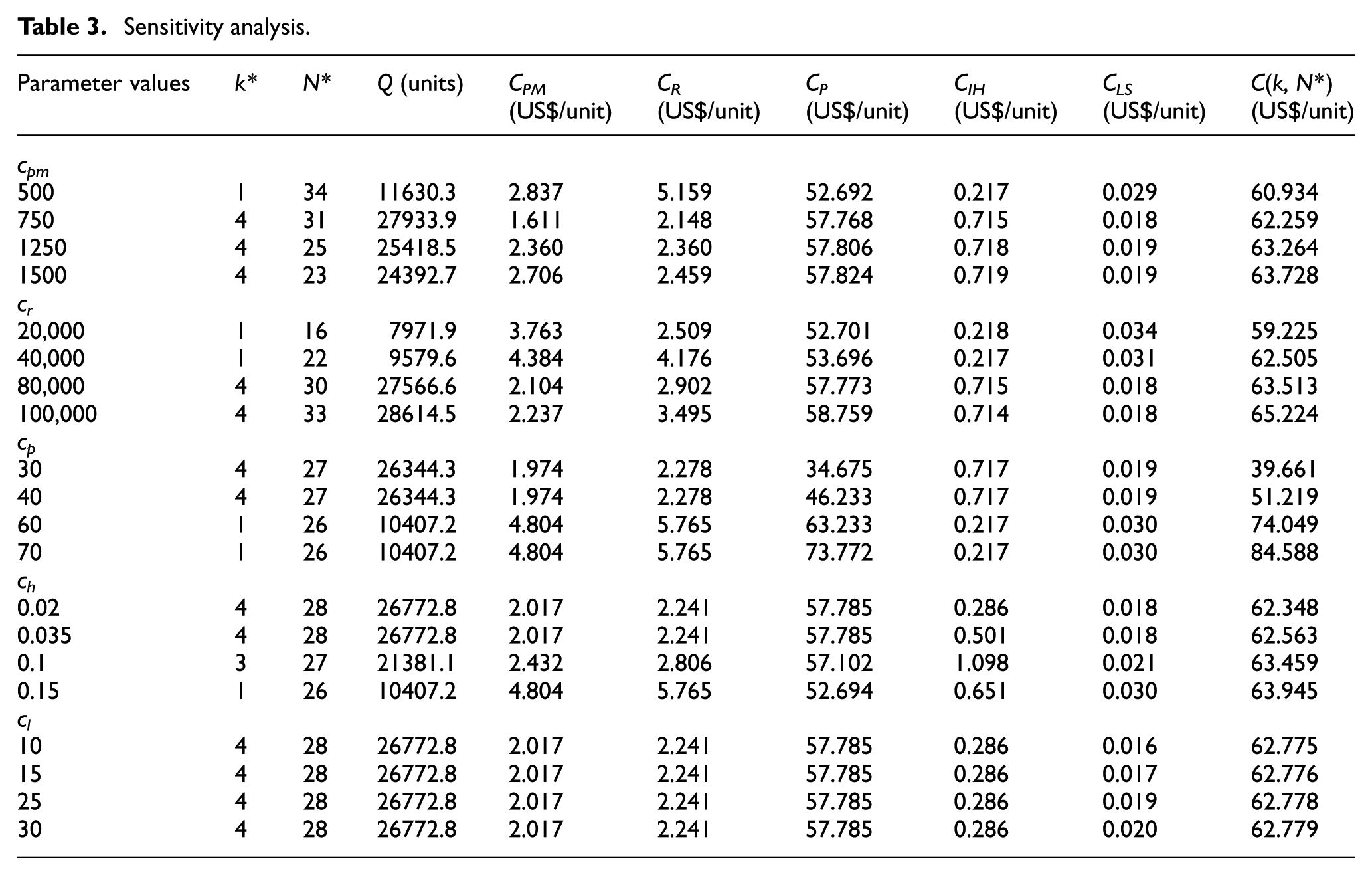
The sensitivity analysis is performed to investigate the influence of some model parameters on optimal bivariate policy as well as the expected cost rate per unit product. To this end, we vary one of the parameters at a time and keep other parameters unchanged. The results are reported in Table 3. From Table 3, we have the following observations:
As
Due to higher replacement cost
When the production cost per unit
A higher inventory holding cost per unit item per unit time
Finally, the optimal PM threshold and replacement policy are insensitive to the lost sales cost per unit item per unit time
Sensitivity analysis.
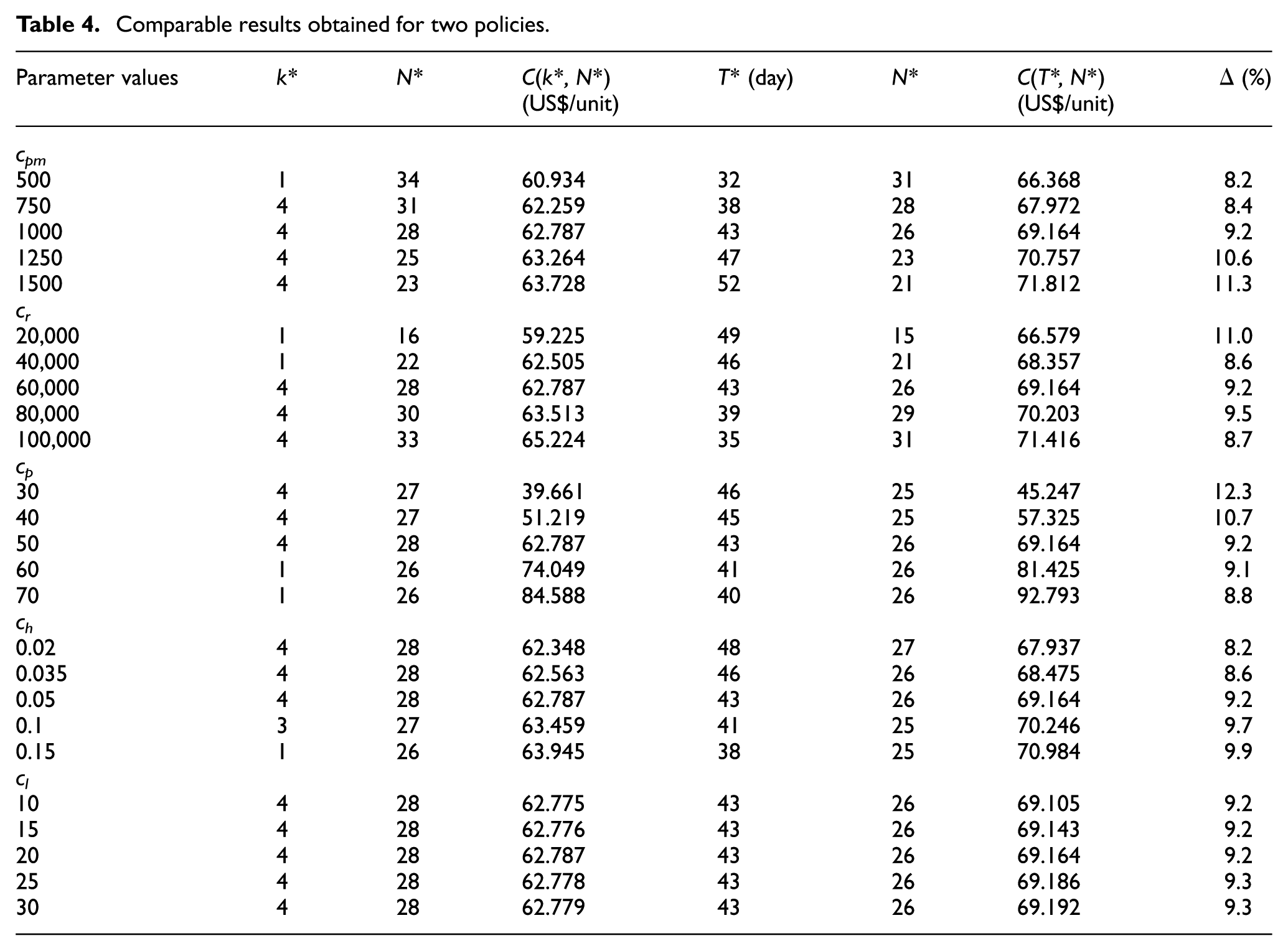
To evaluate the cost saving potential of the proposed model, we compare our results with the results obtained from the ABM model. In the ABM model, the PM is performed on production system after every T production time. Since the PM is imperfect, the system will be replaced by a new identical one after N PMs or at the system’s failure whichever occurs first. T and N are two decision variables of the ABM model. The detailed descriptions and model formulations are given in Appendix 1.
For the policy
For comparing the performance of the two policies: CBM policy and ABM policy, we compute the relative cost savings as follows
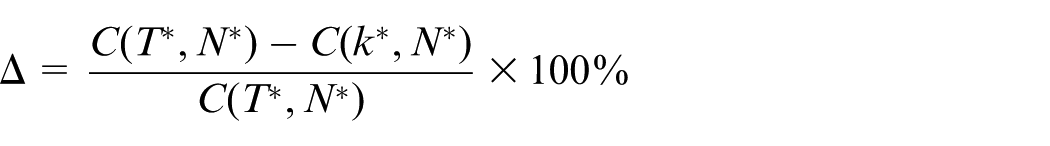
More comparable results of the two models are given in Table 4. For the 25 instances in numerical experiment, the average cost saving of CBM model is 9.4%. As expected, the CBM is more efficient than ABM due to the fact that the PM is performed based on the real-time state estimation rather than fixed time interval. The Another reason of cost reduction of CBM model lies in that the product quality is dependent on the system’s deterioration level, the CBM can control the product quality well (i.e. the PM is performed once the ratio of non-conforming items produced is higher than the warning line). In addition, as we can find in Table 4, the frequency of system replacement (
Comparable results obtained for two policies.
Conclusion
This article proposes an integrated strategy for the joint optimization of CBM and replacement policy of an imperfect production-inventory system. The production system deteriorates gradually and its degradation process is modeled by a non-stationary gamma process. For more realistic, we assume in this article a degradation-level-dependent product quality which implies that the proportion of non-conforming items being produced increases as the system deteriorates worse. To decrease the quality loss, PM is performed when the degradation level reaches the threshold, but it cannot restore the system as good as new. Hence, the aging system will be replaced by an identical new one after the Nth PM. We derived the explicit expression of the total cost per unit item
As a future work, we can relax some assumptions. A straightforward relaxation consists to consider recoverable items and rework process. This relaxation allows to deal with the scheduling problem of rework process, that is, whether the non-conforming items are reworked in the same cycle or after M cycles. Other future works can consider the random demand rate in the same context which makes the model be more realistic.
Footnotes
Appendix 1
Declaration of conflicting interests
The author(s) declared no potential conflicts of interest with respect to the research, authorship and/or publication of this article.
Funding
The author(s) disclosed receipt of the following financial support for the research, authorship, and/or publication of this article: This work was supported by National Natural Science Foundation of China under Grant Nos 61273035, 71471135 and 71661016.