
Abstract
A coupled Two-Dimension Convolutional Neural Network-Gated Recurrent Unit (2DCNN-GRU) model is proposed to evaluate and predict the hunting instability of high-speed railway vehicles in this paper. First, vibration accelerations of four measuring points on the surface of the bogie frame of a high-speed railway vehicle in good working condition and with hunting instability are obtained through a line test and model simulation. The vibration acceleration data under different conditions is cut into many pieces at equal intervals. Low-frequency band-pass filtering is applied to each piece to obtain filtered vibration data, which is then analyzed separately to get a sample set of spectrum images, including short-time Fourier spectrum, Hilbert time-frequency-amplitude spectrum, and marginal spectrum. Then, a 2DCNN model is proposed to extract features by deeply studying the spectrum images of each piece of the filtered vibration data. The root-mean-square (RMS) of the vibration responses of four measuring points on the surface of the bogie frame and the mean value of the filtered vibration response envelope are calculated and recorded for each piece. The Hunting Instability Index (HII) is proposed by considering the weighted mean of RMS and the envelope mean of the filtered vibration responses to quantitatively get the extent of hunting instability. Finally, the GRU method is applied to predicting the dynamic change of HII indicators, and the effectiveness and accuracy of the method are verified by typical examples. One contribution of this work is proposing a method to evaluate the hunting motion by image identification of the short-time Fourier spectrum, Hilbert time-frequency-amplitude spectrum, and marginal spectrum of vibration signals, and another is the definition of HII based on 2DCNN and statistics.
Keywords
Introduction
The hunting motion of railway vehicles is a self-excited vibration phenomenon first identified by Dendy Marshall 1 in the UK. Once the vibration is out of control, the railway vehicle will become unstable, and the vibration responses no longer converge, for example, periodic continuous vibration. During long-term running, the structural parameters of the rail vehicle, suspension parameters, wheel and rail surface shapes, and track irregularities are constantly changing, affecting hunting stability and running safety. Effectively monitoring the instability of the vehicle’s hunting motion and timely warning are therefore essential.
When high-speed rail vehicles run on lines, the absolute displacement of each component can hardly be measured, so through the limit cycle theory, 2 it is difficult to evaluate hunting motion. Since external excitation caused by track irregularity always exists, the characteristic signals of hunting motion are likely to be submerged in forced vibration response signals. Therefore, in practical engineering, alternative methods, such as checking whether the wheel-rail force or bogie acceleration exceeds its respective limit value, are commonly used to evaluate the stability of vehicle hunting motion.
There are two methods for monitoring wheel-rail force on-board. One is the direct method, such as the instrumented wheel-set technology, 3 and the other one is the indirect measurement method. Among all monitoring methods, the accuracy of instrumented technology is the highest. The basic principle of the instrumented wheel-set method is regarding the strain at any point of the wheel spoke surface as a function of the rolling angle and time to establish strain equations at different positions and solve these equations to obtain vertical force and lateral force. This method requires engineers to paste strain gages at certain angles on the wheel spoke surface and connect these strain gages with each other to form measurement bridges. Before using the instrumented wheel-set, the measuring bridges need to be calibrated on special equipment. Due to the high cost of a single instrumented wheel-set, it is impossible to monitor and evaluate all wheels of the train. Therefore, the instrumented wheel-set technology is not suitable for long-term vehicle monitoring.
The method most commonly used to detect hunting instability is measuring the lateral acceleration of the bogie by mounting accelerometers on the upper surface of the bogie frame. There are two types of accelerometers usually used for structural health monitoring, piezoelectric, and capacitive accelerometers. Piezoelectric accelerometers have good dynamic characteristics but cannot measure static physical quantities, while capacitive accelerometers are mostly used for measuring static and quasi-static characteristics. In rail vehicle testing, piezoelectric accelerometers are widely used for low-frequency vibration to high-frequency vibration of vehicles. At present, the research on piezoelectric accelerometers mainly focuses on the optimization of sensor performance and the development of piezoelectric materials. Reguieg et al. 4 extracted the variation curves of measurement accuracy of piezoelectric acceleration sensors with relative frequency for different damping ratios. He found that selecting a suitable damping ratio could effectively improve the measurement accuracy of sensors. Since the cut form of anisotropic piezoelectric crystal material changes the electrical properties of the crystal, which in turn affects the sensitivity of the sensor, Sinar 5 and Kim et al. 6 investigated methods to improve the sensitivity of the sensor from the perspective of material properties.
Based on the analysis of data obtained from sensors, scholars have proposed some approaches to identify hunting instability. Bruni et al. 7 proposed an original method of estimating modal parameters, such as natural frequencies and relevant damping, of vehicles running on actual lines according to Ibrahim and Prony’s methods. Ning et al. 8 and Ye and Ning 9 proposed a multi-sensor fusion feature recognition method for high-speed railway vehicles based on the Dempster–Shafer theory, which could identify small-amplitude hunting motion. Sun 10 and Zeng et al. 11 proposed cross-correlation indicators based on measured signals and indicators describing the periodicity of state variable series to detect anomalous hunting instability. Kritikakos 12 and Kulkarni et al. 13 proposed an on-board alarm signal acquisition method by collecting the bogie transverse acceleration and the axlebox transverse and longitudinal acceleration. They also proposed an on-board hunting assessment method according to the Monte Carlo method with three metrics, phase, and amplitude.
To date, there is no unified global standard for evaluating the hunting instability of rail vehicles. In Europe, UIC Code 515, 14 UIC Code 518, 15 BS EN 14363, 16 and TSI L84/132 17 have been published to address this issue. In 2013, US Federal Railroad Administration (FRA) 18 published a standard applicable to the safety evaluation of high-speed railway vehicles with speeds up to 220 MP/h. In 2019, the Standardization Administration of China 19 published the latest standard, GB/T 5599-2019, which gave a specification for testing, evaluating, and verifying the running performance of railway vehicles.
According to UIC Code 518, the standard deviation of the sum of guiding forces and the root-mean-square (RMS) of the lateral accelerations of the wheel-set and bogie frame should not exceed their respective limits. However, the evaluation of hunting instability is mainly achieved through data analysis of the lateral vibration of the bogie frame in practical engineering applications. Both UIC Code 518 and EN 14363 stipulate that the RMS of the lateral acceleration of the bogie frame should not exceed the specified limit
Engineering practices have shown that the detection of the hunting instability of rail vehicles is a complex systemic problem, and a single theory or criterion may not give accurate results. For different rail vehicles, the dynamic response to hunting instability differs with environmental conditions. Therefore, the detection of instability by comparison with limit values of the guiding forces or limit values of the bogie frame vibration acceleration may lead to unreasonable results.
In the last decade, with the development of artificial intelligence and deep learning technologies, 20 artificial intelligence-driven soft sensor technology has become an effective means of virtual measurement of key parameters, and deep-learning-based mechanical fault diagnosis has become a research hotspot. Jiang et al. 21 analyzed and summarized the key technologies of soft sensors and their applications in industrial process monitoring, controlling, and optimization. Gao et al. 22 developed a transverse pendulum angular velocity estimation algorithm based on soft sensors, Kalman filter estimation, and vehicle dynamics model and demonstrated that the soft measurement technique provided a feasible, accurate, and low-cost method for the measurement of vehicle state parameters. Sun and Ge 23 argued the necessity and significance of deep learning in soft sensor applications and summarized mainstream deep learning models, techniques, and frameworks/toolkits.
In recent years, with the installation of high-performance on-board online monitoring equipment, the intelligence of monitoring systems has become more and more advanced, monitored data has been accumulated, and the monitoring of railway vehicles has entered the “big data era.” Data-driven deep learning methods24,25 are ideal for processing massive data and identifying the presence of faults. Therefore, the self-learning of the monitored data can be used to identify running status, which provides a new means for evaluating railway vehicle dynamics performance.
The objective of this study is to evaluate and predict the hunting instability of high-speed railway vehicles. The main contribution of this study is proposing a method for hunting instability evaluation and prediction based on a coupled Two-Dimension Convolutional Neural Network-Gated Recurrent Unit (2DCNN-GRU) model by fusing image recognition and time series prediction deep learning neural networks. For the first time, the stability of hunting motion is evaluated by the image recognition of the short-time Fourier spectrum, Hilbert time-frequency-amplitude spectrum, and marginal spectrum of vibration signals, and the Hunting Instability Index (HII) based on the Convolutional Neural Network (CNN) and statistics is defined to quantify the degree of hunting instability.
The rest of this paper is organized as follows. The second part introduces the causes, characteristics, and existing detection and evaluation methods of hunting instability. In the third part, a data-driven method for evaluating and predicting hunting instability is introduced in detail. Firstly, the ways to obtain data samples through experiment and simulation are described. Then the definition of HII is given in the form of mathematical expression. Finally, a method for predicting HII indicators based on 2DCNN-GRU neural networks is introduced and verified through typical application examples.
Characteristics and assessment methods of hunting instability
Causes and characteristics of hunting instability
The vehicle track coupling system is a highly nonlinear self-excited vibration system, which can even generate a certain amplitude of hunting motion with only internal factors. The geometry parameters of the vehicle, the running speed, the characteristic parameters of the suspension system, the wheel tread profile, etc., have significant influence on the hunting stability. The differential equation for the vibration of a wheel-set is usually expressed as

Where
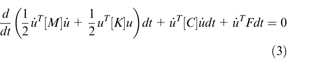
Multiplying the left side of the equation (1) by

Where
Since
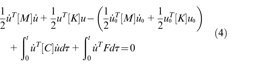
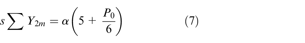
Integrating the equation from 0 to t gives
Let
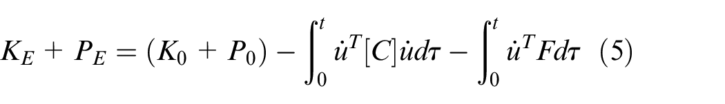
Since the dissipation function is constantly positive, the vibration energy of the system can only be provided by the wheel-rail creep force
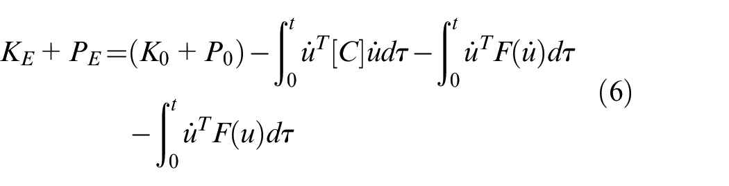
Where
The hunting motion is an inherent property of the vehicle system, and its stability must be considered in vehicle design. According to the theory of railway vehicle dynamics, the basic characteristics of hunting instability are the presence of critical speed and the Hopf bifurcation phenomenon. As shown in Figure 1, two main forms of hunting Hopf bifurcation for vehicles moving on a tangent track are sub-critical bifurcation and super-critical bifurcation. The solid and dashed lines in the diagram indicate the stable equilibrium position and the unstable equilibrium position, respectively, and the equilibrium position is the horizontal axis. The vehicle speed
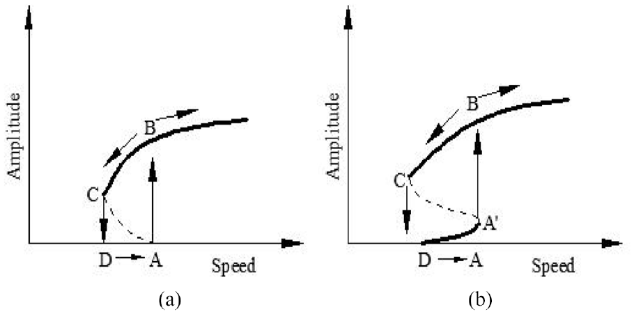
Forms of Hopf bifurcation of vehicle hunting: (a) sub-critical Hopf bifurcation and (b) super-critical Hopf bifurcation.
When the vehicle hunting instability occurs, the speed at that moment is the critical speed related to the state of track excitation. The critical speed of the vehicle running on the actual line always ranges between
Since the vibration response of the vehicle system is strongly affected by the irregular excitation of the track, the possible bifurcation forms are much more complicated than those described above. Figure 2 shows the time domain lateral displacement of the wheel-set during the acceleration and deceleration of the railway vehicle. When the railway vehicle is accelerating (Figure 2(a)), the lateral displacement of the wheel-set increases slowly with speed. When the speed of the railway vehicle reaches 264 km/h after 154 s of running, the lateral displacement of the wheel-set increases significantly, and the vehicle loses stability in its hunting motion. When the railway vehicle starts to decelerate from its maximum speed (Figure 2(b)), the lateral motion of the wheel-set obviously fluctuates due to the unstable hunting motion. When the speed of the railway vehicle drops to 255 km/h at 86 s, the amplitude of the lateral displacement of the wheel-set reduces significantly, indicating that the unstable hunting motion of the railway vehicle becomes stable.
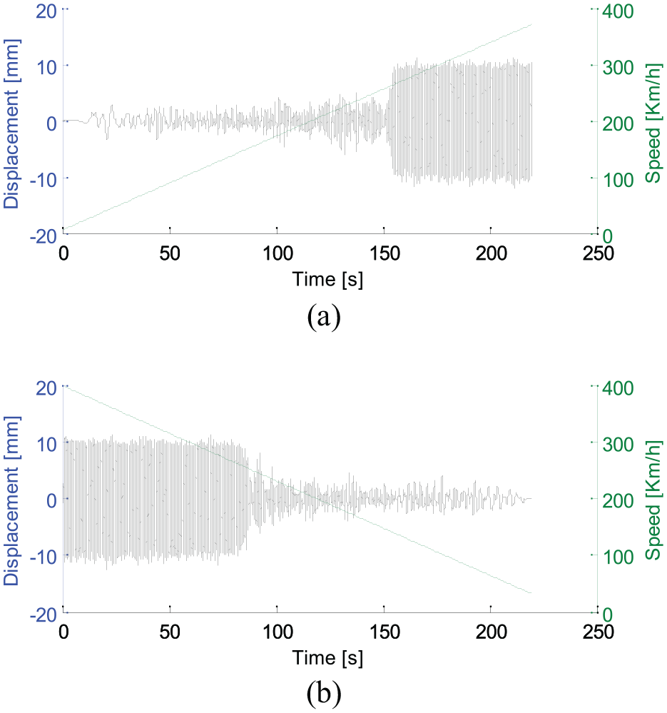
Lateral displacement of the wheel-set during acceleration and deceleration: (a) acceleration and (b) deceleration.
Figure 3 shows a typical Hopf bifurcation diagram of the lateral displacement of the wheel-set. It can be seen that the bifurcation point during deceleration is lower than that during acceleration. In Figure 4(a), the phase trajectory diagram of the lateral displacement of the wheel-set shows that the lateral displacement and lateral velocity of the wheel-set are convergent when the speed is lower than the critical speed, indicating that the wheel-set can return to the center line of the track. In Figure 4(b), when the speed exceeds the critical speed, the phase trajectory of the lateral displacement of the wheel-set leaves the initial position and forms a stable limit cycle in the phase plane.
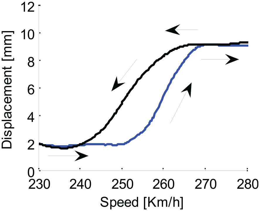
Typical bifurcation diagram for lateral displacement of the wheel-set.
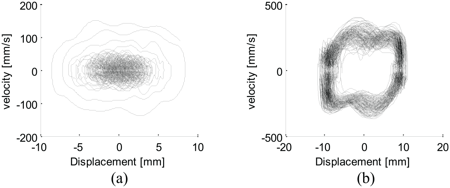
Typical phase trajectory diagram for lateral displacement of the wheel-set: (a)
Detection and assessment of hunting instability
To guarantee the running safety of trains on the line, the critical speed of the vehicle must be much greater than the maximum running speed to get enough safety margins. The critical speed obtained by the limit-cycle method mentioned above is theoretical and for reference only. In practical engineering applications, since it is impossible to check the convergence of vehicle system vibrations, the stability of the system can only be evaluated by measuring wheel-rail forces and the lateral vibration acceleration of the wheel-set or bogie frame or checking whether the continuous oscillations is attenuated.
According to the UIC code 518 published by the International Union of Railways, the guiding force of the wheel-set and the lateral acceleration of the wheel-set or bogie frame can be used to evaluate the stability of the hunting motion. First, measure the guiding force for each wheel-set and then calculate the RMS of the sum of the guiding forces for all wheel-sets (over a 100 m length in 10 m increments). The RMS limit of the sum of the guiding forces,
Where
Then, measure the lateral acceleration of the wheel-set axlebox to obtain the wheel-set lateral acceleration. The RMS calculation of the wheel-set acceleration should be carried out over a 100 m length in 10 m increments. The RMS limit of the wheel-set lateral acceleration,

Similarly, the RMS limit of the bogie frame lateral acceleration,

Where
According to the UIC code 515 published by the International Union of Railways and the standard GB/T 5599-2019 in China, the bogie acceleration is measured at the frame above the axlebox, and the assessment should cover the maximum speed. The hunting instability is identified by six or more consecutive peaks of lateral acceleration reaching or exceeding 0.8 g after filtering at 0.5–10 Hz. The criterion of hunting instability in the standard TSL L84, similar to those in UIC code 515 and GB/T 5599-2019, is that 10 or more consecutive peaks of the 3–9 Hz filtered lateral acceleration of the bogie frame reach or exceed 0.8 g.
The evaluation method based on guiding forces presupposes the on-board measurement of the dynamic wheel/rail forces, which is too costly for trains running on lines for a long time. The disadvantage of the method using the acceleration RMS of the wheel-set and bogie frame to evaluate is a large amount of calculation. Therefore, the methods specified in TSL L84, UIC 515, and GB/T 5599-2019 are more favored by engineers in practical engineering.
A new method for detecting and predicting hunting instability
Description of the proposed method
Firstly, the proposed method adopts the same measurement means as UIC code 515 and GB/T 5599-2019, including arranging sensors on the bogie frame above the axlebox and evaluating the stability of the vehicle by analyzing the collected lateral vibration acceleration. Secondly, the proposed method is data-driven, so a certain number of data samples are necessary. The data samples of the railway vehicle running on the line in good working condition can be obtained through the on-board monitoring system. However, for safety reasons, the vibration data of the railway vehicle in the case of unstable hunting is only available through rig tests or simulation models instead of line tests. Finally, the proposed method employs a 2DCNN for deeply studying the vibration acceleration spectrum to extract hunting instability features and a GRU model for predicting HII. Unlike the standards such as UIC 518, UIC code 515, TSL L84, and GB/T 5599-2019, the proposed method does not have a fixed threshold. It relies entirely on the feature identification of the spectrum of the vibration signal. In practical engineering, a library of spectrum images is required to accurately evaluate the hunting instability.
The flow of the proposed method for evaluating and predicting the vehicle hunting instability is shown in Figure 5. Firstly, a 2DCNN is built to extract features of the Hilbert spectrum, Hilbert marginal spectrum, and short-time Fourier spectrum of vibration data every second, and the stability of hunting motion is evaluated according to the recognition results. Then, the RMS of the lateral acceleration of the frame,
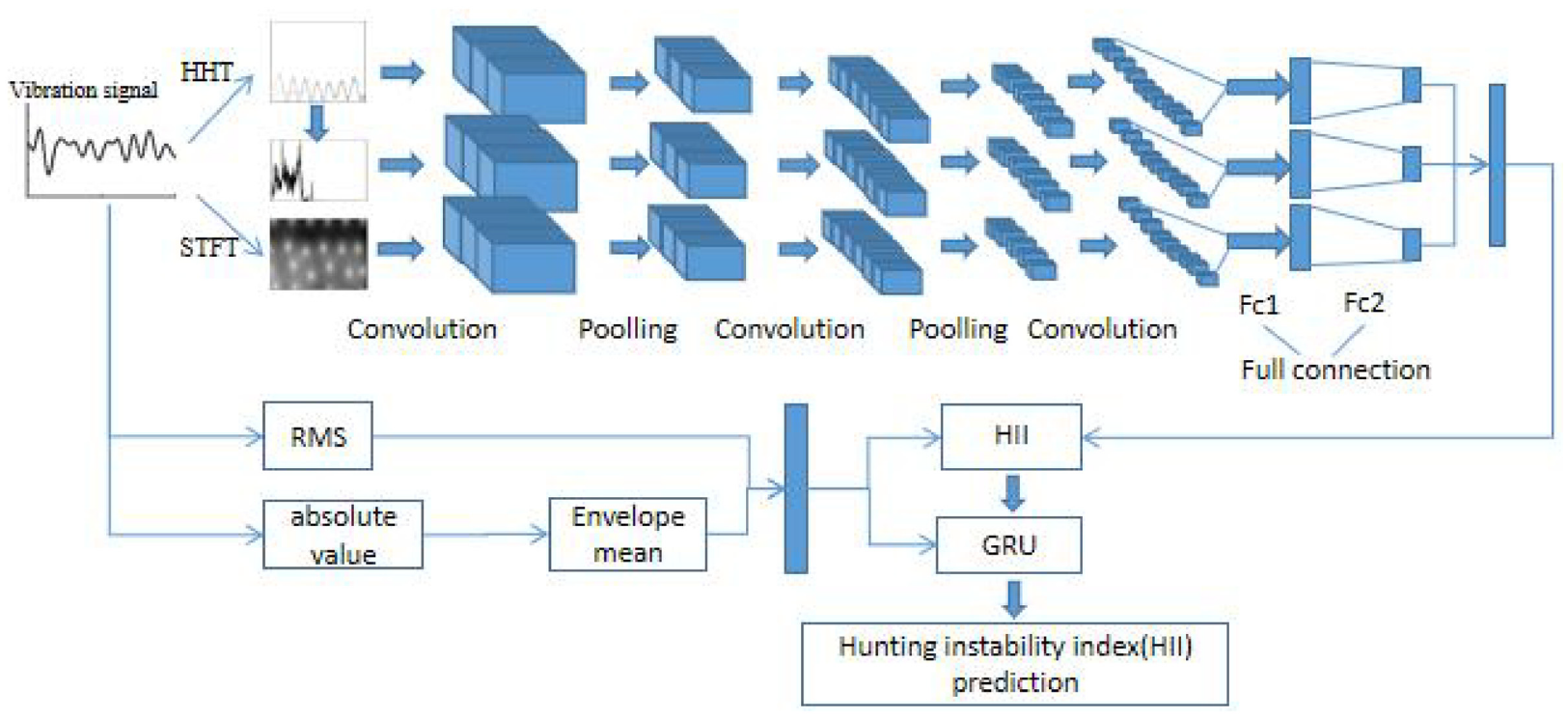
Flow of hunting instability prediction based on 2DCNN-GRU network.
The proposed method comprises the following steps:
1) Obtain the vibration acceleration samples of the bogie frame in good working condition and in the case of hunting instability. The detailed data acquisition is in Section 3.2. The time history of the vibration signal of the b-th sensor of the bogie in good working condition is expressed as
2) Cut
3) Perform short-time Fourier transform, Hilbert-Huang et al.
26
transform, and Hilbert spectrum analysis27,28 on the filtered vibration signal
4) Build a 2DCNN neural network 29 for deep learning. The designed 2DCNN neural network consists of three convolution layers, two pooling layers, and two fully connected layers. The network is applied to train the input and output data mentioned above. The calculation process is as follows.
The convolution layers in the network perform convolution calculation on the input feature images by the following formula:
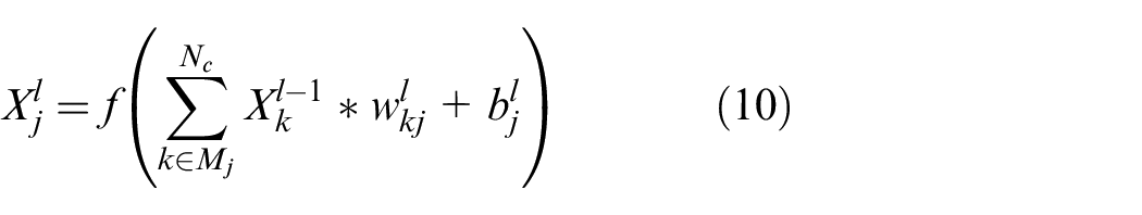
Where
The pooling layers in the network perform pooling calculation on the input feature images through the following formula:
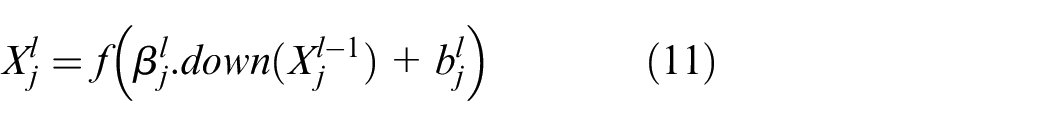
Where
The calculation formula of the fully connected layers is:

Where
5) Define HII. Calculate the RMS of
And

Where
Then HII is defined as

6) Predict HII based on the GRU 30 neural network. HII is predicted according to the following GRU neuron mathematical formula.


Where
Structure and parameters of 2DCNN network
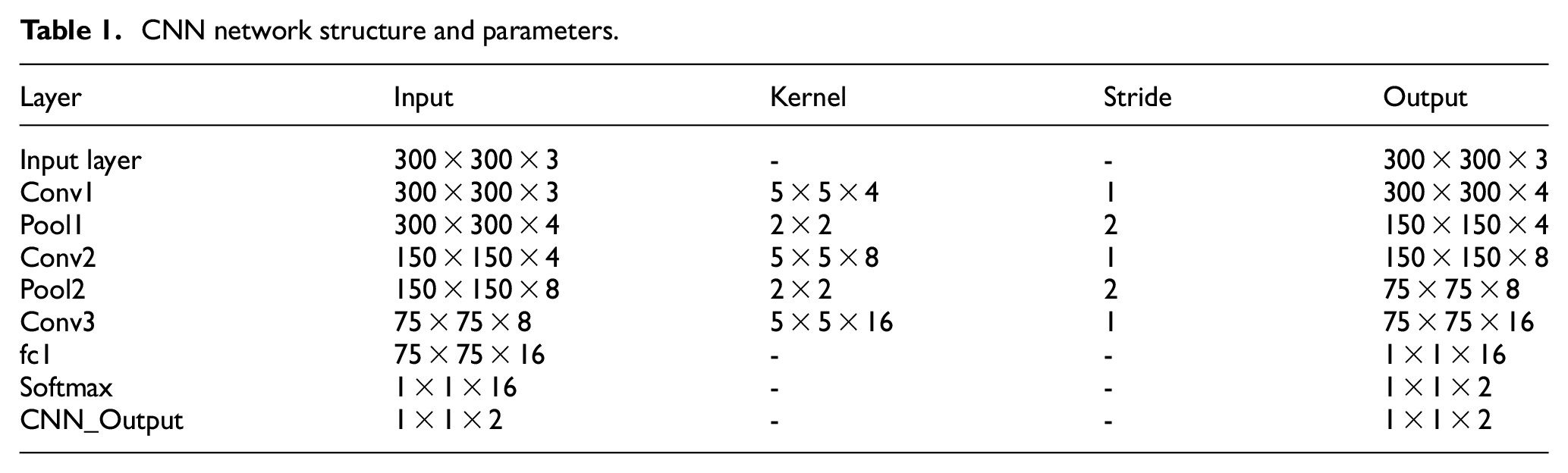
Generally, the parameters of the 2DCNN neural network designed for the first time are not optimal, so it is necessary to calculate and compare repeatedly to get the optimal parameters, which needs to consider both the accuracy of the results and the calculation time. Set the termination condition of training is that the accuracy of the 2DCNN neural network reaches 98%. The time consumption of the calculation corresponding to main parameters is shown in Figure 6. The results indicate that: (1) When the number of fully connected layers, Nfc1, is greater than 8, or the number of convolution kernels is greater than 4, the computing time is less than 30 s. (2) The time consumption increases with convolution kernel size, pooling size, pooling stride, and the number of neural network layers. (3) The optimal convolution kernel size should be less than 8 × 8, the optimal pooling size should be less than 5 × 5, the optimal pooling stride should be less than 3, and the optimal number of convolution layers should not be greater than 3. According to the above, the designed 2DCNN neural network structure is shown in Table 1, which consists of three convolution layers, two pooling layers, and two fully connected layers. The kernel size of each convolution layer is the same as 5 × 5, and the number of kernels in each layer is 4, 8, and 16. The kernel size of each pooling layer is 2 × 2, and the stride of the pooling layers is 2. The number of outputs of the fully connected layers Nfc1 is 16.
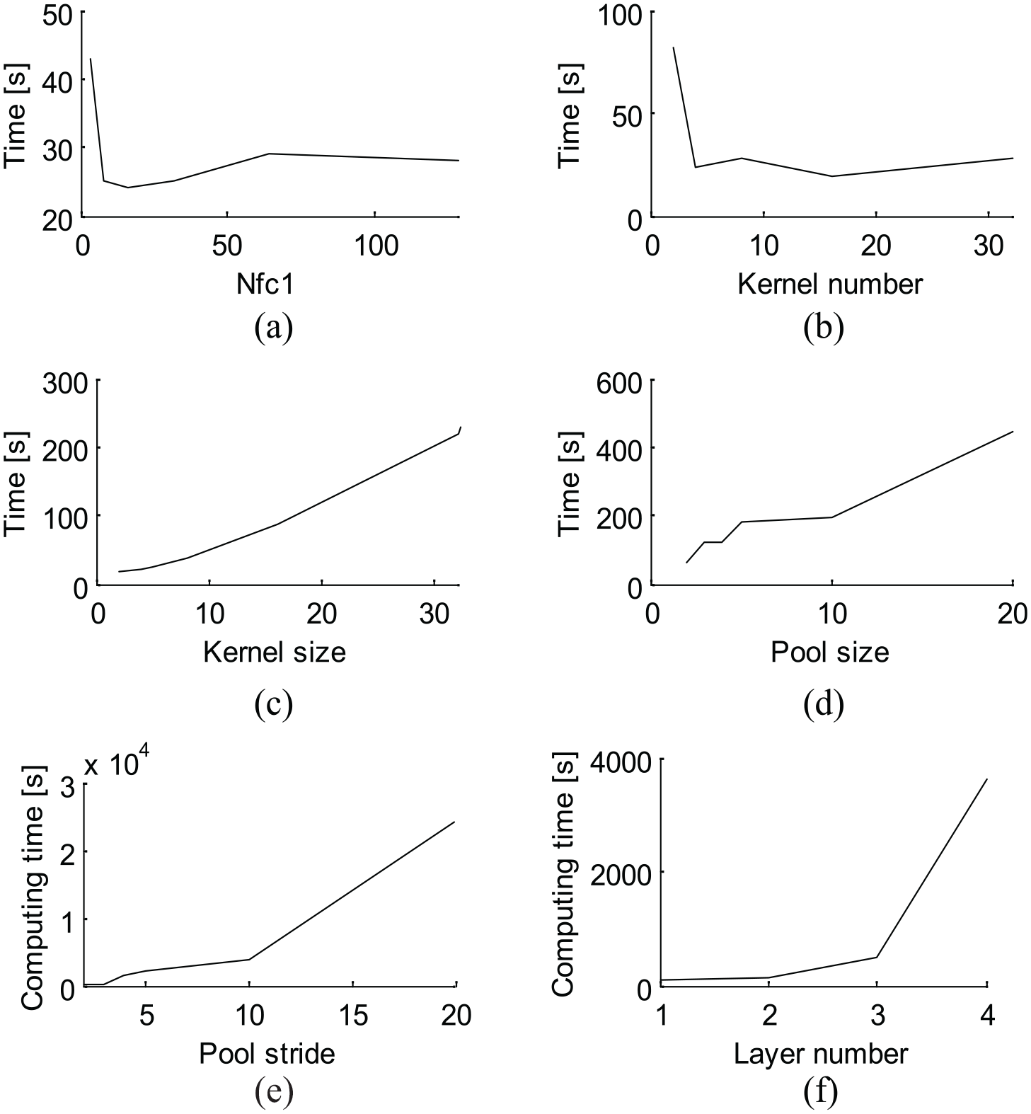
Calculation time corresponding to the 2DCNN network parameters of (a) the number of outputs of the fully connected layers Nfc1, (b) the number of kernels, (c) the convolution kernel size, (d) the pooling size,(e) the stride of the pooling layers and (f) the number of neural network layers.
CNN network structure and parameters.
Comparison of prediction networks
Deep learning models that have advantages in predicting time series mainly include the Recurrent Neural Network (RNN), 31 the LSTM, 32 and their variants, such as the Coupled LSTM, 33 the Peephole LSTM, 34 and the GRU. 30 The LSTM model is an improved model of RNN. It solves the RNN model’s inherent problems of gradient explosion and gradient disappearance, becoming an effective prediction tool for time series and nonlinear data flow. The improvement of the Coupled LSTM is combining the input gate and the forgetting gate to update the cell state. The Peephole LSTM considers the cell state in calculating the input gate, forgetting gate, and output gate, but it increases calculation costs without significantly improving the accuracy. The GRU combines LSTM’s input gate and forgetting gate into an update gate, which mixes the cell state and hidden state to generate a network structure that is almost the same as LSTM but simpler.
Based on the rig test data, this paper presents a comparative analysis of the effects of the parameters of LSTM and its two typical variants, Coupled LSTM and GRU, on prediction accuracy and time consumption. Figure 7 gives the prediction errors of three models corresponding to different learning rates. For LSTM and Coupled LSTM, when the learning rate is less than 0.001, the prediction accuracy is high. GRU has better adaptability to the learning rate and can obtain better accuracy than the other two models using the same learning rate. The prediction errors and computation time for different numbers of hidden layers are shown in Figures 8–10. For LSTM and Coupled LSTM, the errors and computation time tend to increase with the number of hidden layers. The optimal number of hidden layers for GRU is between 8 and 24, and the computation time required for achieving the same accuracy is less than the other two methods. Therefore, GRU is the most suitable network model for predicting HII.
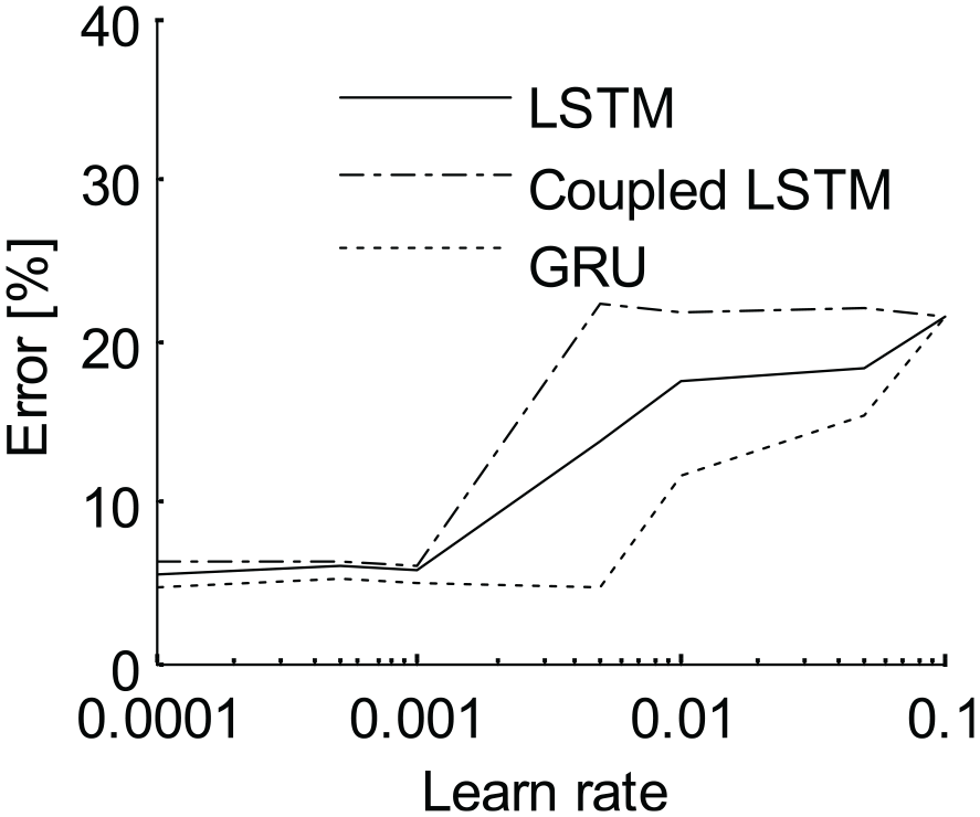
Prediction error of three methods.
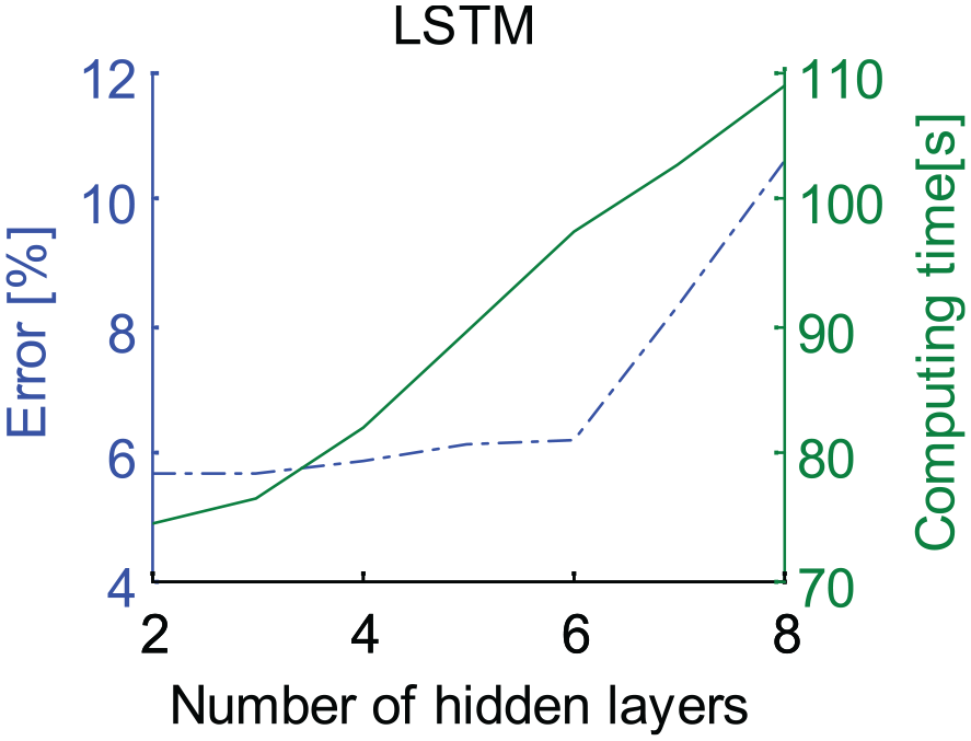
Error versus computing time of LSTM.
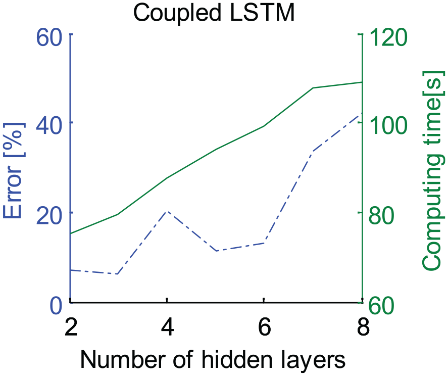
Error versus computing time of Coupled LSTM.
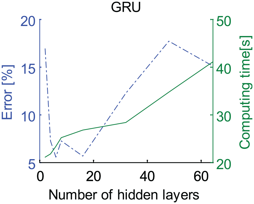
Error versus computing time of GRU.
Data acquisition of test and simulation
The data samples should include stable vibration signals of the vehicle in good working condition and abnormal vibration signals of the vehicle in a state of hunting instability. Stable vibration signals can be obtained from the on-board monitoring system. One way of obtaining abnormal vibration signals is to conduct the test on a roller test-rig, but the test speed is usually limited to a certain range due to test safety concerns. An alternative way is to build a mathematical model based on the vehicle dynamics theory or a vehicle model on a software platform to carry out simulations, so as to allow for data samples in extreme situations that cannot get from the line test or rig test.
Measurement of the bogie vibration acceleration
Before the railway vehicle runs on the line, the hunting instability test should be conducted on a roller test-rig to guarantee that the critical speed obtained in the test is far greater than the operating speed on the line, so as to have sufficient safety margins. In recent years, the on-board monitoring system for hunting instability has been mounted on high-speed trains running on lines. The sensors for monitoring hunting instability, four ZW9609A-18 accelerometers, are mounted on the bogie frame directly above the wheel-set axlebox, as shown in Figure 11. The accelerometers used are manufactured by Lance Company, with high measurement sensitivity and accuracy, ranging from −18 to 18 g, the accuracy of 0.5% FS, the lateral sensitivity ≤5%, and the frequency range of 0.5–2500 Hz. A photograph of the test site is given in Figure 12, where sensor 4 has been mounted on a bogie frame directly above the primary suspension. The sensors pass collected signals to a pre-processor, then the converted data is transmitted to an on-board host computer. The on-board host computer runs pre-programed programs to process the input signals and transmits the results to the Train Control and Management System (TCMS) network. Typically, the programs on the on-board host are written in advance according to standards UIC515, GB/T5599-2019, TSL L84, etc. Then they are embedded in the hardware system of the on-board host.
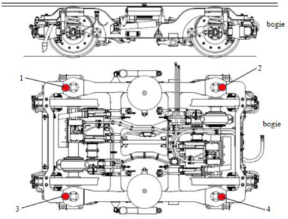
Layout of measurement positions.
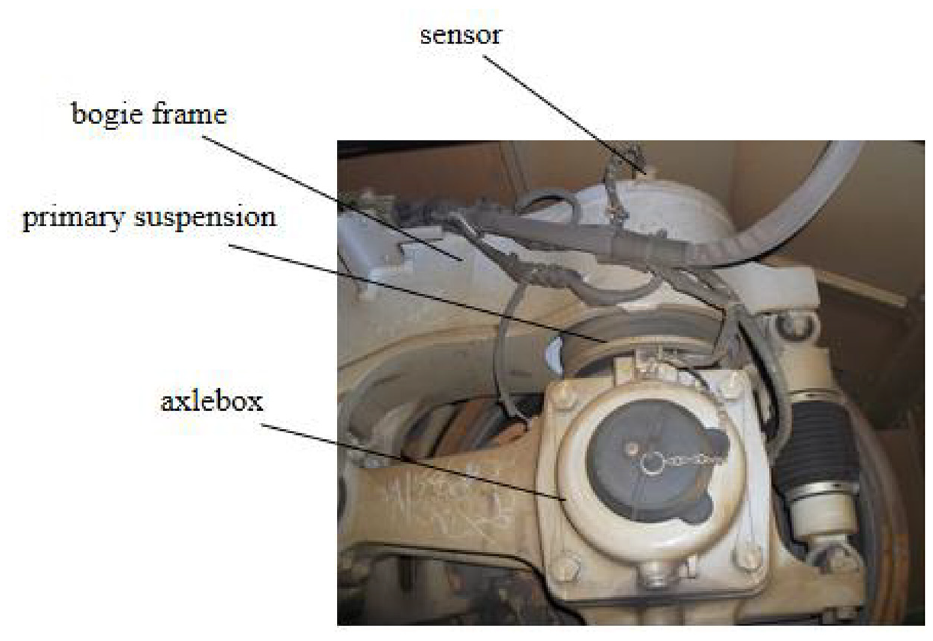
Mounting position for the sensor.
Introduction of simulation model
To objectively reflect the nature of the railway wheel-rail system, the vehicle system and the track system should be integrated into a large-scale coupling system. The wheel-rail contact model is the key node connecting the two subsystems. The coupled dynamics model used in this study consists of a sub-model of single high-speed vehicle and a sub-model of ballastless track, as shown in Figure 13. The high-speed vehicle system is composed of one carbody, two bogies, and eight wheel-sets. The bogies connect the wheel-sets and the carbody through a primary suspension system and a secondary suspension system, respectively. The wheel-sets are positioned on the bogies by the rubber nodes of the axlebox rotating arm to provide guidance and traction functions. The track system consists of rails, fasteners, track slabs, and track beds, which can effectively reduce the vibration and pressure transmitted by trains running at high speeds and ensure better track smoothness, thus helping to increase the critical speed of trains running on the line. Detailed system descriptions and equations can be found in Zhai and Wang. 35 The dynamic response of the vehicle system, such as the lateral vibration acceleration of the bogie, can be obtained by solving the model.
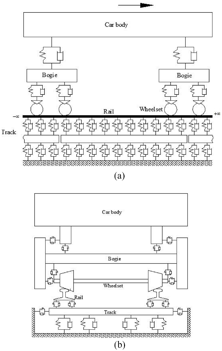
Model of vehicle-track coupled system: (a) side view and (b) front view.
Analysis of test data and simulation results
Several tests have been carried out on a rolling test-rig, with sensors 1–4 mounted on the frame. The lateral vibration acceleration of the bogie with the speed range of 80–300 km/h is obtained. For safety, the tested speed of yaw damper failure is limited to 200 km/h, and the tested speed of the vehicle in good condition is limited to 300 km/h. Figure 14 shows the RMS of the lateral vibration acceleration collected by sensor 1 corresponding to different test speeds. As the speed increases from 80 to 200 km/h, the RMS increases from 0.06 to 0.16 in good working condition and from 0.07 to 0.22 in the case of yaw damper failure. It should be noted that the hunting motion of the vehicle is stable at a speed below 200 km/h, despite the yaw dampers failure and the RMS of the vibration acceleration 25% greater than normal. In the speed range of 250–300 km/h, the RMS of the lateral vibration acceleration collected by sensor 1 increases from 0.16 to 0.34.
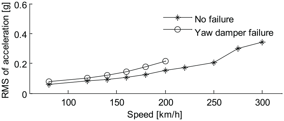
RMS of lateral acceleration of bogie frame.
After the 0.5–10 Hz band-pass filtering of lateral vibration acceleration, only low-frequency signal components within 10 Hz collected by sensor 1 are retained in the filtered data, as shown in Figure 15. The amplitudes of filtered signals corresponding to different running speeds are shown in Figure 16. When the vehicle works normally, the vibration accelerations after filtering according to the standards GB/T 5599-2019 and TSL L84 are 0.20 and 0.21 g at the speed of 300 km/h, respectively. In the case of yaw dampers failure, the maximum vibration accelerations after filtering according to the standards GB/T 5599-2019 and TSL L84 are 0.18 and 0.20 g at the speed of 200 km/h, respectively. The amplitude does not reach or exceed 0.8 g, and the hunting motion of the bogie is stable. Therefore, these standards can hardly determine whether yaw dampers work normally or detect potential instability risks.
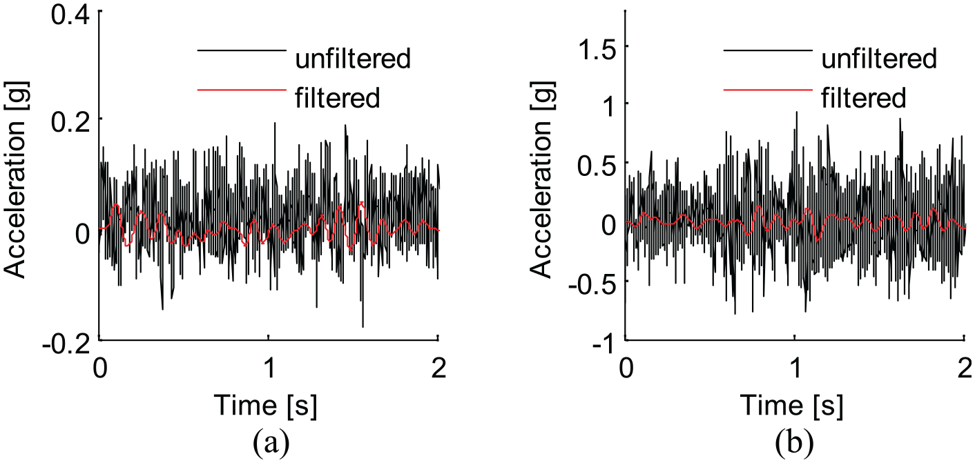
Filtered lateral acceleration of bogie frame: (a) speed = 80 km/h and (b) speed = 300 km/h.
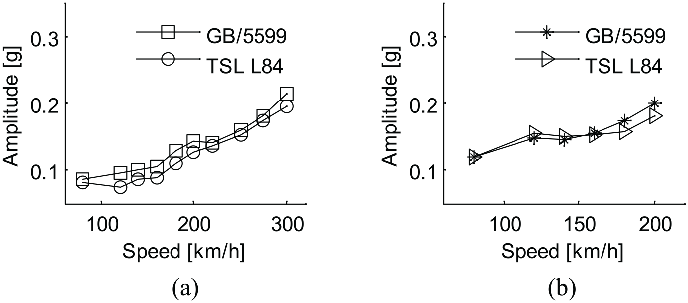
Amplitude of filtered lateral acceleration of bogie frame: (a) no failure and (b) yaw damper failure.
The line test data comes from an on-board online monitoring system, which has been mounted on a high-speed train running on the Beijing-Shanghai line for a long time. A vehicle dynamics model was developed based on the aforementioned vehicle-track coupling dynamics theory. The vibration responses of the bogie were calculated under different working conditions. The time domain responses of the filtered bogie frame vibration acceleration obtained from the line test and simulation when the vehicle was running on the straight track at a speed of 350 km/h are given in Figure 17. The simulation result is in good agreement with the line test result, indicating the great accuracy of the model, which will be used to simulate the high-speed hunting instability scenario that cannot be achieved by the line test.
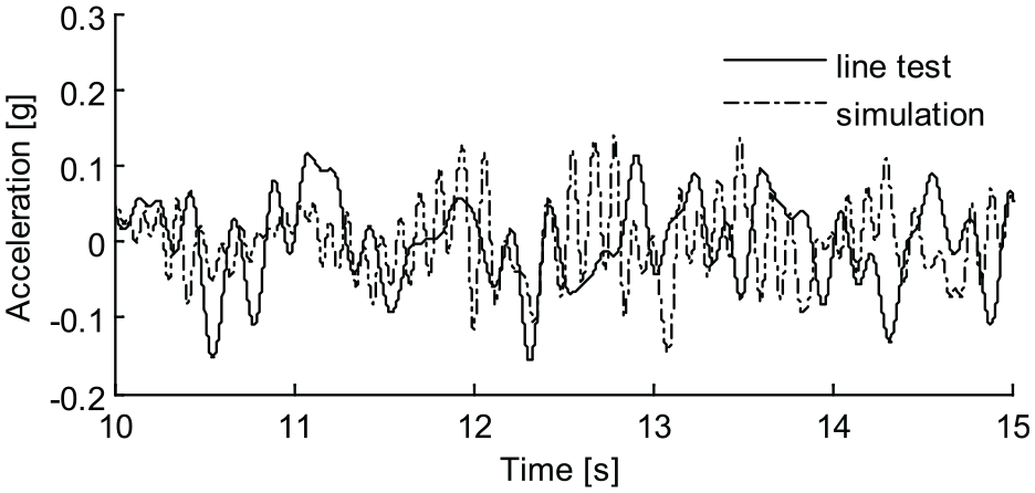
Filtered lateral acceleration of bogie frame.
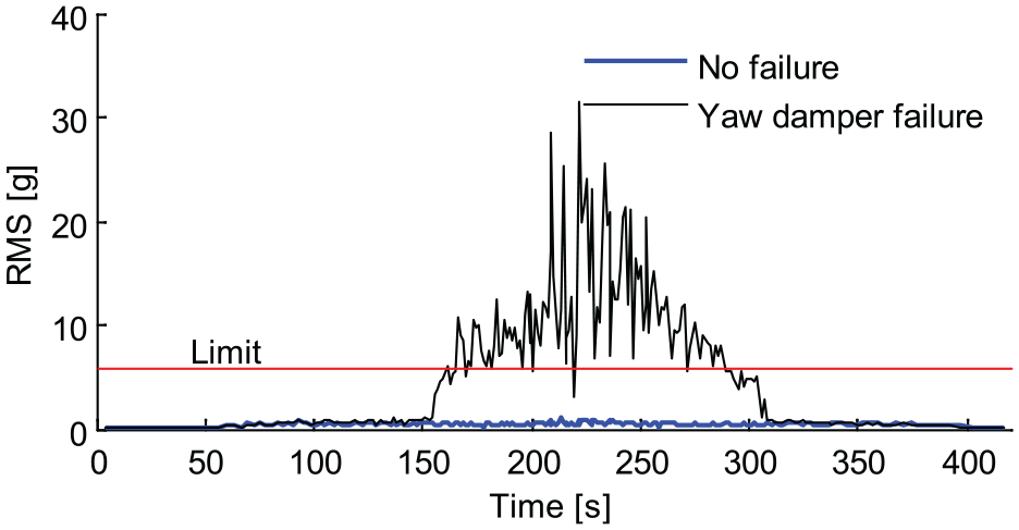
Figure 18 gives the filtered bogie lateral vibration acceleration for the whole process of the vehicle accelerating from a speed of 0 to a maximum speed of 370 km/h and then decelerating to zero. As shown in Figure 18(a), when the vehicle is in good working condition, the acceleration of the frame’s lateral vibration after band-pass filtering at 0.5–10 Hz increases with speed, and the maximum value of 0.24 g does not exceed the limit specified in the standards GB/T 5599-2019 and TSL L84, indicating that the vehicle’s hunting motion is stable. Figure 18(b) shows that when the yaw dampers fail, the lateral acceleration after 0.5–10 Hz band-pass filtering increases rapidly at t = 155 s. Figure 18(c) shows that some peaks exceed 0.8 g after 158 s, and six consecutive peaks exceed 0.8 g at 177 s. After 177 s, the vibration amplitude continues to increase with speed. When the speed achieves the maximum value of 370 km/h, the filtered lateral vibration acceleration of the frame increases to the maximum value of 2 g. While some peaks exceed 0.8 g at the time between 155 and 177 s, there are no six consecutive peaks exceeding 0.8 g, so the hunting motion of the vehicle is stable according to the standard GB/T 5599-2019. In fact, from the time of 155 s onward, the hunting motion of the vehicle becomes unstable, and the warning time obtained according to the criteria is delayed by 22 s.
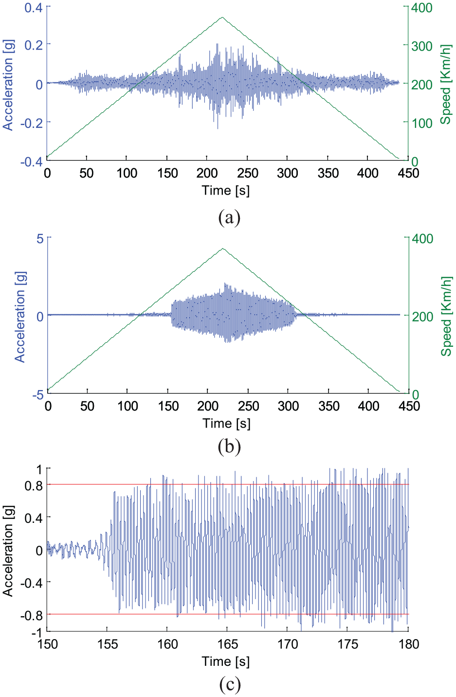
Filtered lateral acceleration of bogie frame: (a) yaw damper is normal and in good condition, (b) yaw damper is malfunctioning and the hunting motion is unstable, and (c) partial enlarged view.
Similar results can be obtained according to the standard TSL L84. The peaks exceed the limit value specified in the standard at the time of 204 s, 49 s later than the instability onset time. Figure 19 shows the curves of the moving RMS of the frame lateral acceleration versus time. In good working condition, the RMS of the frame lateral acceleration does not exceed the limit value specified in UIC 515. In the case of damper failure, the RMS of the frame lateral acceleration exceeds the limit value specified in UIC 515 at the time of 161 s, 14 s after the onset of the hunting instability. Therefore, the detection of hunting instability according to standards GB/T 5599-2019, UIC515, and TSL L84 may cause a delay in warning time.
RMS of lateral acceleration of bogie frame (over a 100 m length in 10 m increments).
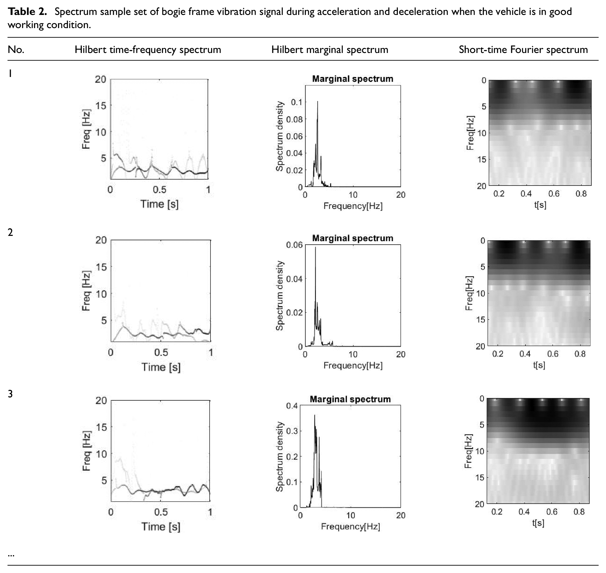
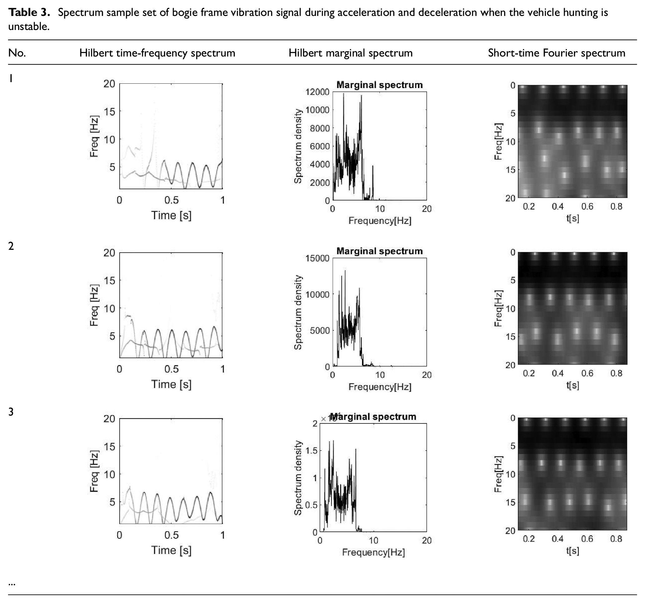
The filtered time domain signal of the frame lateral vibration acceleration is split at 1-s intervals to obtain data pieces. Each data piece is then band-pass filtered according to GB/T 5599-2019 or TSL L84. Finally, the time-frequency analysis of the filtered data is carried out to obtain the Hilbert time-frequency amplitude spectrum, the Hilbert marginal spectrum, and the short-time Fourier spectrum for each piece. The spectrum images of the data pieces corresponding to the vehicle in good working condition constitute the normal sample set, and the spectrum images of the data pieces corresponding to the hunting instability constitute the abnormal sample set. The sample set of the spectrum corresponding to the frame vibration signal in Figure 18(a) is shown in Table 2, and the sample set corresponding to the signal in Figure 18(b) is shown in Table 3. The two tables give the Hilbert time-frequency amplitude spectrum, Hilbert marginal spectrum, and short-time Fourier spectrum of each piece for the vehicle in two different conditions, respectively.
Spectrum sample set of bogie frame vibration signal during acceleration and deceleration when the vehicle is in good working condition.
Spectrum sample set of bogie frame vibration signal during acceleration and deceleration when the vehicle hunting is unstable.
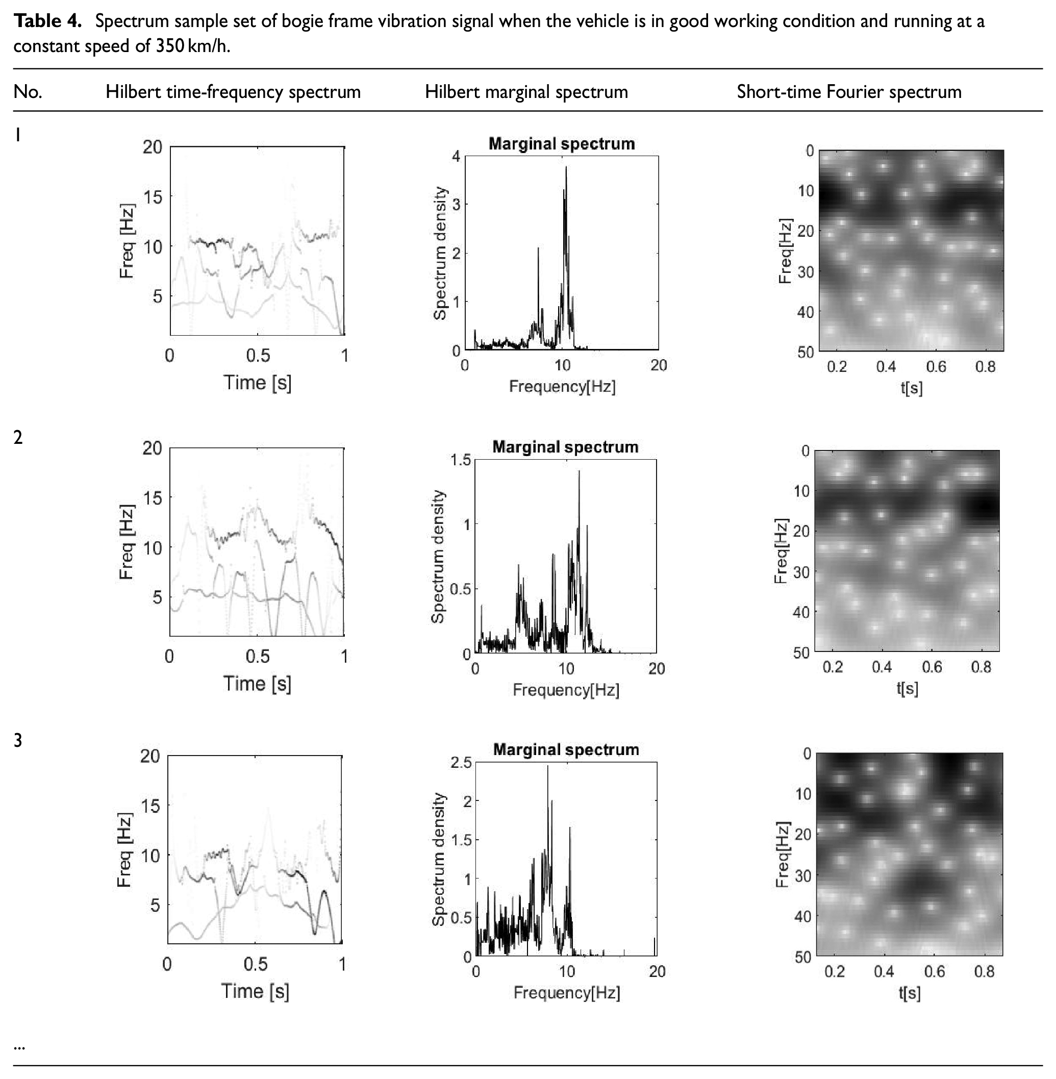
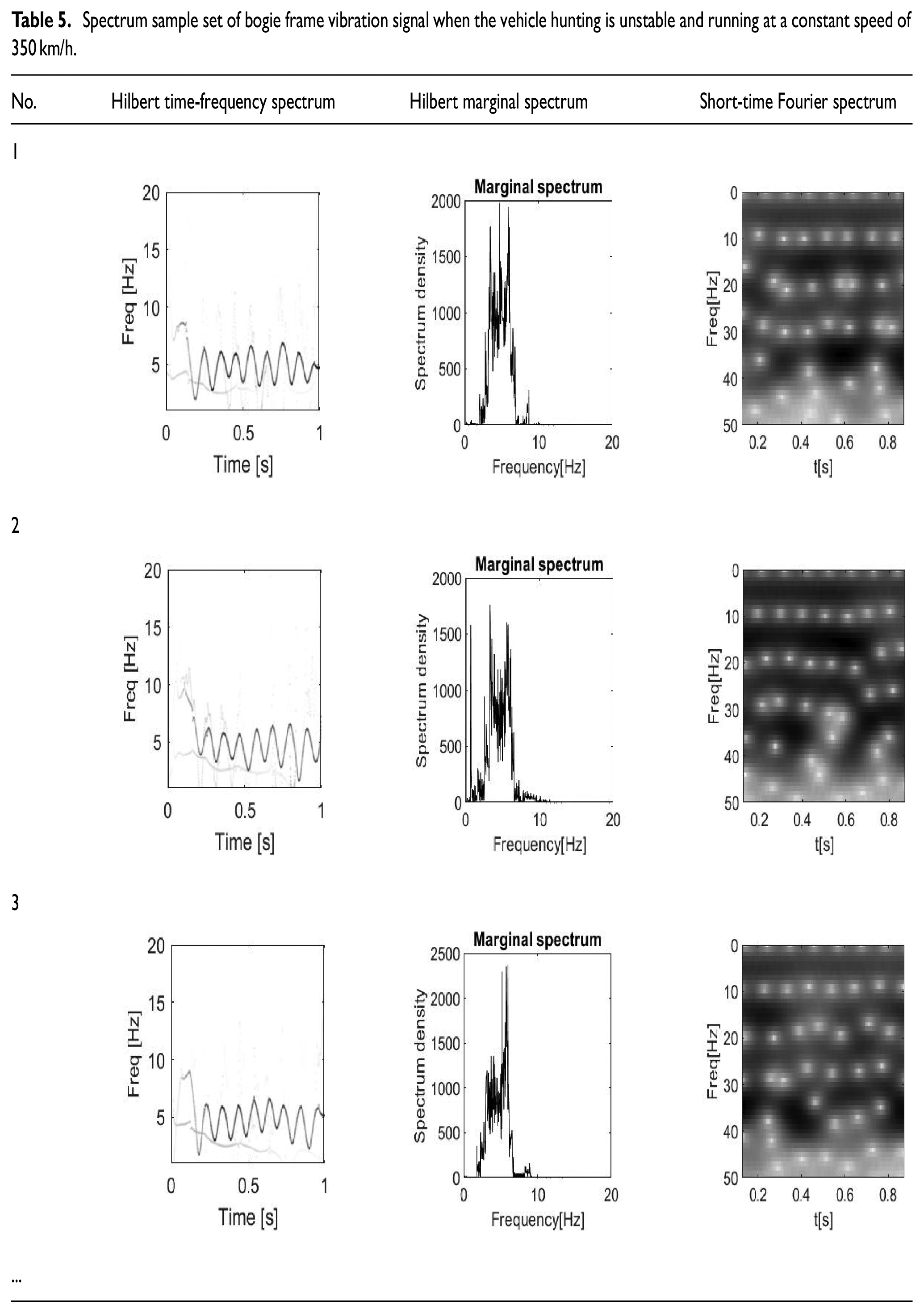
In addition to the acceleration and deceleration, the scenario of the vehicle running at a constant speed should also be considered according to the actual situation. For example, the simulation model of this study considers six different running speeds, 200, 250, 300, 330, 350, and 400 km/h. The simulation result of each running speed gives a time domain signal. The filtered time domain signal of the frame lateral vibration acceleration is split at 1-s intervals, and the Hilbert time-frequency amplitude spectrum, Hilbert marginal spectrum, and short-time Fourier spectrum at different running speeds are calculated and saved. The spectrum image samples are divided into two categories, stable and unstable. For example, samples of the filtered frame lateral vibration acceleration corresponding to the vehicle running at a constant speed of 350 km/h in these two categories are shown in Tables 4 and 5, respectively, which will be used to train and test for the 2DCNN neural network. Due to the limited space, only representative spectrum images are given in Tables 4 and 5.
Spectrum sample set of bogie frame vibration signal when the vehicle is in good working condition and running at a constant speed of 350 km/h.
Spectrum sample set of bogie frame vibration signal when the vehicle hunting is unstable and running at a constant speed of 350 km/h.
Result analysis
The following are the HII prediction results of the high-speed railway vehicle in four different scenarios. Figure 20 shows the prediction curve of HII of the vehicle during deceleration from hunting instability to stability, in which the solid line is the actual result and the dotted line is the predicted result. The results indicate that the hunting motion of the vehicle changes from unstable to stable at the time of 310 s, which is only 2 s later than the actual result (308 s). Compared the delay time obtained by calculating the RMS of bogie frame vibration acceleration described in UIC 515 with the delay time obtained by evaluating the consecutive peaks described in GB 5595-2019 and TSL l84, the predicted delay time obtained by the proposed method is significantly reduced.
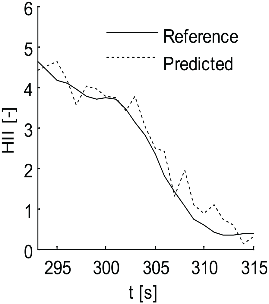
HII prediction during deceleration based on simulation results.
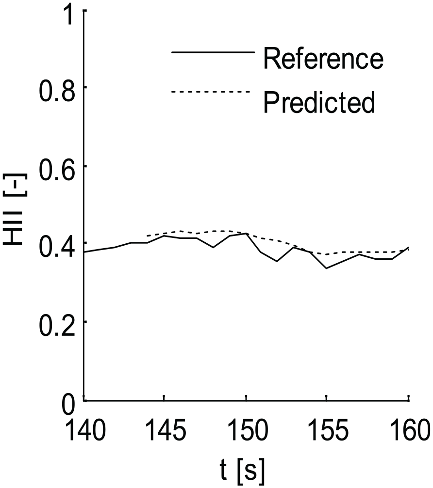
Figure 21 shows the predicted results of HII when the railway vehicle runs at a constant speed of 350 km/h on straight lines in good working condition. The predicted curve coincides with the reference curve, fluctuating in the range of 0.3–0.5, far less than 1. It indicates that the hunting motion of the vehicle is stable and has enough safety margins. Figures 22 and 23 show the predicted results of HII based on the rig test data and the line test data, respectively. When the railway vehicle is in good working condition, the predicted value almost coincides with the reference curve and fluctuates within the range of 0.4–0.6, indicating that the vehicle hunting motion is stable and has enough safety margins. The corresponding errors of the prediction in Figures 21–23 are 6.4%, 5.3%, and 9.2%, respectively, indicating that the proposed method has high accuracy in different running scenarios.
HII prediction based on simulation results at constant speed of 350 km/h.
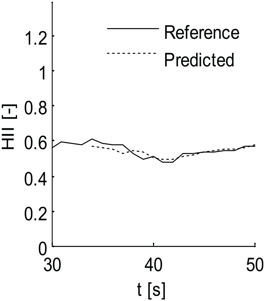
HII prediction based on rig test results at constant speed of 300 km/h.
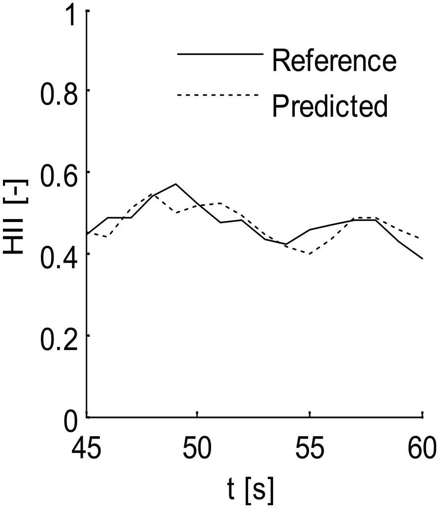
HII prediction based on line test results at constant speed of 350 km/h.
Conclusions
The methods commonly used for evaluating the hunting instability of railway vehicles are to check whether the RMS of the vibration acceleration or the consecutive peaks of the bogie lateral acceleration after filtering exceed their respective limit values. In practical engineering applications, these methods may lead to unreasonable evaluation results. This paper proposes a method for evaluating and predicting the hunting motion instability based on the 2DCNN-GRU coupling model by combing existing evaluation methods with neural network deep learning technology. Since the proposed method is data-driven, it can adapt to various situations. The 2DCNN neural network in this method identifies the features of spectrum images of hunting instability by self-learning. The defined HII is the weighted mean of the RMS and envelope mean of the filtered signal, which can quantitatively express the extent of hunting motion. The results of typical examples prove the high accuracy of the HII prediction method based on the GRU neural network. Compared with methods described in UIC 515 and GB/T 5599-2019, the proposed method can obtain more reasonable results. It provides engineers with another tool to detect and predict the hunting instability of rail vehicles.
It should be noted that the anti-hunting damper in the suspension system is the most important component in restraining the hunting motion of high-speed rail vehicles, and its dynamic performance directly affects the stability of the vehicle system. At present, the output of anti-hunting dampers of most high-speed rail vehicles is passively controlled, which cannot be adjusted reasonably according to the changes in vehicle parameters and track environment. Therefore, it is meaningful to further study actively controlling anti-hunting dampers based on this paper.
Footnotes
Declaration of conflicting interests
The author declared no potential conflicts of interest with respect to the research, authorship, and/or publication of this article.
Funding
The author received no financial support for the research, authorship, and/or publication of this article.