An effective hybrid algorithm for joint scheduling of machines and AGVs in flexible job shop

Abstract

Flexible job shops motivated by small batches and multiple orders require the collaboration of machines and automated guided vehicles (AGVs) scheduling to boost shop floor flexibility and productivity. The joint scheduling of machines and AGVs can better achieve global optimization. However, joint scheduling requires two NP hard problems to be solved simultaneously. Therefore, this paper employs a multi-AGV flexible job shop scheduling problem (MA-FJSP) with an effective hybrid algorithm. First of all, a model is established with the objectives of minimizing the makespan, the total AGV running time and the total machine load. To solve the MA-FJSP, high-quality initialization methods and improved elite strategies are designed to improve global convergence in the proposed algorithm. In addition, a problem-knowledge-based neighborhood search is integrated to improve its exploitation capability. At last, a series of comparative experimental studies were performed to exam the effectiveness of the improved algorithm. The results demonstrate that the solutions gained by the proposed algorithm perform well in respect of convergence, diversity and distribution.

Introduction

The response to diverse and individual customer needs has led to the development of multi-varieties and small-batch production model in manufacturing. ¹ The novel production pattern requires workshop to be organized according to a flexible production. To put it differently, the shop floor can designate and modify production resources in real time according to tasks to shorten delivery time. In the case of mixed production, products containing a group of operations are arranged to be processed on different machines. Likewise, each machine can be used for multi-pass machining of multiple workpieces. Although the constituent elements of jobs shop may vary, it typically includes transport resources. ² Intelligent logistics equipment like AGV is used to perform the material handling tasks, ³ which obviously improves the flexibility of the overall workshop. Therefore, considering the high correlation between AGVs and machines, research on joint scheduling of the two resources are desperately needed.

In previous research, the FJSP has been widely investigated by scholars due to its ability to reduce costs and raise yield. ⁴ To simplify the model and solve it, the transport time of the workpiece between different machines has been disregard. However, not considering transportation is not in line with realistic production, especially when the transportation of the workpiece are thoroughly dependent on the AGVs. Transport scheduling is used as a practical evaluation of the cycle time, and as important as machine scheduling, optimizing both of them will have an impact on resources and energy utilization. On the other hand, transport vehicles in the workshop are mostly non-heterogeneous AGVs and are limited in number. ⁵ Hence, the availability of AGVs brings uncertainty and complexity to current scheduling solutions.

In this paper, we consider solving two NP-hard problems simultaneously: the FJSP ⁶ and the AGV scheduling problem. ⁷ Moreover, in terms of practical requirements in the manufacturing industry, scheduling problems mostly involve multi-objective optimization. Taking into account the efficiency of the scheduling plan, three optimization objectives are considered, minimize makespan, the total AGV running time, and the total machine load. To solve this problem, the proposed approach follows two main hierarchical steps, where the elite library is used as the initial harmony memory for the harmony search (HS) algorithm. Then, in HS algorithm, a neighborhood search incorporating problem knowledge is used to guide the search in promising areas. Based on a benchmark dataset, three comparative experimental tests were carried out to test the function of the proposed algorithm.

The rest of this article is planned as follows. Section 2 presents the related research on the scheduling problem of processing equipment and transportation tools in the flexible job shop environment. In Section 3, the joint scheduling of machines and AGVs in flexible job shop is modeled as a mixed integer linear programing. Section 4 details the algorithm for solving MAFJSP. To verify the validity of the algorithm and model, a series of experimental comparative studies and discussions are presented in Section 5. Conclusions and outlook are obtained in Section 6.

Literature review

In mechanical manufacturing systems, traditional FJSP is a very complex NPhard problem. ⁶ However, in some specific production areas, transport time affects the production cycle and the quality of the product in the actual production process. Researchers considering transport time assumed that the number of vehicles is infinite, such as Zhang et al., ⁸ Dai et al., ⁹ Sun et al., ¹⁰ Karimi, ¹¹ and Huang and Yang. ¹² This assumption is clearly unrealistic. Furthermore, transport time constraints can be used for different problems, as these constraints often occur for practical problems in the industry such as: distributed job shops,^13,14 flow shops, ¹⁵ and multi-objective scheduling problems. ¹⁶ The introduction of AGVs will increase production costs, so the number of AGVs in the actual workshop is limited. The FJSP with AGV constraints is closer to the actual production situation.

Actually, Bilge and Ulusoy ¹⁷ first reported on the integrated scheduling of research machines and AGVs. Immediately afterward, a large number of researchers conducted research on the issue. Fontes and Homayouni ¹⁸ designed two sets of linked decisions to coordinate the scheduling of AGV and machine, and the authors show the effectiveness of this modeling method in finding the optimal solution.

However, few literatures consider the alternative of machines. The FJSP with AGV constraints is closer to the actual production situation. Recently, many studies have been conducted on the joint scheduling of machines and AGVs in FJSP. Deroussi and Norre ¹⁹ was the first to study this problem and proposed an iterative local search algorithm based on classical exchange, insertion, and perturbation movement. Lacomme et al. ²⁰ designed a separation graph framework for solving the FJSP problem for multiple transport robots, which can be solved for better solutions. Zhang et al. ²¹ described the job shop scheduling problem with transport constraints using a modified analytic graph and then devised an improved moving bottleneck heuristic for solving it. Nouri et al. ⁴ proposed a meta-heuristic algorithm based on an autonomous cooperative multi-agent model to solve the joint scheduling problem of mobile robots and machines. Combining the characteristics of primary and nested particles, Zhang and Li ²² designed an improved particle swarm algorithm to solve the simultaneous scheduling problem. Dang et al. ²³ studied the scheduling of mobile robots and machines in FMS and proposed a mixed integer programing (MIP) model. However, the model is only applicable to small-scale problems.

The problem of integrated scheduling of AGV and machines in FMS with conflict-free paths is investigated by Lyu et al. ²⁴ The shortest route is searched by means of a Dijkstra algorithm embedded in a genetic algorithm, and collisions of multiple vehicles are detected. The authors showed that the method is very effective in solving the benchmark problem. Fontes et al. ²⁵ considered the storage problem when addressing the collaborative scheduling of AGVs and machines. They first develop a mixed integer linear programing model and also propose a hybrid simulated annealing algorithm solution that incorporates a hill-climbing algorithm and a multi-start strategy. The computational results show the effectiveness of the model on small-scale problems. Abderrahim et al. ²⁶ proposed two local search VNS algorithms: the asynchronous VNS algorithm and the sequential LS VNS algorithm for integrated machine and AGV scheduling to minimize makespan. Comparative analysis with previous studies showed the effectiveness of the proposed model. Homayouni et al. et al. ²⁷ encoded only the process part and proposed a series of greedy heuristic rules to accomplish the machine selection task and the assignment task of the AGV. Homayouni and Fontes ² encoded three tasks, operation, machine assignment, and AGV assignment, and proposed a delayed reception hill climbing algorithm to solve them, which was tested on a publicly available data set. Chaudhry et al. ²⁸ proposed a Microsoft Excel^® spreadsheet-based solution evolver^® with a genetic algorithm program working as a plug-in to the spreadsheet environment. When seeking to solve the integrated machine and AGV scheduling problem, the paper indicates that the currently known optimal solution is found. The above paper treats the FJSP with AGV constraints as a single objective optimization problem. In contrast, multi-objective problems are widespread in practical production and require intelligent optimization algorithms ²⁹ to solve them. In recent years of research, several solution methods have emerged.

The optimization objectives of Reddy and Rao ³⁰ are makespan, the average flow time of the job and the average delay of the job, and a hybrid genetic algorithm is proposed to solve them. In the problem of machine and AGV integration scheduling, in order to obtain a scheduling solution that minimizes makespan and average drag time, Nageswararao and Rao ³¹ proposed a flock algorithm and test the effectiveness of the algorithm on benchmark cases. However, they did not present a mathematical model for this problem. Most recently, Barak et al. ³² developed a mathematical model to minimize cost and minimize integrated energy consumption. Then, they proposed an improved multi-objective particle swarm optimization to solve it. From the perspective of reducing energy consumption and cost, Liu et al. ³³ presented a green FJSP containing crane transport equipment. To solve this problem, a mixed integer programing model was first developed, then a hybrid algorithm was put forward to solve it. Similarly, He et al. ³⁴ integrated multiple AGVs into a job shop environment and proposes a multi-objective scheduling model that aims to simultaneously minimize the maximum machine time, the total idle time and the total energy consumption of the machines and AGVs. To solve this problem, an effective multi-objective evolutionary algorithm (EMOEA) is proposed. The model is validated with 75 benchmark examples and a real-world case. To solve the joint scheduling of quay cranes and speed-adjustable vehicles, Fontes and Homayouni ³⁵ develops a mixed integer linear programing model with makespan and energy consumption as objectives and proposes a bi-objective multiple group biased stochastic key genetic algorithm to solve it. The results show that an approximate true Pareto front can be obtained. These studies have enriched the methodology for solving FJSP with AGV constraints. This paper attempts to design an effective multi-objective hybrid algorithm to overcome the limitations of a single algorithm search mechanism.

Problem modeling

Problem description

In a workshop, there are n jobs J =  (J₁, J₂, …, J_n) to be processed on m machines M = (M₁, M₂, …, M_m), and w AGVs are used to handle the transport of workpieces between machines. All operations O_ij (O_ij represents the j-th process of the workpiece J _i ) are carried out on machines with a concentration of machinable machines M_ij⊆ {M₁, M₂, ···M_m} according to a defined process route. The processing time of the operation is determined by the processing machine and the sequence of workpiece operations is predetermined. After one process operation is completed, the transport of the AGV is taken into account before the next process is carried out. When a workpiece starts machining, it needs to be removed from the loading/unloading (LU) area and transported by the AGV to the machine designated to perform the first process. Once the workpiece has been delivered to the buffer zone, the AGV is ready for the next task immediately. For each of the following processes, each job is picked up by the AGV from the machine performing the previous process, waited for the job to be completed and then brought to the machine for processing. Once all operations have been processed, they are completed.

Mathematical model

In this chapter, in order to establish the mathematical model of MA-FJSP, some assumptions are first put forward:

1. At the start of production, the initial position of all AGVs and jobs is the material station;

2. AGV can only handle one job at a time;

3. AGV and machine can run stably without failure;

4. Factors such as AGV path conflicts and collisions are not considered;

5. No need for AGV resources when adjacent processes of the same workpiece are processed on the same machine;

6. A priority exists between operations of the same job;

7. After the AGV has completed the current transportation task, it can stop at the current machine. If there is a follow-up task, the AGV will directly carry out the next transportation task without returning to the storage area;

8. Makespan is the completion time of the last process.

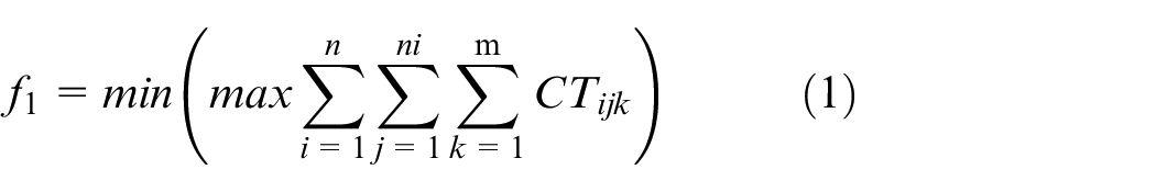
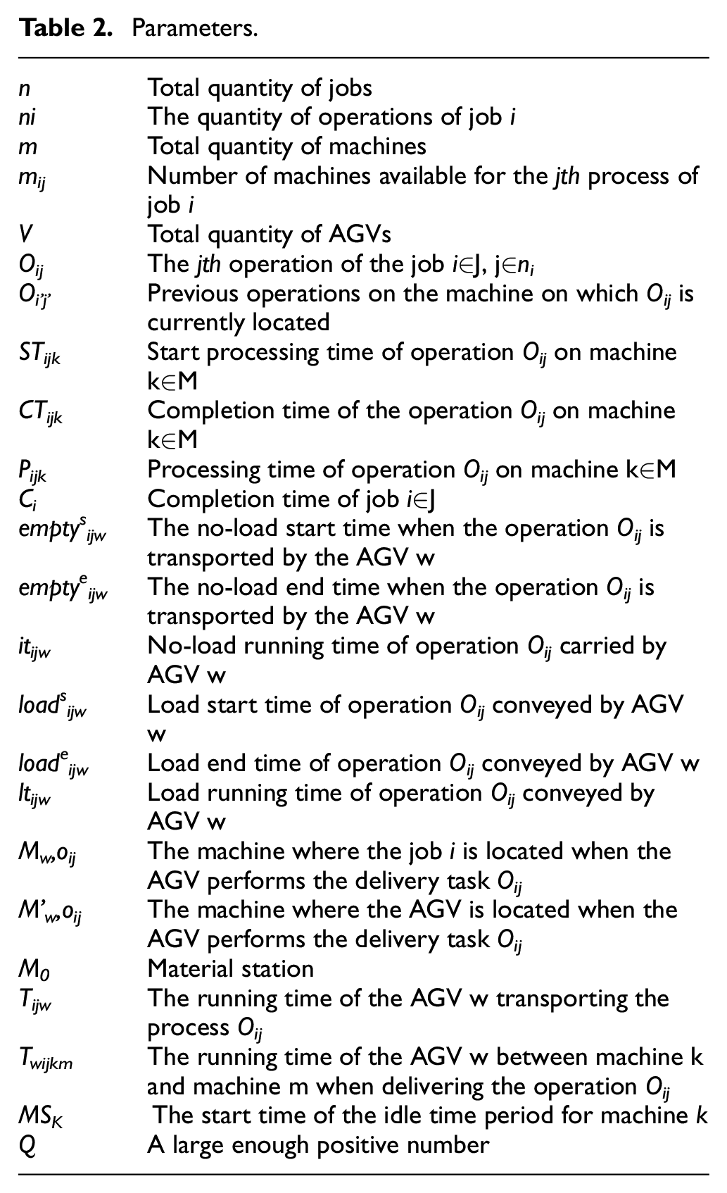
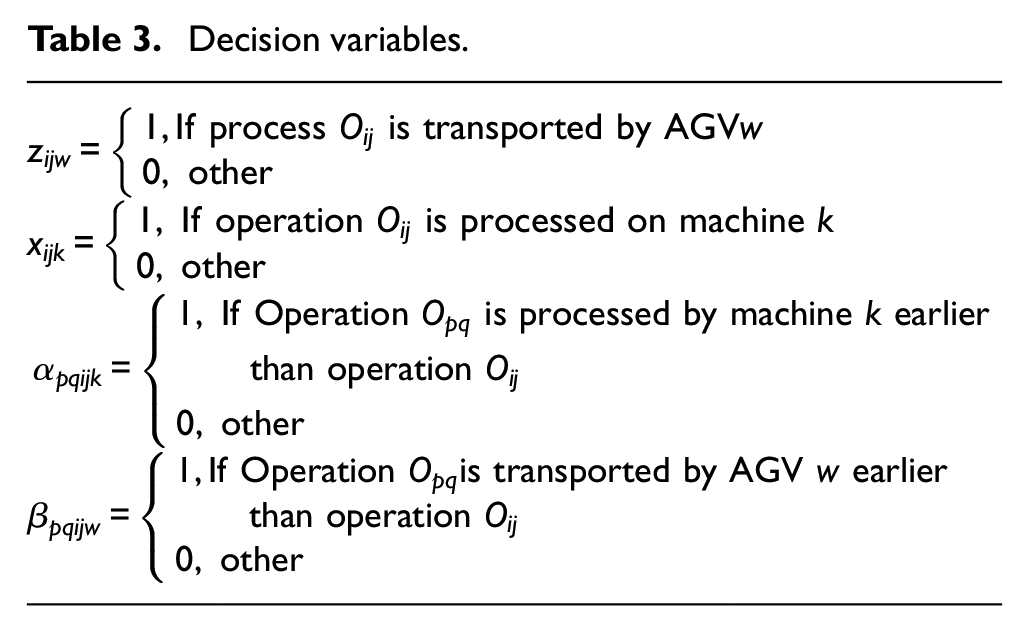
Then, to better describe mathematical models, variables, and descriptions are shown in Tables 1 to 3. Considering the production efficiency of the workshop and the loss of equipment, three objectives are considered, minimize makespan, total AGV runtime, and total processing machine load, the objective functions are given as follows:

• Object 1: Minimizing makespan means shortening the cycle time to complete orders as soon as possible.

$$f_1=\min \left(\max \sum _{i=1}^n\sum _{j=1}^{\mathrm{ni}}\sum _{k=1}^{\mathrm{m}}{\mathrm{CT}}_{\mathrm{ijk}}\right)$$

(1)

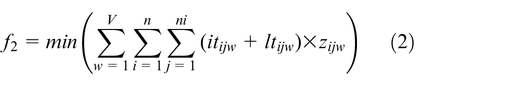
• Object 2: Reducing energy consumption of the AGV, the AGV has the shortest running distance, that is, the AGV running time is as small as possible.

$$f_2=\min (\sum _{w=1}^V\sum _{i=1}^n\sum _{j=1}^{\mathrm{ni}}({\mathrm{it}}_{\mathrm{ijw}}+{\mathrm{lt}}_{\mathrm{ijw}})\times z_{\mathrm{ijw}})$$

(2)

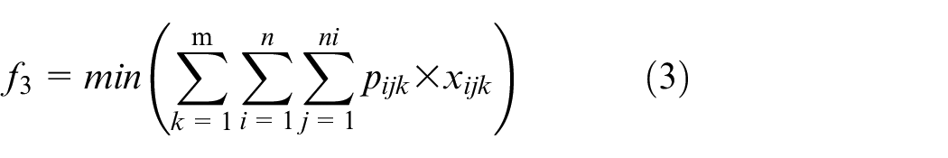
• Object 3: The decreasing total machine load means that the processing machine load is as small as possible to reduce machine energy consumption.

$$f_3=\min (\sum _{k=1}^{\mathrm{m}}\sum _{i=1}^n\sum _{j=1}^{\mathrm{ni}}{p}_{\mathrm{ijk}}\times x_{\mathrm{ijk}})$$

(3)

Table 1.

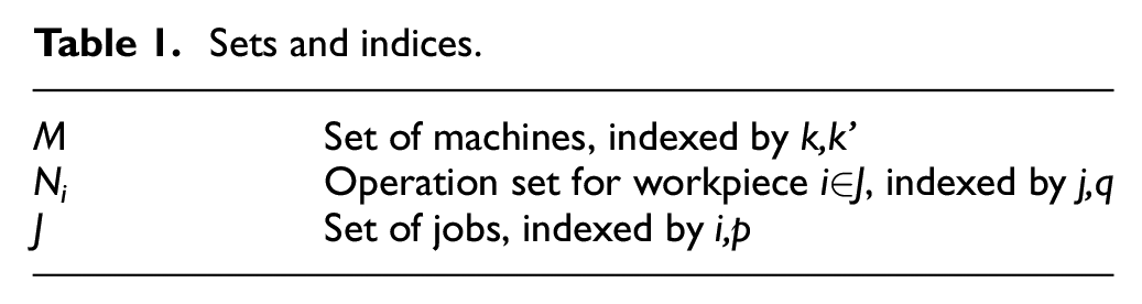
Sets and indices.

M	Set of machines, indexed by k,k’
Ni	Operation set for workpiece i∈J, indexed by j,q
J	Set of jobs, indexed by i,p

Table 2.

Parameters.

n	Total quantity of jobs
ni	The quantity of operations of job i
m	Total quantity of machines
mij	Number of machines available for the jth process of job i
V	Total quantity of AGVs
Oij	The jth operation of the job i∈J, j∈ni
Oi’j’	Previous operations on the machine on which Oij is currently located
STijk	Start processing time of operation Oij on machine k∈M
CTijk	Completion time of the operation Oij on machine k∈M
Pijk	Processing time of operation Oij on machine k∈M
Ci	Completion time of job i∈J
emptysijw	The no-load start time when the operation Oij is transported by the AGV w
emptyeijw	The no-load end time when the operation Oij is transported by the AGV w
itijw	No-load running time of operation Oij carried by AGV w
loadsijw	Load start time of operation Oij conveyed by AGV w
loadeijw	Load end time of operation Oij conveyed by AGV w
ltijw	Load running time of operation Oij conveyed by AGV w
Mw,oij	The machine where the job i is located when the AGV performs the delivery task Oij
M’w,oij	The machine where the AGV is located when the AGV performs the delivery task Oij
M0	Material station
Tijw	The running time of the AGV w transporting the process Oij
Twijkm	The running time of the AGV w between machine k and machine m when delivering the operation Oij
MSK	The start time of the idle time period for machine k
Q	A large enough positive number

Table 3.

Decision variables.

$z_{\mathrm{ijw}}=\{\begin{array}{c}1,\mathrm{If}\mathrm{process}{O}_{\mathrm{ij}}\mathrm{is}\mathrm{transported}\mathrm{by}\mathrm{AGV}w\hfill \\ \multicolumn{1}{c}{0,\mathrm{other}}\end{array}$

$x_{\mathrm{ijk}}=\{\begin{array}{c}1,\mathrm{If}\mathrm{operation}{O}_{\mathrm{ij}}\mathrm{is}\mathrm{processed}\mathrm{on}\mathrm{machine}k\hfill \\ \multicolumn{1}{c}{0,\mathrm{other}}\end{array}$

${\alpha }_{pqijk}=\{\begin{array}{c}1,\mathrm{If}\mathrm{Operation}{O}_{pq}\mathrm{is}\mathrm{processed}\mathrm{by}\mathrm{machine}k\mathrm{earlier}\mathrm{than}\mathrm{operation}{O}_{ij}\\ 0,\mathrm{other}\end{array}$

${\beta }_{\mathrm{pqijw}}=\{\begin{array}{c}1,\mathrm{If}\mathrm{Operation}{O}_{\mathrm{pq}}\mathrm{is}\mathrm{transported}\mathrm{by}\mathrm{AGV}w\mathrm{earlier}\hfill \\ \multicolumn{1}{c}{\mathrm{than}\mathrm{operation}{O}_{\mathrm{ij}}}\\ \multicolumn{1}{c}{0,\mathrm{other}}\end{array}$

The following constraints also need to be considered.

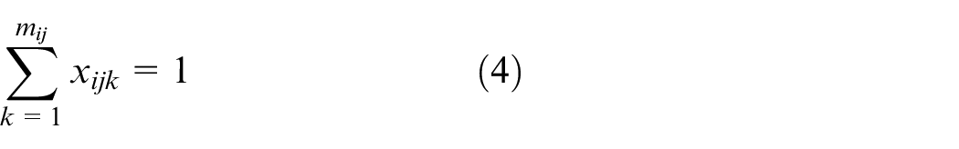
• Exclusivity constraints:

A job can only be machined by one machine at a given time work.

$$\sum _{k=1}^{m_{\mathrm{ij}}}{x}_{\mathrm{ijk}}=1$$

(4)

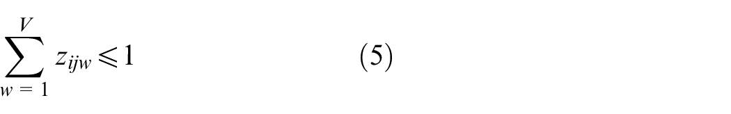
An AGV only accepts one delivery task at a time.

$$\sum _{w=1}^V{z}_{\mathrm{ijw}}\le 1$$

(5)

• Process constraints and machine resource constraints:

The start time of the job does not exceed the load end time of the AGV that undertakes the task.

$${\mathrm{ST}}_{\mathrm{ijk}}\ge \mathrm{loa}{d^e}_{\mathrm{ijw}}$$

(6)

Machining constraints of the immediate preceding process on the same machine.

$${\mathrm{ST}}_{i\prime j\prime k}+{\mathrm{CT}}_{i\prime j\prime k}\le {\mathrm{ST}}_{\mathrm{ijk}}$$

(7)

Only one process can be processed on the same machine at the same time.

$${\mathrm{ST}}_{\mathrm{ijk}}+P_{\mathrm{ijk}}\le {\mathrm{ST}}_{\mathrm{pqk}}+Q·(1-{\alpha }_{\mathrm{pqijk}})$$

(8)

• AGV resource constraints:

AGV load start time should not be earlier than the completion time of the previous process.

$$\mathrm{loa}{d^s}_{\mathrm{ijw}}\ge {\mathrm{CT}}_{i(j-1)k}$$

(9)

AGV load end time is the sum of load start time and load running time.

$$\mathrm{loa}{d^e}_{\mathrm{ijw}}=\mathrm{loa}{d^s}_{\mathrm{ijw}}+{\mathrm{lt}}_{\mathrm{ijw}}$$

(10)

AGV no-load end time is the sum of no-load start time and no-load running time.

$$\mathrm{idl}{e^e}_{\mathrm{ijw}}=\mathrm{idl}{e^s}_{\mathrm{ijw}}+{\mathrm{it}}_{\mathrm{ijw}}$$

(11)

The no-load departure time of the AGV is not earlier than the end time of the last transportation task of the AGV and the start time of the workpiece.

$$\mathrm{idl}{e^s}_{\mathrm{ijw}}\ge {\mathrm{ST}}_{\mathrm{ijk}}$$

(12)

$$\mathrm{idl}{e^s}_{\mathrm{ijw}}\ge \underset{\mathrm{pqk}}{\overset{e}{\mathrm{idle}}}·(1-{\beta }_{\mathrm{pqijw}})$$

(13)

AGV transportation time is equal to the sum of no-load time and load time.

$$l{t}_{\mathrm{ijw}}+i{t}_{\mathrm{ijw}}=T_{\mathrm{ijw}}$$

(14)

In addition, the following three factors are considered: whether the process is the first process of the job, the current position of the AGV and the working state of the machine when the job is delivered.

• The job from the material area is transferred to the designated machine to perform the first operation. The AGV working time is the sum of the transport time among the current position of the AGV, the material station, and the machine. The calculation formula is as follows:

$$T_{\mathrm{ijw}}=T_{\mathrm{wijM}0M\prime w,\mathrm{Oij}}+T_{\mathrm{wijM}\prime w,\mathrm{OijMw},\mathrm{Oij}}$$

(15)

Correspondingly, when the job is delivered, if the machine is not busy, the start time of the operation is the end time of transportation, otherwise, the start processing time of the operation is the maximum of the transportation end time and the machine starts idle time.

$$S{T}_{\mathrm{ijk}}=\{\begin{array}{c}{T}_{\mathrm{ijw}},\mathrm{the}\mathrm{machine}\mathrm{is}\mathrm{idle}\hfill \\ \multicolumn{1}{c}{\max (T_{\mathrm{ijw}},M{S}_k),\mathrm{other}}\end{array}$$

(16)

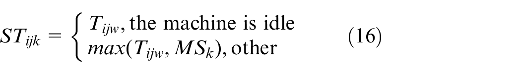
• For all subsequent operations, the job is taken by the AGV from the machine that performed the previous operation. The AGV working time is the sum of the transportation time among the current location of the AGV, the machine where the previous process is located and the processing machine. The calculation formula is as follows:

$$T_{\mathrm{ijw}}=T_{\mathrm{wijMw},\mathrm{Oij}-1M\prime w,\mathrm{Oij}}+T_{\mathrm{wijMw},\mathrm{Oij}-1\mathrm{Mw},\mathrm{Oij}}$$

(17)

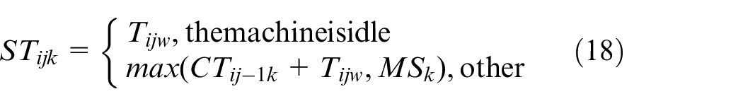
Correspondingly, if the machine is idle when the job arrives, the processing start time of the operation is equal to the transportation time; otherwise, the maximum between the sum of the completion time of the previous process and the transportation time T_ijw and the start time of the machine idle is selected as the start time.

$$S{T}_{\mathrm{ijk}}=\{\begin{array}{c}{T}_{\mathrm{ijw}},\mathrm{the}\mathrm{machine}\mathrm{is}\mathrm{idle}\hfill \\ \multicolumn{1}{c}{\max ({\mathrm{CT}}_{\mathrm{ij}-1k}+T_{\mathrm{ijw}},M{S}_k),\mathrm{other}}\end{array}$$

(18)

Proposed algorithm

The HS algorithm has been applied to scheduling problems, such as AGV scheduling problem, ³⁶ IPPS, ³⁷ and FJSP.^38,39 It has the features of simple principle, fast convergence speed and combination with other algorithms easily. In the generation of new solutions, the existing solution vectors can be fully utilized to ensure the diverseness of the population. Therefore, this paper combines the HS algorithm and NSGA-II to design a multi-objective hybrid algorithm. Figure 1 shows the flow chart of the proposed algorithm. The steps are as follows:

• Step1: Initialize population employing the strategy in section 4.3. Perform non-dominated sorting and crowding distance measure on the population P.

• Step2: Selection of individuals using tournament selection. Execute crossover and mutation to generate a new population (Q).

• Step3: Merge populations P and Q. Perform non-dominated sorting and crowding distance measure on the merged population(M).

• Step4: Perform the elite strategy in section 4.5 on M to generate a new population P.

• Step5: Initialize the harmony memory library with P and fine-tune it using two neighborhood search methods.

• Step6: Perform non-dominated sorting and crowding measure on the harmony memory library. Update the harmony memory library using the elite strategy in section 4.5 and form a new parent population P.

• Step7: If current running iteration j > harmony iterations IT2, skip to the next step, otherwise continue to execute the harmony search strategy.

• Step8: If current running iteration i > total iterations IT1, end the output of the solution in the harmony memory, otherwise continue to Step2 for the next cycle.

Figure 1.

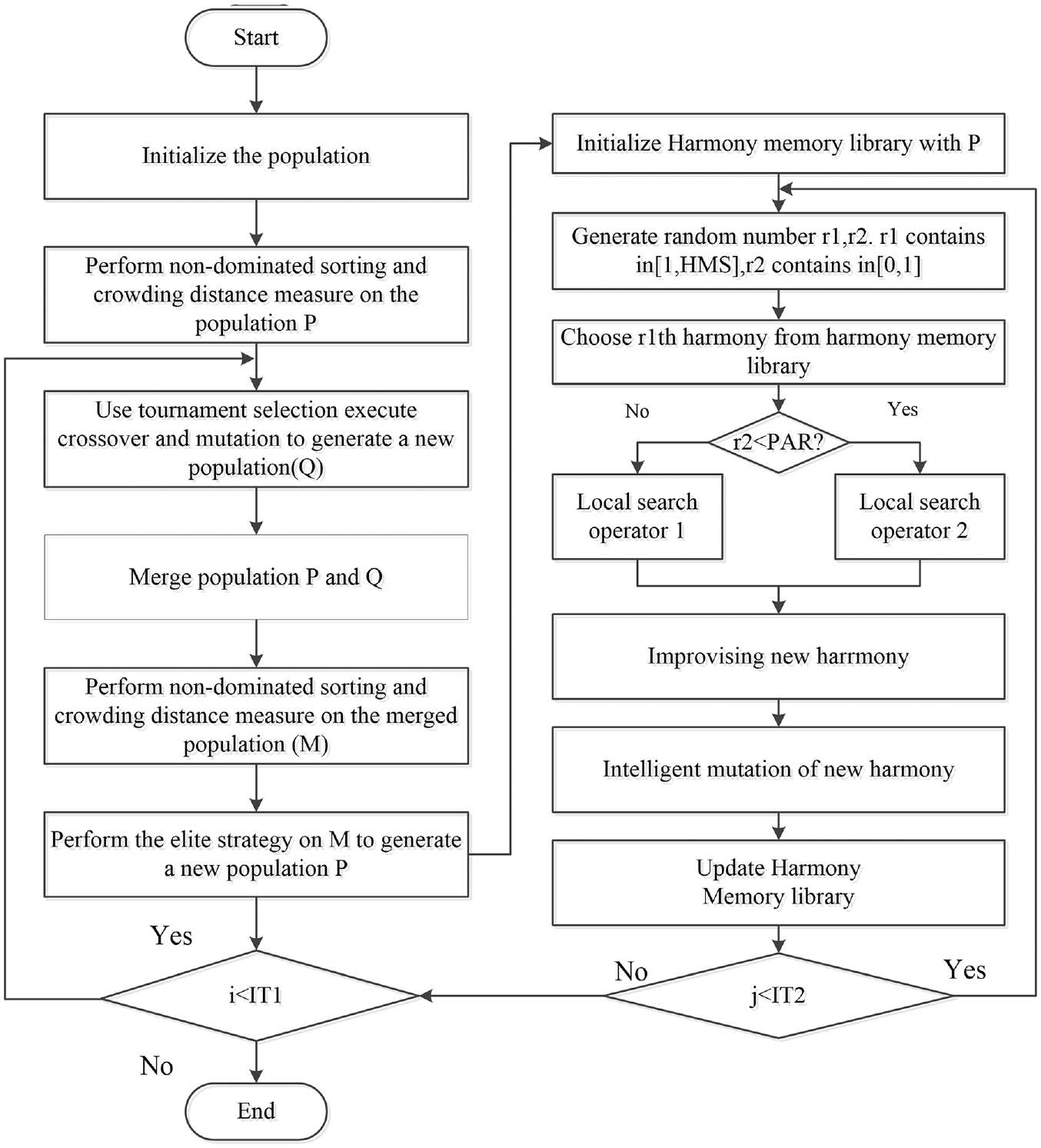
The proposed algorithm flow chart for MA-FJSP.

Encoding and decoding

When the evolutionary algorithm is used to solve, appropriate encoding and decoding strategies can improve the operating efficiency of the algorithm. This section uses an example to describe the process. The job processing information is shown in Table 4.

Table 4.

Example of 3 × 5 FJSP problem.

	Job 1			Job2			Job3
Operation	1	2	3	1	2	3	1	2
Machine	1,2,5	1,3	2,3	1,4	2,4	1,3	1,2	1,4,5
AGV	1,2

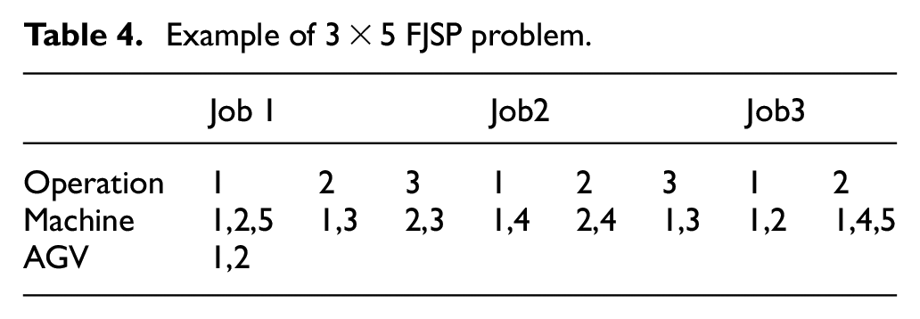
Based on the problem studied in this paper, each solution is encoded in a triplet called the operation scheduling vector, the machine selection vector, and the AGV assignment vector. Taking the process information in Table 1 as an example, there are eight operations for three jobs. The corresponding set of optional machines for each operation is some of the five machines, as well as two AGVs available. Accordingly, Figure 2 encodes the information in Table 1, and the chromosome consists of eight genes. For example, the first number 3 in the operation scheduling vector corresponds to the number 5 in the machine selection vector and the number 2 in the AGV allocation vector, which means that O31 will be transported from AGV 2 to machine 5. Using this coding approach, a feasible solution to the FJSP with AGV can be obtained.

Figure 2.

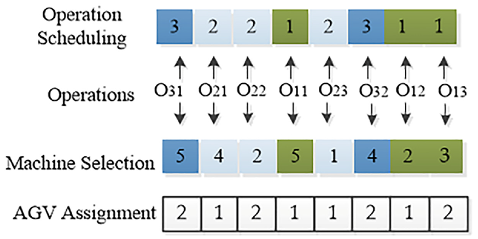
Encoding method.

A decoding method called Left Shift Insertion is used. Details of the process are as follows:

• Step1: From left to right, the chromosome genes are read and then converted into the corresponding operation O_ij, AGV w, and Machine k. In addition, the selected machine allows for the determination of the processing time P_ijk, the end time CT_ij-1k obtained to the preceding process O _ij-1 and the machine M on which the preceding process is located.

• Step2: The transport time T_v,Wi,j of the AGV operation is determined. The dual constraints of the machine and the AGV need to be considered for the decoding calculation, as shown in equations (17) and (19).

• Step3: Determine the start time and end time of the AGV operation by equations (9)–(13) and (16).

• Step4: At the same time, Processing start time ST_i,j,k are determined. The constraints of the job and the machine need to be considered for the decoding calculation, as shown in equations (6)–(8), equations (18) and (20).

• Step5: The spare time on the machining sequence is firstly traversed. Determine whether the start time of process O_ij does not exceed the completion time of the other operations in the processing queue. On the other hand, it is also determined whether the machine can process the operation during that idle time. If the above condition is satisfied, then operation O_ij is scheduled in the idle time interval for that machine. Finally, the processing sequence on the machine will be updated. Similarly, first determine whether the start time of the transportation job is earlier than other jobs in the transportation queue, and secondly determine whether the AGV can complete the task in the idle time. If the above conditions are met, the transportation job is inserted into its transportation queue. The transportation sequence on the AGV will be updated.

• Step6: Repeat step 1 to step 5 until all jobs have been machined. The start time, machine, AGV and ending time for each process are obtained for each job and the scheduling plan is generated.

Population initialization

A fine initial population not only facilitates the algorithm to search for promising regions, but also provides enough diversity to avoid premature convergence. ⁴⁰ In view of section 4.2, three vectors need to be initialized. Considering the characteristics of the scheduling problem, three strategies are designed in this section, global search (GS), allocation based on AGV scheduling (AS) rules and random scheduling (RS). Through repeated trials, the initial population is generated using the GS and AS strategies in the order of 10% and the remaining 80% in a random rule. The detailed steps are as follows.

Global search (GS)

The global minimum processing time rule ⁴¹ was introduced into the initialization to boost the quality of the solution. The concept of GS-based initialization is as follows: after assigning machines with the global minimum processing time rule, the AGV sequence is acquired using roulette selection.

Allocation based on AGV scheduling rules (AS)

In terms of machine allocation, the difference with section 4.3.1 is that the time group is set to 0 after the machines have been scheduled for all operations for each job. After assigning a machine to an operation of the job, the selection of the AGV is based on the condition that the time for the AGV to complete the transport task of the next operation is greater than the time when the next process can start processing. If all AGVs meet the condition, the earliest AGV that can complete the transport task is considered, otherwise the earliest available AGV is selected. Moreover, if more than

Algorithm 1 Procedure of initializing population by AS strategy
Input: the number of job (J), the machine array (M = {m1, m2, …, mn}), the compatible machine set for Oij (Mij) and the corresponding processing time (Tijk), the number of AGV (A), operation set (O),
Output: operation sequence OS, machine sequence MS, AGV sequence AS
OS← random sort of O respecting the process constraint % Initialize OS
Set a variation Len to record the length of OS
Set an array WT to record the total work time on the corresponding machine, WT← empty
MS← empty
for i = 1: J
for j = 1: Len
if (Oj = i)
Add the processing time corresponding to the optional machine set of the process to WT
Find the Mindex within the Mij which has the minimum max (WT), if there is more than one such Mindex, select one randomly.
MS (j) ← index
% Initialize AS
Set an array PAGV which uniformly distributed AGVs
Define a constraint C the end time node of the next process transport task is greater than the start
time of the next process
for i = 1: Len do
if all AGVs satisfy C
AS← an AGV that can be completed earliest
else if Multiple AGVs satisfy C
AS←an AGV with the smallest total load
else if
AS←an AGV with the earliest available
end for
end for
end for
return OS, MS, AS

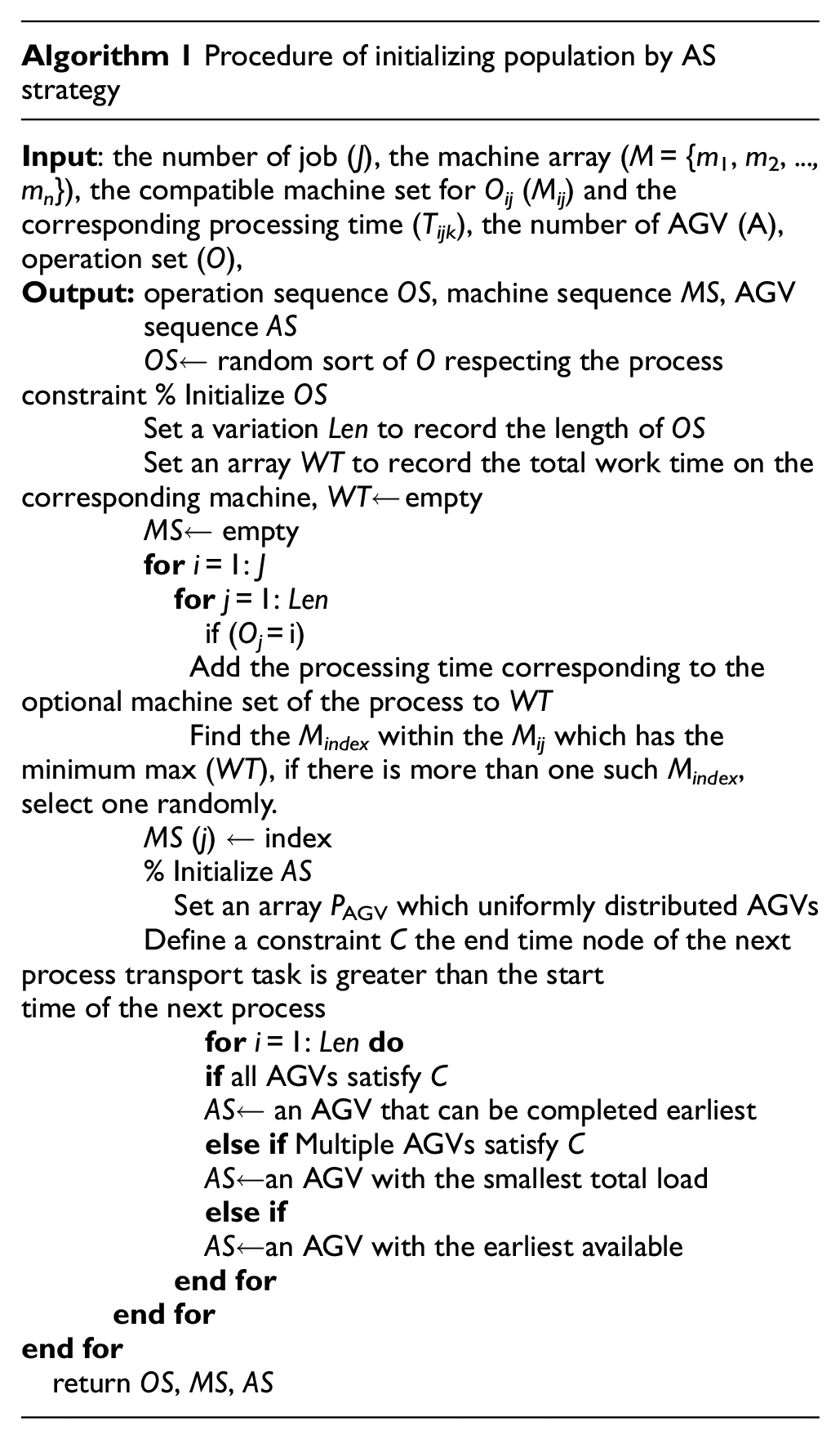
one AGV meets the condition, the AGV with the lowest current load is designated. The detailed process of the AS strategy is stated in Algorithm 2.

Random strategy

To ensure the diversity of the initial population, the processing machines and AGVs for each process of each job will be randomly selected according to the order of the jobs to generate the initial chromosomes.

Algorithmic operation operator design

Selection

For two chromosomes, the better chromosome has a greater chance of being selected. In this paper, two individuals are randomly selected for comparison at a time, and the individual with the higher non-–dominance ranking is selected. If two solutions are of equal rank, the individual with the greater crowding distance is favored.

Crossover

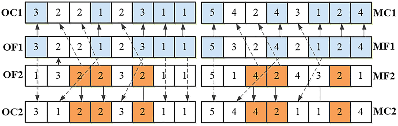
According to the characteristics of the research problem in this paper, IPOX crossover ⁴² is used for the gene string based on process coding, which can well succeed the superior characteristics of its parents. However, if only the operation ordering vector is cross–genetically manipulated, there is a high probability of illegal solutions. To accommodate the coding strategy in section 4, the machine assignment vector should be transformed accordingly during the cross-over process. Since all AGVs are available for each operation, the task vector of the AGV does not need to be adjusted. The IPOX crossover is illustrated in Figure 3 (four parents are noted as OF1, OF2, MF1, and MF2; four offspring are noted as OC1, OC2, MC1, and MC2). Take the workpiece processing information in Table 4 as an example. First divide all the workpiece machines into two random sets J1 = {j1, j3} and J2 = {j2}, copying the workpieces contained in OF1 from J1 to OC1 and OF2 from J2 to OC2, retaining their position. Copy OF2 containing the artifacts in J2 to OC1 and OF1 containing the artifacts in J1 to OC2, retaining their order. The machine code is transformed accordingly during the crossover.

Figure 3.

POX crossover procedure.

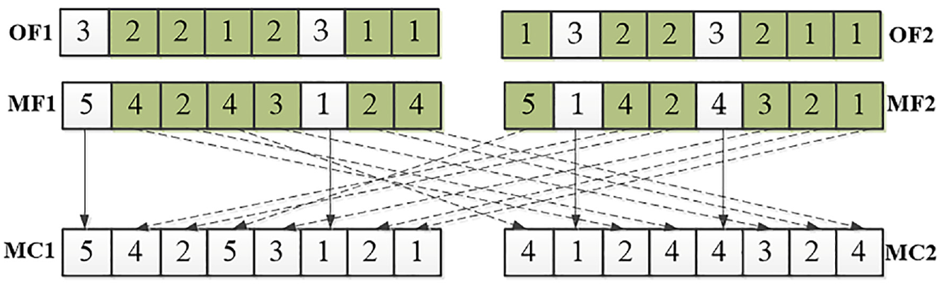
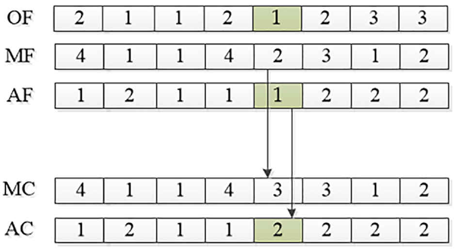
Improved MPX crossover is used for the machine assignment vector. Take the job processing information in Table 4 as an example. First, the jobs such as {J1, J2} (i.e. number 1 in OF1 and number 2 in OF2) are selected from the job set J and their positions of occurrence in OF1, OF2 are recorded. The unrecorded genes in the parent MF1 and MF2 were placed in the offspring MC1, MC2, respectively, as shown in Figure 4. Finally, the machine genes of the same process in MF1 and MF2 are exchanged and inserted sequentially into the corresponding positions of the offspring. The crossover of AGV chromosomes was not considered.

Figure 4.

MPX crossover procedure.

Mutation

The mutation causes random changes in chromosomes and thus increases the diversity of the population. In this paper, machine, and AGV mutations are based on machine coded and AGV coded chromosomes. Machine mutation is the process of selecting a new machine from a set of alternative machines for an operation to replace the current machine of the operation. The AGV is mutated in a similar manner to machine mutation. As shown in Figure 5, operation O13 is randomly selected. When mutation occurs, machine M1 is selected to replace the current machine M4 of the process. At the same time, select AGV No. 2 to replace the assigned AGV No. 1.

Figure 5.

Mutation procedure.

Elite strategy

In this section, an improved elite retention strategy is designed. By introducing a distribution function to prevent the population from converging in advance or converging with the local optimal solution. The function is established as formula (20), where j is the non-dominated rank. |F_j| denotes the number of individuals on the jth non-dominated surface.

$$n_j=|F_j|\times r_j$$

(20)

nj denotes the number of individuals selected on the non-dominated surface Fj at level j and r_j is a random number between 0 and 1. The elite strategy are as follows.

• Step1: Initialize the elite pool Pt, which is equal to the harmony memory library size (HMS), and set t = 0.

• Step2: The merged population is calculated using the fast non-dominated sorting and the crowding distance for all individuals of the populations, and the R_j non-dominated rank surface F = {F₁······F_j} was constructed according to the pareto concept.

• Step3: Clear P_t+ 1 and set i = 1.

• Step4: If |P_t +  ₁ |+|ni|>HMS, then continue to Step5, Otherwise, skip to Step6.

• Step5: The crowding distances of the individuals in F_j are calculated and sorted by crowding distance and the individuals in F_j are added to P_t + 1.

• Step6: i = i + 1, the program returns to Step4.

Improvising new harmony

The generation of new harmony is the core of the HS algorithm. To improve the quality of the harmony, a neighborhood-based local search is proposed. In general, a neighborhood structure design based on problem knowledge (e.g. critical path) can improve algorithm search efficiency. Therefore, the method of obtaining critical paths in previous studies was first adopted. ⁴³ Then, two critical path-based neighborhood search operators are described.

Local search operator 1

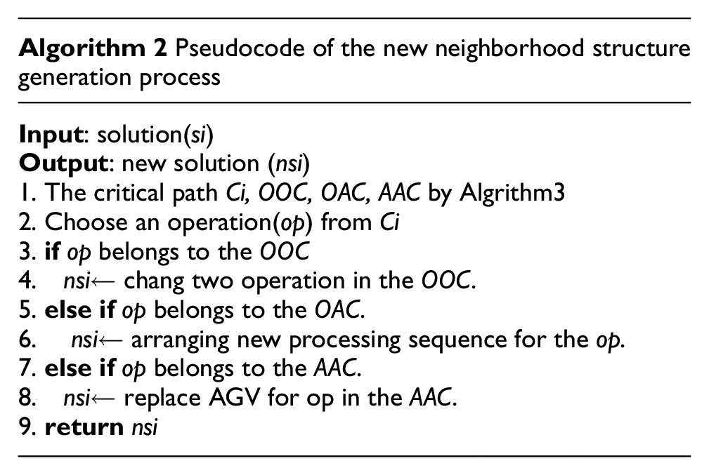
Analysis of two operations on a critical path reveals that the latter operation is delayed by the former. In fact, the impact of the job processing process and the limitations of resources (e.g. machines and AGVs) are the reasons for delays in the overall process. Here, the AGV operation can be considered as a processing operation. The three delay reasons correspond to the three connection methods on the analytical diagram respectively. An operation-operation connection (OOC) means that when a job arrives at the target machine, the machine is occupied. When the AGV reaches the destination machine but does not leave immediately, operation-AGV connection (OAC) is created. In addition to the above, cases where the processing process is limited by AGV resources are represented on the parsing diagram as an AGV-AGV connection (AAC). In Figure 6 these connections can be further explained. The critical operations {O23, O11}, and {{T32, T11}, {T32, T21}} are classified as OOC and AAC respectively. Based on these connection cases, three neighborhood structures are designed, and the pseudocode generated by the neighborhood structure is described in Algorithm 4.

Figure 6.

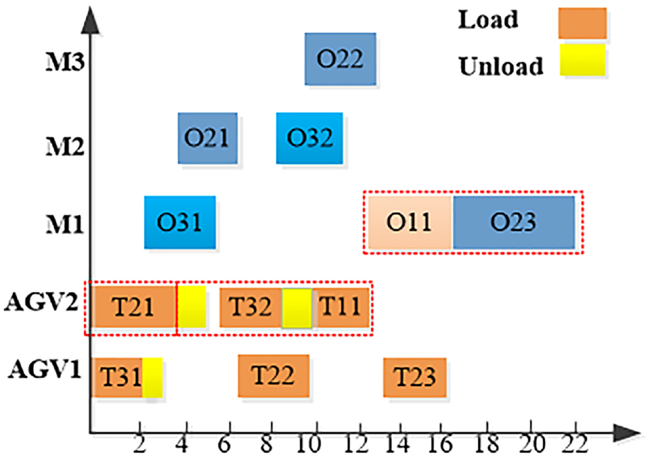
Gantt chart.

Algorithm 2 Pseudocode of the new neighborhood structure generation process
Input: solution(si) Output: new solution (nsi) 1. The critical path Ci, OOC, OAC, AAC by Algrithm3 2. Choose an operation(op) from Ci 3. if op belongs to the OOC 4. nsi← chang two operation in the OOC. 5. else if op belongs to the OAC. 6.  nsi← arranging new processing sequence for the op. 7. else if op belongs to the AAC. 8. nsi← replace AGV for op in the AAC. 9. return nsi

Local search operator 2

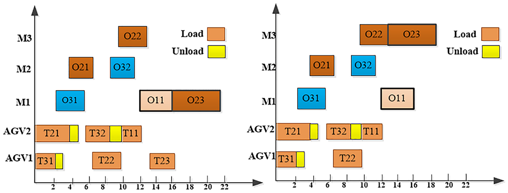
Critical operations are shifted to machines with lower workload, which increases the possibility to generate better scheduling ⁴⁴ The selection of critical operations is determined by the metric R. R is the ratio of the processing time of an operation to the number of operations in its corresponding job. As is illustrated in Figure 7, the most heavily loaded machine is the M1, and the critical operations on the M1 are O11 and O23 respectively. However, O11 is not considered and only O23 is allocated to the machine with the least load in its optional machine set. It is clear that the dispatch completion time has been reduced from 22 to 18 s. Therefore, this neighborhood search not only allows the machine load to be balanced, but also allows the workload of the AGV to be reduced. The detailed steps are as follows:

• Step1: Set up a temporary array S that stores the critical operation metric value R and an array M_i that records all machine loads, the size of which is m.

• Step2: Calculate the loads of all machines and record them in the array M. The array M is arranged in descending order, and the corresponding machine indices are also arranged accordingly.

• Step3: t = 0, calculate the R value of the critical operation on the machine corresponding to the array M_t in order, and skip it if the process is the initial process of the job. Otherwise, and record its R value in the array S.

• Step4: The array S is first arranged in descending order. Then the critical operation corresponding to the array S is traversed to find the free time interval on the machine available for that process. Finally, when the previous operation of the critical operation is completed, the critical operation is inserted into the appropriate free interval.

• Step5: If the new solution dominates the old one, the old one is replaced. Go to step 4 until all operations corresponding to the array S have been processed.

• Step6: t = t + 1, if t = m, then stop. Otherwise skip to Step 3.

Figure 7.

Example of local search operator.

Smart mutation of harmony

To prevent local search from getting stuck in local optimum due to its high convergence, intelligent mutation operation on new harmony is designed. The smart mutation of harmony as follows.

• Step1: If the random probability rand <MP (MP denotes the intelligent mutation probability), the new harmony satisfies the mutation condition.

• Step2: After decoding the harmony, the machine and AGV with the largest load are counted, named M and W respectively.

• Step3: First, an operation is randomly selected from the machine M, and then a new machine is selected from the optional machine set of the operation to replace M. If there is only one machine available for the operation, go back to Step2. Similarly, the corresponding AGV is replaced with another AGV.

Update harmony memory

In the proposed algorithm, the new harmony generated in Section 3.5 is merged with the original harmony memory library. The merged population undergoes non-dominant sorting and crowding computations, using the elite strategy in Section 3.4 to update the harmony memory library.

Numerical experiments

This section focuses on verifying the behavior of the proposed algorithm. Three metrics and instances for evaluating the performance of the solution set are first described. Then the parameters in the algorithm are calibrated. Finally, comparative experiments are performed in this section. All the experiments were conducted on a PC equipped with an Intel Core i7, 2.30 GHz, 16 GB of RAM, and Windows 10. Furthermore, all experiments are implemented in C++ coding in visual studio2019 software.

Evaluation indicators and instances

The optimal solution of multi-objective is not unique and it is impossible to judge the merit of the feasible solution, so the results obtained by the algorithm need to be evaluated from several aspects. In this article, the results obtained are evaluated according to the following three commonly used metrics.

1. SP is an evaluation metric proposed in the literature ⁴⁵ as the variance of the distance between neighboring solutions in the non-dominated solution set. If SP value is smaller, the better the distributivity of the solution set obtained by the algorithm is.

2. The spread of non-dominated solutions (SNS), ⁴⁶ a metric that decides the diversity of the non-dominated solution set. The higher the SNS value is, the better the diversity of solutions is.

3. 3.The mean ideal distance (MID), ⁴⁷ which indicates the proximity between the pareto solution and the ideal point (0,0,0), implies that the lower the MID value is, the better the quality of the solution is.

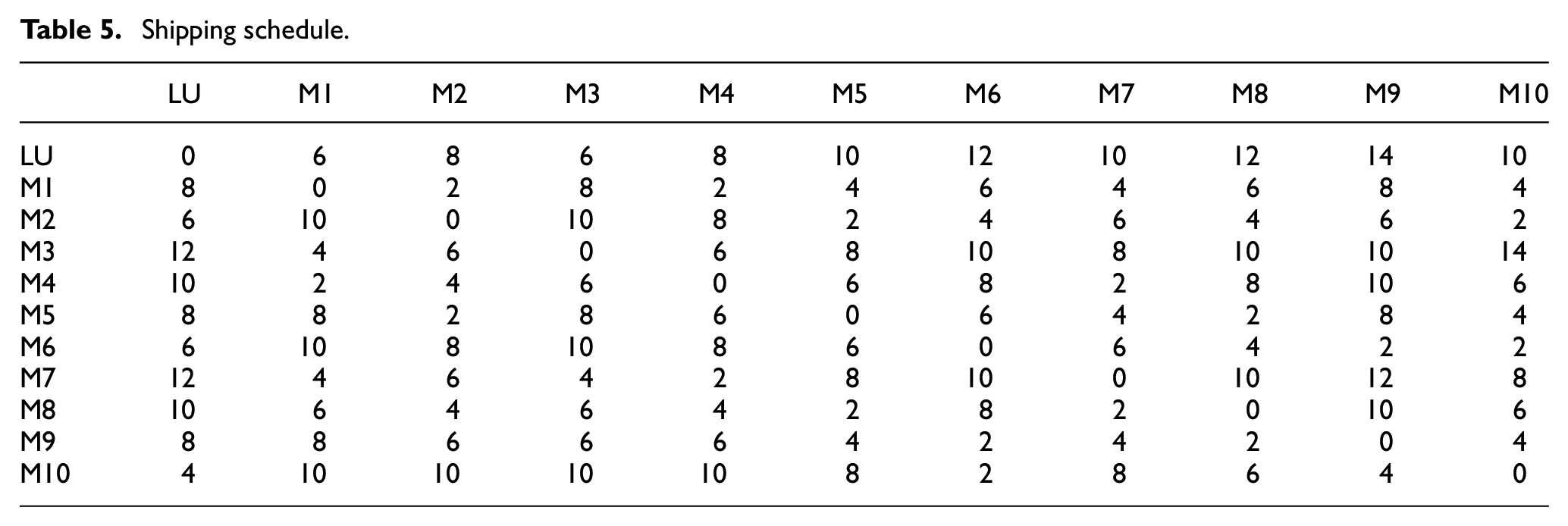
In this section, Deroussi and Norre ¹⁹ instances are used to test the single-objective aspect of the solution. In addition, new instances are generated by modifying the machine layout in Deroussi and Norre ¹⁹ according to Kacem et al. ⁴⁸ Figure 8shows the layout of the workshop machines, where M1 represents machine 1, and so on. The corresponding transportation schedule is illustrated in Table 5.

Figure 8.

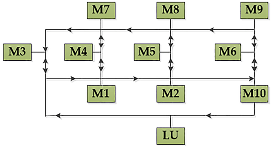
Machine layout

Table 5.

Shipping schedule.

	LU	M1	M2	M3	M4	M5	M6	M7	M8	M9	M10
LU	0	6	8	6	8	10	12	10	12	14	10
M1	8	0	2	8	2	4	6	4	6	8	4
M2	6	10	0	10	8	2	4	6	4	6	2
M3	12	4	6	0	6	8	10	8	10	10	14
M4	10	2	4	6	0	6	8	2	8	10	6
M5	8	8	2	8	6	0	6	4	2	8	4
M6	6	10	8	10	8	6	0	6	4	2	2
M7	12	4	6	4	2	8	10	0	10	12	8
M8	10	6	4	6	4	2	8	2	0	10	6
M9	8	8	6	6	6	4	2	4	2	0	4
M10	4	10	10	10	10	8	2	8	6	4	0

Parameter setting

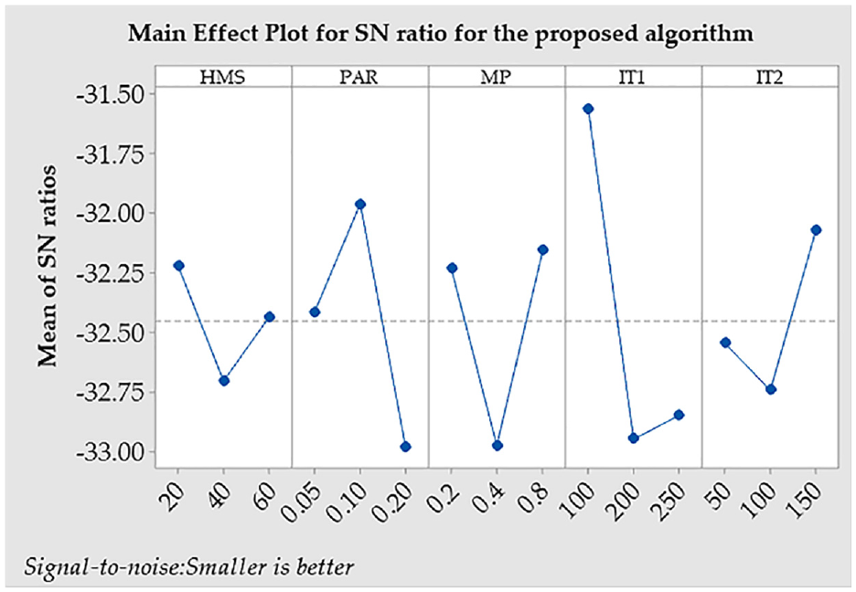
Appropriate algorithm parameters can boost algorithm behavior. Total iterations IT₁, harmony iterations IT₂, the HMS, fine-tuning probability PAR, and the probability of the mutation of the harmony intelligence MP are significantly relied on to obtain a better objective value. To explore the impacts of parameters on algorithm performance, the MiniTab software is used as a tool and the L27 orthogonal array design was chosen to implement the Taguchi method. ⁴⁹ Taking the average ideal distance (MID) as the evaluation standard, the ideal point is set to (0, 0, 0), and the example FJSP5 of Deroussi and Norre ¹⁹ is used for experiments. The smaller the MID value is, the better the parameter combination is. Finally, each combination was run 10 times independently and the mean is calculated. The changing trend of each factor level is shown in Figure 9. Therefore, it can be determined that HMS, PAR, MP, IT1, and IT2 are set to 20, 0.1, 0.4, 100, and 150, respectively.

Figure 9.

Trends of each factor level.

Comparison experiment

Comparison of single-objective Deroussi instances

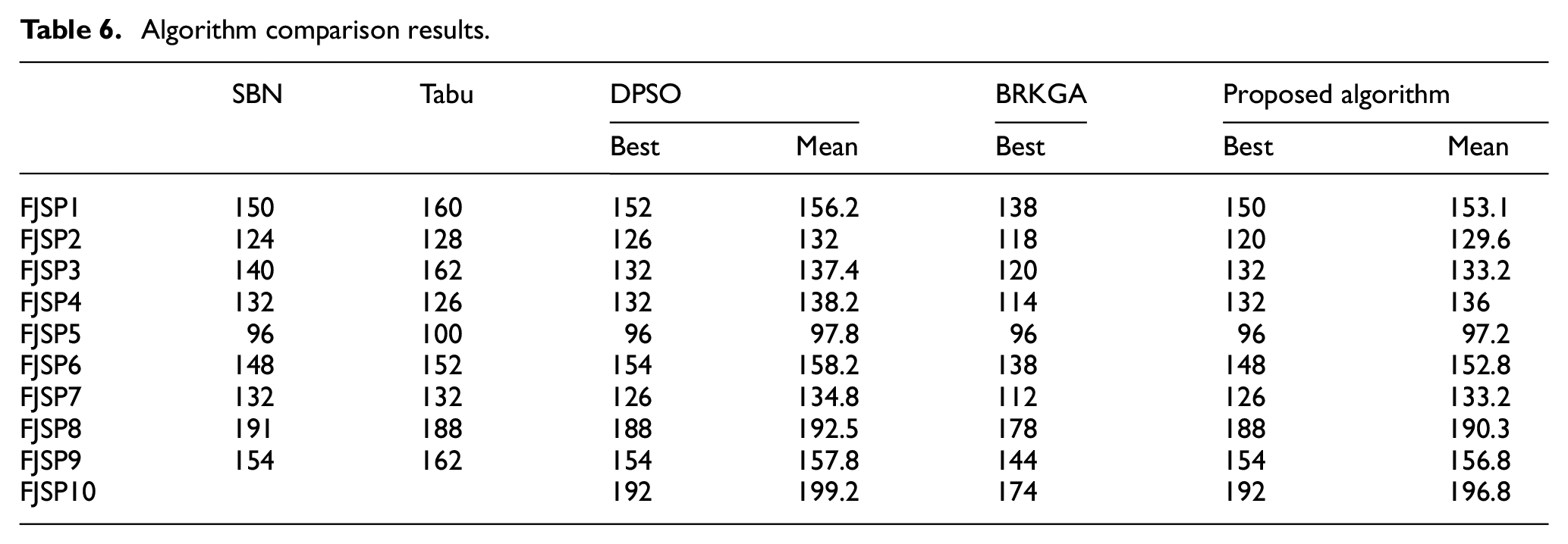
To check the effectiveness of the proposed algorithm, experiments were implemented with the objective of minimizing the makespan. Twenty experiments were carried out on 10 cases respectively. The experimental results are compared with DPSO, ⁴⁹ Tabu ⁵⁰ SBN, ²¹ and BRKGA. ²⁷ The optimal solution and average value of makespan are shown in Table 6. The above comparison algorithms are all single-objective algorithms with the maximum completion time as the goal, compared with the multi-objective algorithm in this paper. The results in Table 6 show that, except for FJSP4, the makespan calculated by the proposed algorithm are superior to or equivalent to the results of the Tabu, SNS, and DPSO. However, the results are slightly worse when compared to BRKGA. Therefore, the proposed algorithm is still efficient and feasible when applied to resolve the same case. Figure 10. shows the scheduling solution for FJSP2 with a makespan of 120. The green box indicates the AGV handling process assigned to each operation and the yellow box represents the AGV is unloaded.

Table 6.

Algorithm comparison results.

	SBN	Tabu	DPSO		BRKGA	Proposed algorithm
			Best	Mean	Best	Best	Mean
FJSP1	150	160	152	156.2	138	150	153.1
FJSP2	124	128	126	132	118	120	129.6
FJSP3	140	162	132	137.4	120	132	133.2
FJSP4	132	126	132	138.2	114	132	136
FJSP5	96	100	96	97.8	96	96	97.2
FJSP6	148	152	154	158.2	138	148	152.8
FJSP7	132	132	126	134.8	112	126	133.2
FJSP8	191	188	188	192.5	178	188	190.3
FJSP9	154	162	154	157.8	144	154	156.8
FJSP10			192	199.2	174	192	196.8

Figure 10.

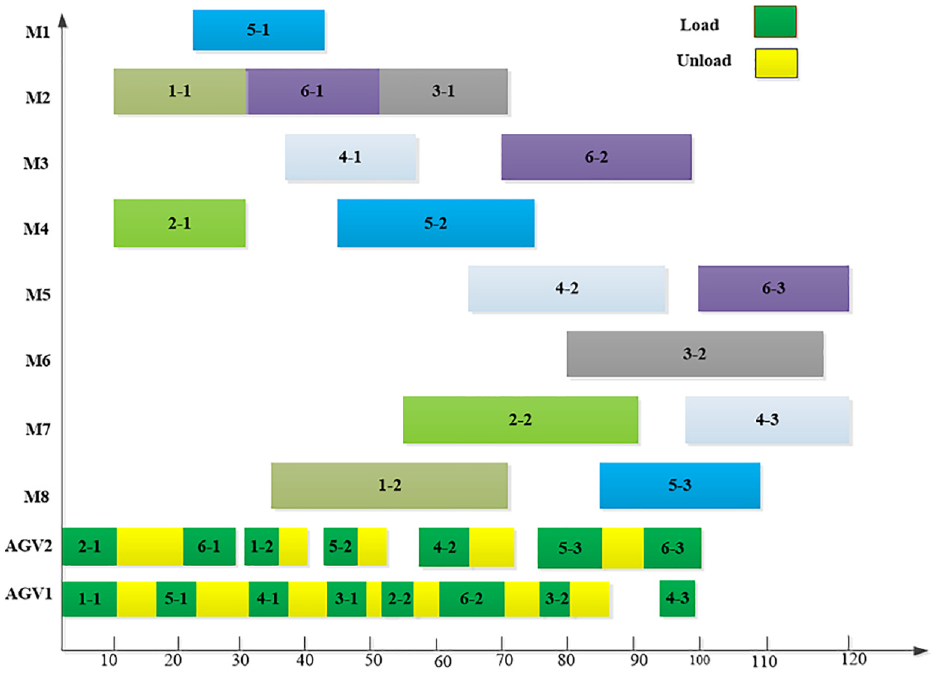
FJSP2 scheduling Gantt chart.

Comparison of multi-objective algorithms

Analysis of the effectiveness of improvement strategies

To inspect the practical function of each improved strategy on the global algorithm, two variants of NSGA-II are designed in this section. NSGA-II is the classic edition without any improved strategy. NSGA-II-1 adoptes the population method and NSGA-II-2 combines the neighborhood search techniques proposed in this paper. For each instance, each algorithm is run 20 times independently. Table 7 shows the mean of 20 results. In terms of SP on the 16 problems scales, NSGA-II, NSGA-II-1, and NSGA-II-2 won 1, 8, and 7, respectively. For SNS, NSGA-II, NSGA-II-1, and NSGA-II-2 won 1, 3, and 12, respectively. Considering the MID metric, NSGA-II, NSGA-II-1, and NSGA-II-2 won 1, 5, and 10, respectively. All the results demonstrate that NSGA-II-1 and NSGA-II-2 are better than NSGA-II in solving performance, which means the effectiveness of the initialization method and neighborhood search strategy proposed in this paper.

Table 7.

experimental results.

Instance	AGV Number	NSGA-II			NSGA-II-1			NSGA-II-2
		SP	SNS	MID	SP	SNS	MID	SP	SNS	MID
fjspT3-4	2	3.1	2.7	7.7	2.7	3	9.2	4	2.3	6.3
fjspT4-5	2	8.8	2.6	11.7	3.6	3.2	8.6	4	3.8	9.8
	3	7.4	2.6	12.3	3.5	3.1	8.4	3.4	3.8	9.5
fispT8-8	2	7.6	4.2	9.6	5.1	5.2	13.9	4.4	6.3	16.1
	3	6.1	4.7	17.4	4	5	16.2	6.9	5.5	14.9
	4	7.2	4.3	18	7	5	14.3	6.6	5.8	14.9
fjspT10-7	2	6.2	5.2	20	3	5.8	18	3.4	6.6	12.1
	3	5.7	4	17	6.4	5.3	13.7	3.5	5.7	17.8
	4	5.2	4.4	17.1	7.1	4.4	14.8	5.5	5.6	13.2
fjspT10-10	2	6.5	5.7	21.2	3.3	5.9	12.8	3.4	6.6	13
	3	8.7	4.4	19.9	6	5.2	15.1	7.7	6.4	15
	4	6.9	4.7	19.7	7	4.7	16.1	6.3	6.3	14.2
fjspT15-10	2	9	8.1	24.3	2.3	8.2	21.4	4.4	7.9	20
	3	8.1	6.3	23	9	7	21.2	4	7.6	18.3
	4	7.4	8.7	26	9.2	9.9	30	3.4	8.7	17.8
	5	4.6	7.9	24	2.6	8.6	20.8	4.5	8	16.9
WIN(Rate)		6%	6%	6%	50%	19%	32%	44%	75%	62%

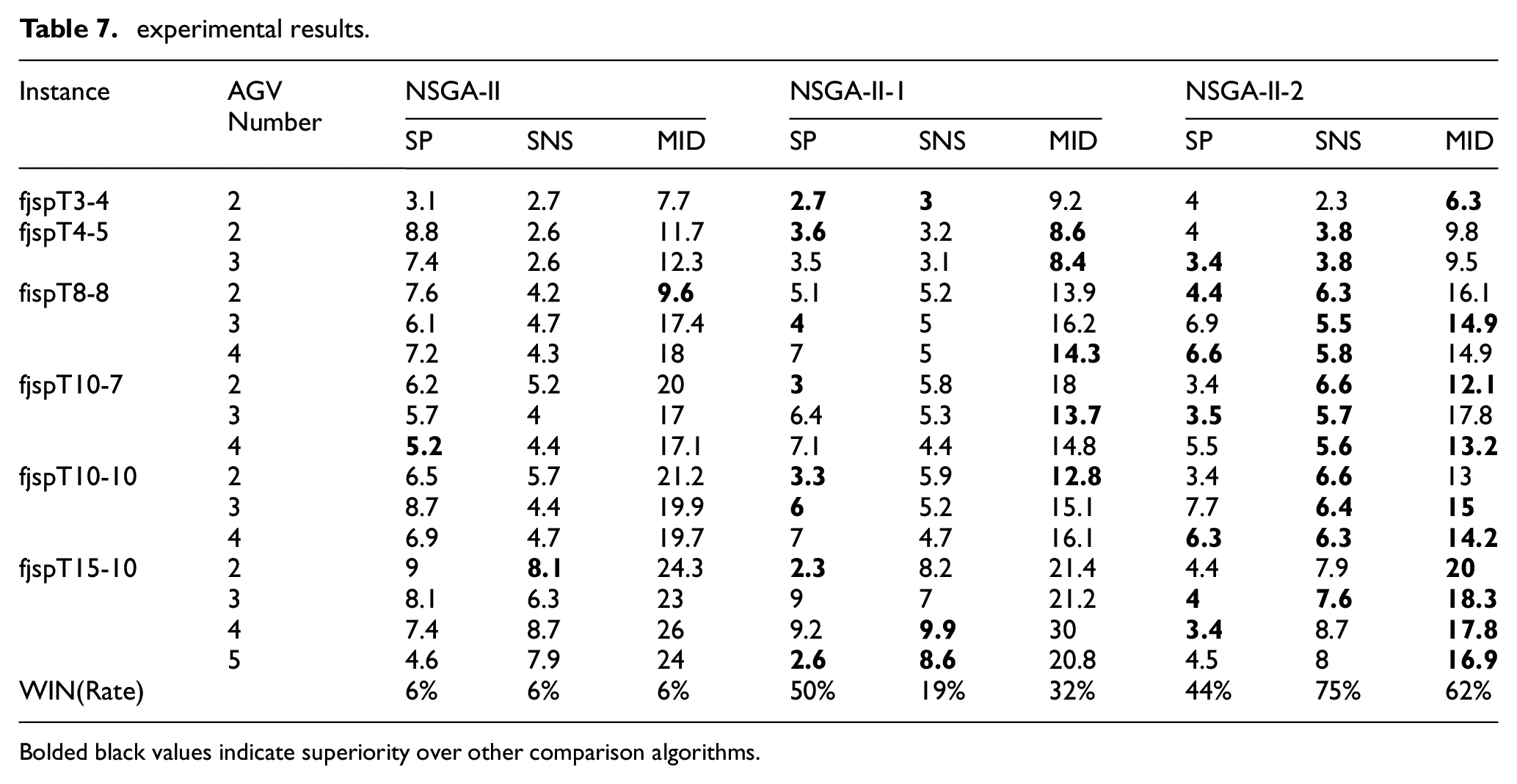
Bolded black values indicate superiority over other comparison algorithms.

To reflect the discrete distribution of the data in Table 5, we plotted the data as a boxed line graph, as is shown in Figure 11. In terms of SP indicators, the box corresponding to the improved algorithm is longer, indicating that the concentration of SP indicators obtained from NSGA-II-1 and NSGA-II-2 is slightly less. However, there is a significant decrease in the MID indicator and a significant upward trend in the SNS indicator. In summary, the improved algorithm has better performance.

Figure 11.

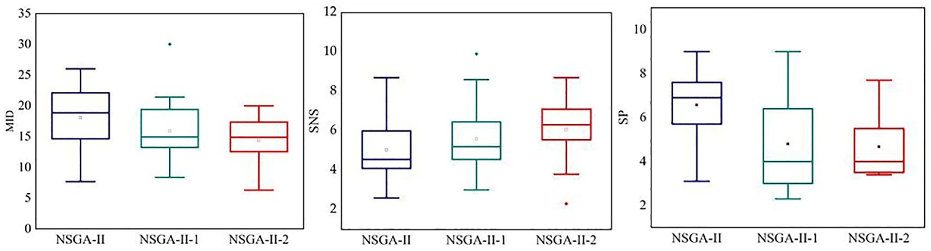
Box plots for MID, SNS, and SP.

To further evaluate the effectiveness of the two improvement strategies, the large-scale example fjspT10-7 was selected and tested with three and four AGV carts. The solutions obtained are presented in Figure 12(a) and (b). And it can be found that both NSGA-II-1 and NSGA-II-2 obtain better solutions than the classical NSGA-II. It is also demonstrated that the strategy can help to achieve global optimality by generating high-quality initial solutions in the case of multiple AGVs working with rational AGV scheduling rules. In summary, the improved strategy notably ameliorates the performance of the algorithm in terms of convergence quality and synthesis quality.

Figure 12.

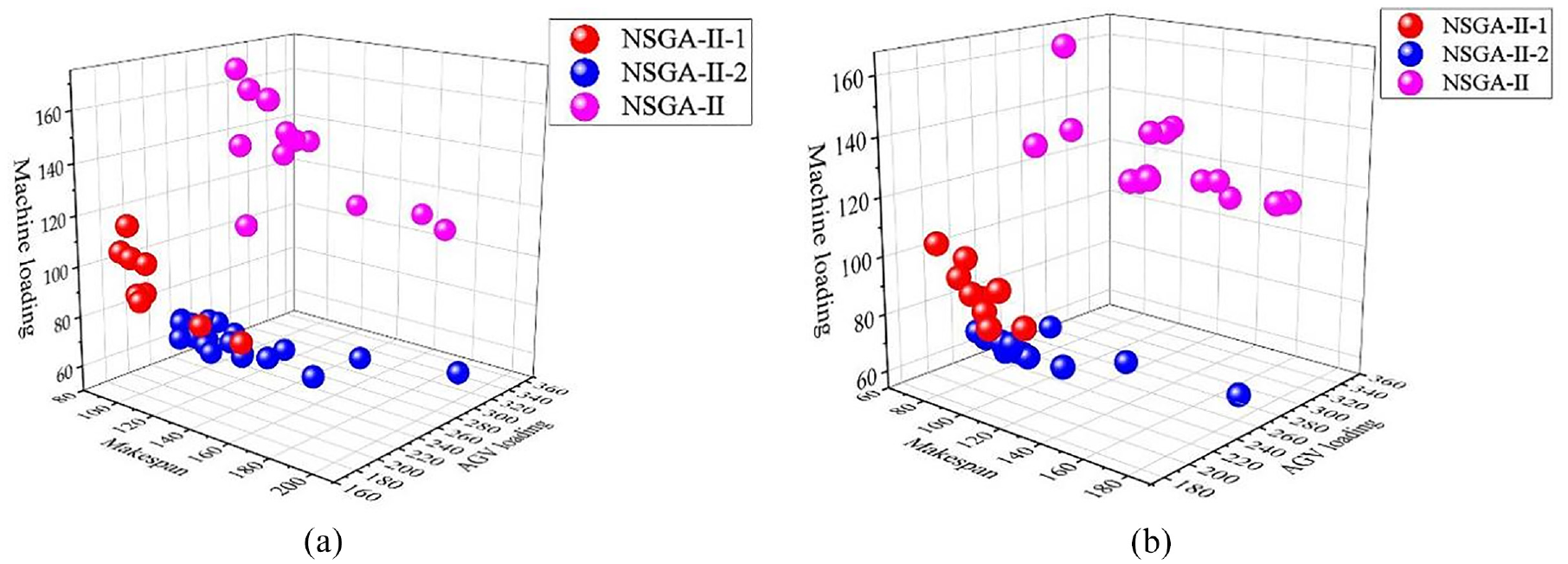
(a). Pareto fronts gained by the NSGA-II, NSGA-II-1, and NSAG-II-2 in the case of three AGVs, (b). Pareto fronts gained by the NSGA-II, NSGA-II-1, and NSAG-II-2 in the case of four AGVs.

Comparison of the proposed algorithm with NSGA-II, SPEA2 and MOPSO

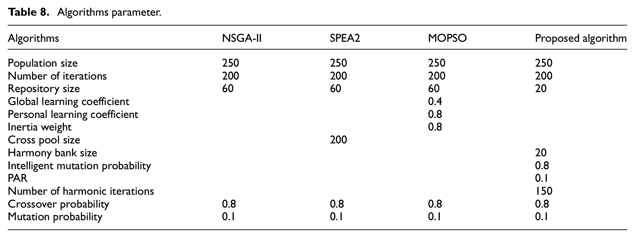
To validate the advantages of the proposed algorithm in solving multi-objective problems. NSGA-II, MOPSO, and the Strength Pareto Evolutionary Algorithm (SPEA2) are used as comparison algorithms in this paper. NSGA-II and SPEA2 are popular multi-objective evolutionary algorithms that have been successfully applied in many fields. In addition, MOPSO uses a Pareto-based method for finding the optimum, and both NSGA-II and SPEA2 both use a binary tournament selection strategy. The various algorithm parameters are set as shown in Table 8, where all common parameter settings are configured to the same value. The parameters affect the optimization ability of the algorithm. Considering the fairness of the experiment, this paper iteratively uses Taguchis experimental method to determine the parameter values of each algorithm.

Table 8.

Algorithms parameter.

Algorithms	NSGA-II	SPEA2	MOPSO	Proposed algorithm
Population size	250	250	250	250
Number of iterations	200	200	200	200
Repository size	60	60	60	20
Global learning coefficient			0.4
Personal learning coefficient			0.8
Inertia weight			0.8
Cross pool size		200
Harmony bank size				20
Intelligent mutation probability				0.8
PAR				0.1
Number of harmonic iterations				150
Crossover probability	0.8	0.8	0.8	0.8
Mutation probability	0.1	0.1	0.1	0.1

Consider the algorithm to have a certain randomness, each algorithm is run 20 times independently for each case. The test results are exhibited in Table 9. The bolded parts indicate that the results of this paper are superior to other comparison algorithms under the same instance. It was glaringly obvious that the proposed algorithm achieves better MID, SP, and SNS performance in all cases.

Table 9.

Experimental performance of the four multi-objective algorithms for SP, SNS, and MID.

Instance	AGV number	NSGA-II			SPEA2			MOPSO			Proposed algorithm
		MID	SP	SNS	MID	SP	SNS	MID	SP	SNS	MID	SP	SNS
fjspT3-4	2	7.7	3.1	2.7	12.7	2.0	4.1	7.0	2.8	2.0	4.3	1.8	8.5
fjsp4T-5	2	11.7	8.8	2.6	9.2	7.6	3.0	8.5	8.7	2.5	6.0	3.7	7.7
	3	12.3	7.4	2.6	7.7	6.2	2.6	8.0	9.0	2.4	8.4	5.7	7.1
fispT8-8	2	9.6	7.6	4.2	19.0	9.9	6.2	15.4	9.0	4.7	6.7	5.0	12.7
	3	17.4	6.1	4.7	21.3	6.4	7.0	16.1	9.8	4.8	9.9	3.6	9.9
	4	18	7.2	4.3	19.2	7.0	6.4	16.5	7.0	5.0	14.0	5.6	9.8
fjspT10-7	2	20	6.2	5.2	21.7	5.4	7.1	15.0	9.2	4.6	14.4	6.0	10.8
	3	17	5.7	4	22.5	7.7	7.3	13.5	8.0	4.1	11.6	4.1	8.3
	4	17.1	5.2	4.4	19.0	5.0	6.2	16.6	9.6	5.0	16.0	3.0	9.0
fjspT10-10	2	21.2	6.5	5.7	21.3	6.6	6.9	17	7.5	5.2	14.0	5.9	10.2
	3	19.9	8.7	4.4	19.2	5.2	6.2	14.4	7.6	4.4	11.7	4.6	9.6
	4	19.7	6.9	4.7	17.9	6.8	5.9	14.0	9.7	4.2	12.3	6.3	8.1
fjspT15-10	2	24.3	9	8.1	35.9	6.5	11.6	18.1	13.1	5.1	14.7	5.0	18.0
	3	23	8.1	6.3	32.5	6.2	10.7	21.3	18.0	6.4	21	2.8	18.7
	4	26	7.4	8.7	34.4	5.7	11.3	16.4	16.0	5.0	15.5	4.3	12.9
	5	24	4.6	7.9	31.0	7.3	10.1	16.3	16.7	4.8	15.8	4.0	13.9

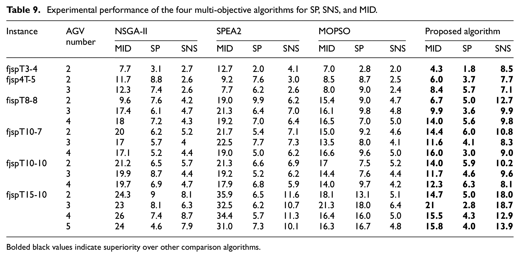
Bolded black values indicate superiority over other comparison algorithms.

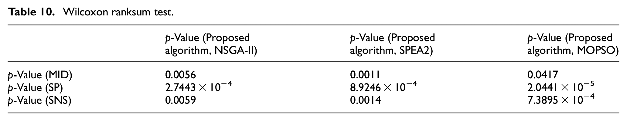
A nonparametric test using the Wilcoxon’s rank sum test is performed to test whether there is an obvious difference in the results among the four algorithms. Combined with the data in Table 10, the statistical results between the proposed algorithm and the other algorithms are all less than 0.05, indicating superiority over the other comparison algorithms from a statistical point of view.

Table 10.

Wilcoxon ranksum test.

	p-Value (Proposed algorithm, NSGA-II)	p-Value (Proposed algorithm, SPEA2)	p-Value (Proposed algorithm, MOPSO)
p-Value (MID)	0.0056	0.0011	0.0417
p-Value (SP)	2.7443 × 10−4	8.9246 × 10−4	2.0441 × 10−5
p-Value (SNS)	0.0059	0.0014	7.3895 × 10−4

In addition, the largest case of fjspT15-10 with a number of AGVs of 5 is selected for experiments to compare the performance of the MOPSO, NSGA-II, and SPEA2 with the algorithm in this paper. The average convergence curves of the objective functions of the four algorithms are displayed in Figure 13. The figures view that the proposed algorithm converges quickly and overcomes the premature convergence of MOPSO, SPEA2, and NSGA-II for solving MA-FJSP problems.

Figure 13.

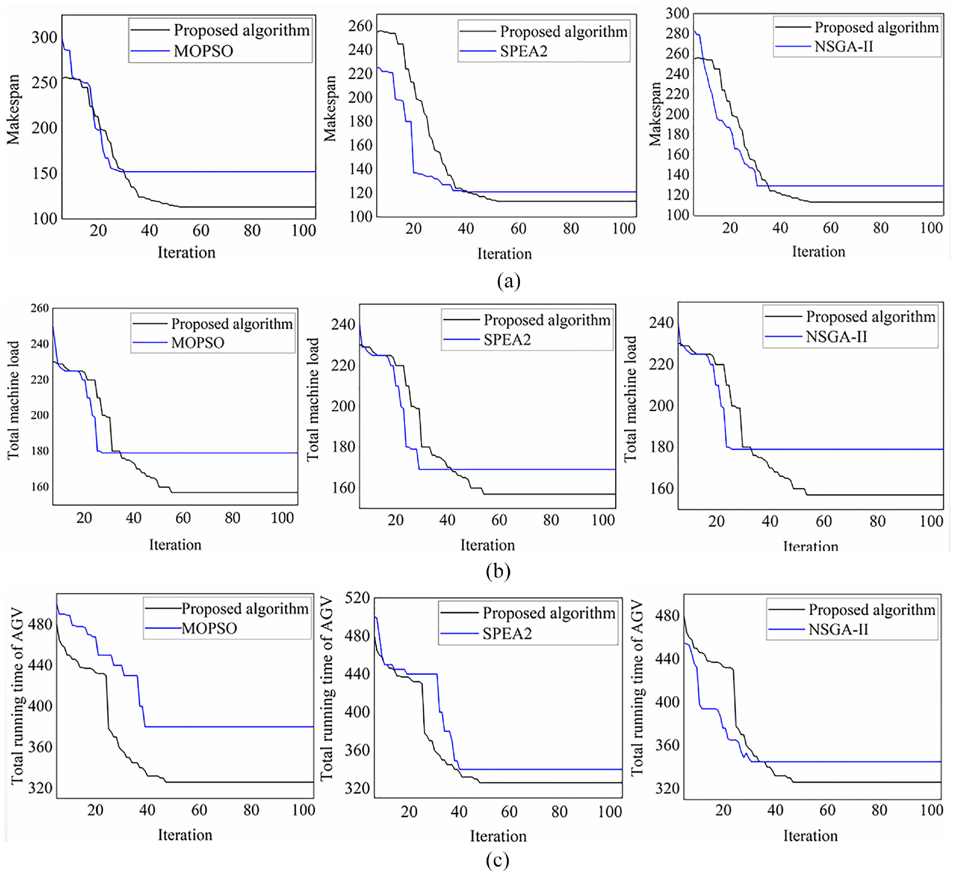
(a) Convergence curves of makespan for each algorithm; (b) Convergence curves of total machine load for each algorithm and (c) Convergence curves of total running of AGV for each algorithm.

Conclusion and outlook

In this paper, makespan, total AGV runtime, and total processing machine load are used as performance criteria. A hybrid algorithm based on the NSGA-II and the harmony search algorithm is designed to solve MA-FJSP. In the algorithm, a rule-based hybrid initialization strategy is designed to enhance the quality of the initial population. Furthermore, the causes of processing process delay are analyzed, a neighborhood search based on problem knowledge is designed. Finally, the proposed algorithm is validated by a well-known benchmark. Results of the experiment display that the effectiveness of the algorithm in solving the MA-FJSP problem, especially when the size increases.

In future work, we will explore more complex shop floor scheduling issues such as distributed shop floor scheduling environments in the context of green manufacturing. From the methodology, the mechanism of reinforcement learning will be investigated and combined with heuristics to enhance the efficiency of the solution.