This paper studies performance recovery problem of a class of uncertain nonaffine strict-feedback systems with mismatched uncertainties. First, the strict-feedback nonaffine system with mismatched system dynamics is transformed into an integrator-chain nonaffine system by a diffeomorphism. Second, the transformed system is converted to an affine one by constructing an auxiliary control input term, and dynamical uncertainties and external disturbances are viewed as total disturbance of the affine system. Then, a two-time-scale active disturbance rejection controller (ADRC) is designed for the transformed affine system. Under some mild assumptions, it can be proved that the proposed ADRC-based closed-loop system can achieve performance recovery and weak performance recovery in different cases of mismatched system dynamics, respectively. Experimental results on a magnetic levitation ball system demonstrate the effectiveness of the proposed control scheme.
Almost all physical systems are ubiquitously affected by uncertainties, which have two basic sources: internal uncertainties (parametric variations or unmodelled dynamics) and external disturbances. It is a significant issue to ensure desired performance of control systems with various uncertainties in control science and control engineering.1
Because of its ability in dealing with uncertainties effectively, simplicity in engineering implementation, and superior performance in practical application, active disturbance rejection control (ADRC) is becoming a popular control method in control engineering.2–4 It has been proved to be successful in many industrial applications in last two decades, such as fan control in server,5 position tracking and attitude control of quadrotors6 and fuel cell temperature control.7 Compared to its broad industrial applications, the rigorous theoretical analysis for ADRC ever faced great difficulties and lagged far behind for quite some time. Most notably, the significant progress has been made in novel design, rigorous and comprehensive analysis of ADRC in recent years.8–11
The aforementioned researches mainly concentrated on affine-in-control systems characterized by the control inputs appearing linearly in the state equation. However, there are limited research works on nonaffine-in-control systems, which represent some typical systems in practical applications, such as chemical reactor,12 the inverted pendulum,13 some flight control systems14 and magnetic levitation system.15
Up to present, various approaches for uncertain nonaffine systems have been proposed.16–23 An output feedback controller is designed for uncertain nonaffine systems by combining neural network observers with approximate dynamic inversion (ADI).16 By using neural networks to estimate the uncertainties and nonaffine nominal model, stability property of the overall system can be proved.17,18 An observer-based adaptive fuzzy method is proposed to control an uncertain nonaffine feedback linearization system.19 And an adaptive fuzzy controller is developed for a class of uncertain nonaffine feedback linearization systems by utilizing the passivity theorem.20 Nevertheless, these neural-network-based or fuzzy-system-based methods usually lead to heavy computation burdens and need good prior knowledge of the system.
To handle heavy computation burdens brought by the neural networks, an extended high-gain observer (EHGO) is used to estimate system states and uncertainties, and ADI is employed to handle the nonaffine inputs by using the estimates provided by EHGO.21 Based on the control method for feedback linearization systems,21 a novel control design, combining a nonlinear extended state observer (NLESO) and ADI, is proposed for uncertain nonaffine strict-feedback nonlinear systems.22 The mismatched or unobservable system dynamics is required to be known and continuously differentiable, which is a strong assumption. And only the stabilization problem is considered. A novel indirect dynamic inversion (IDI) approach is proposed for uncertain nonaffine strict-feedback nonlinear systems.23 However, the estimate of the model uncertainties offered by EHGO is not utilized, and the initial states are required to be known. If the mismatched or unobservable system dynamics are not accurately known, only weak performance recovery is achieved. A linear robust control method by combining reduced-order linear extended state observer (RLESO) and ADI, is proposed for a class of uncertain nonaffine strict-feedback nonlinear systems.24
To sum up, there are a few obstacles in the real application of the ADI-based methods: (i) The ADI-based methods result in a closed-loop system with a three-time-scale structure, that is, an ESO or EHGO in the fastest timescale, ADI in the intermediate timescale and the system responses in the slowest timescale. Since the timescale of the designed ESO cannot be tuned arbitrarily large because of noises, time-delay, sampling time, the timescale of the system dynamics has to be slow enough to make room for that of ADI in order to satisfy the timescale separation requirement. However, an ADRC-based closed-loop system has just two-time-scale structure which shows that an ESO can be designed in the fastest timescale and the system dynamics can evolve in the intermediate one. Therefore, the system dynamics of the ADRC-based closed-loop system responses faster than that of the ADI-based methods. (ii) The control structure becomes more complex, and more control parameters have to be tuned. By lots of simulations and experiments, we find out that the performance of the ADI-based methods is very sensitive to the parameters of the ADI.
A natural question is: how to extend two-time-scale ADRC method to nonaffine-in-control systems? In this paper, we attempt to solve this challenging problem. We extend two-time-scale ADRC to solve performance recovery problem for a class of uncertain nonaffine strict-feedback systems with mismatched uncertainties. The strict-feedback nonaffine system is transformed into an integrator-chain nonaffine system by a diffeomorphism. For the transformed integrator-chain nonaffine system, it can be reduced to an affine one by constructing an auxiliary control input term, and dynamical uncertainties and external disturbances are viewed as total disturbance of the affine system. Then, a two-time-scale ADRC method is proposed for the transformed integrator-chain affine system. It can be proven that the proposed ADRC-based closed-loop system can achieve performance recovery. Meanwhile, weak performance recovery with output tracking property can be achieved if the mismatched or unobservable system dynamics are unknown. Experimental results of a magnetic levitation ball system verify the feasibility of the proposed control scheme.
The main contributions of this paper are summarized as follows:
(1) A systematic two-time-scale ADRC method is provided for uncertain nonaffine systems with rigorous analysis. Compared with the ADI-based methods, the proposed control scheme leads to faster system dynamics.
(2) Different from the ADI methods21,22,24 and the IDI method,23 a nonaffine strict-feedback system is transformed into an integrator-chain affine system, which leads to a weaker assumption that the mismatched or unobservable uncertainties are not needed to be known.
(3) Performance recovery and weak performance recovery properties of the closed-loop system for different cases of mismatched system dynamics are proved rigorously, respectively. Meanwhile, weak performance recovery featured with output tracking in this paper is more practical than that of the IDI method.23
The rest of this paper is organized as follows. First, the problem is formulated for uncertain nonaffine systems. Second, two-time-scale ADRC design is presented. Next, main results are provided. Then, experimental results on a magnetic levitation ball system and simulation results on a nonlinear ship autopilot are provided. Last, the conclusion is presented.
Problem formulation
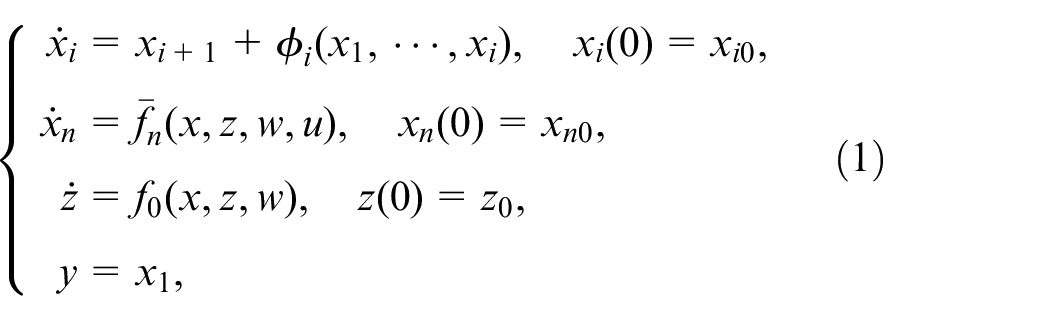
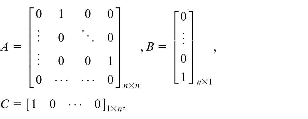
Consider a class of uncertain nonaffine systems:
where ,
system states,
states of internal dynamics,
control input,
measured output,
external disturbances,
mismatched system dynamics,
matched system dynamics,
internal system dynamics,
and contain their respective origins.
The following reasonable assumptions are made for the system (1).
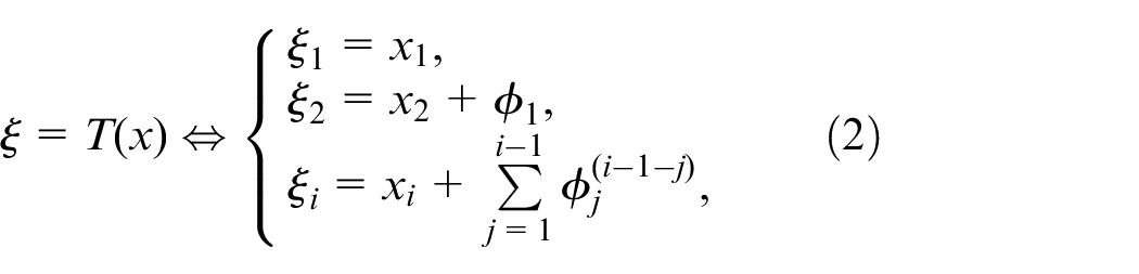
Assumption 1. The mismatched system dynamics , are at least -th order continuously differentiable and locally Lipschitz in their arguments. can be written as , where denotes known system dynamics, is unknown and locally Lipschitz in their arguments. In addition, , .
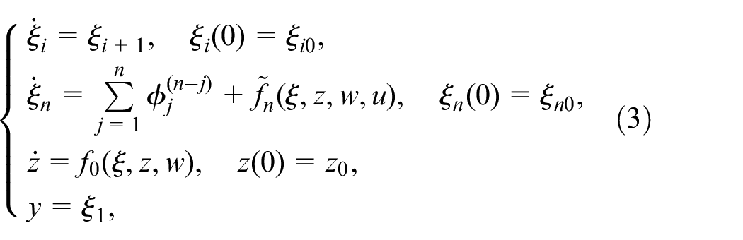
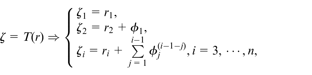
According to Assumption 1, there exists a diffeomorphism10,25
where . The system (1) can be reformulated as:
where and there exists a subset such that .
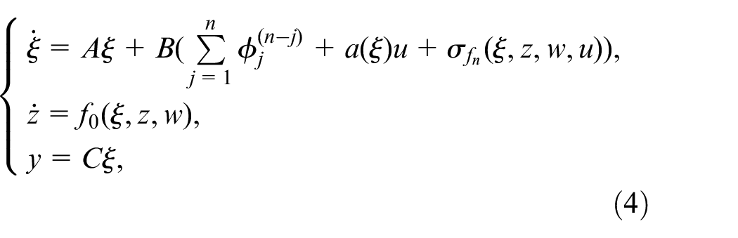
Assumption 2.The function is nozero with known sign and satisfies , where and are positive constants.
Remark 1. Assumption 2 is a common assumption16,20–23,26 and it is a sufficient global controllability condition for the system (3). In other words, Assumption 2 is a sector condition, that is, belongs to the sector , uniformly in its arguments.
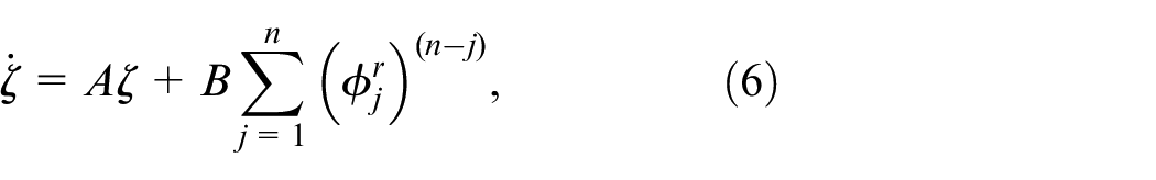
Based on Assumption 2, the system (3) can be rewritten as:
where
and is an auxiliary control input gain, the sign of equals to that of and . It can be shown that by constructing an auxiliary affine control term, the nonaffine system is transformed to an affine system.
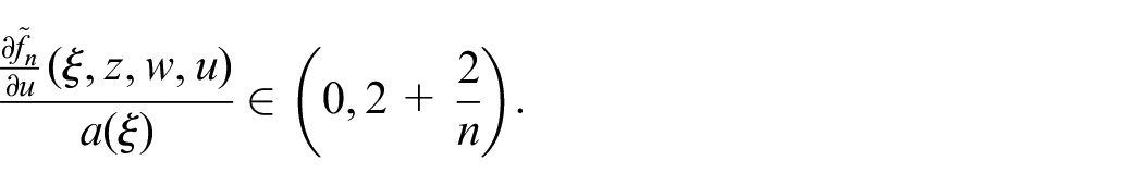
Assumption 3. The auxiliary control input gain satisfies
Remark 2. Assumption 3 is similar to the assumption (A4),8,9 in which performance recovery for uncertain affine systems is achieved by ADRC. It seems like that can be viewed as the equivalent control input gain when a nonaffine systems is viewed as an affine system, and the ADRC design for a nonaffine system is similar to that for an affine system.
Remark 3. Assumption 3 can be always satisfied by appropriate choice of if the upper bound on is known. Taking ensures that Assumption 3 is satisfied. If the upper bound is unknown, one might theoretically end up with a conservative value of . In addition, if is slow time-varying, we can use adaptive mechanism to estimate it online. Otherwise, we have to model it before control design.
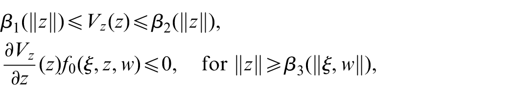
Assumption 4.There exists a positive definite function such that for all
where , and are class functions.
Remark 4 Assumption 4 shows the bounded-input-bounded-state (BIBO) stability of the -subsystem and if can converge into a compact subset in a finite time, the states of the internal dynamics will be bounded. Thus, we will focus on the trajectory of .
Assumption 5External disturbances belongs to a known compact subset , and its time derivative is bounded.
The goal of this paper is to design a robust controller to make the states of system (1) follow those of a target system and the tracking errors are uniformly bounded for all .
Two-time-scale ADRC design
In this paper, we consider two cases, whether the mismatched system dynamics are available or not.
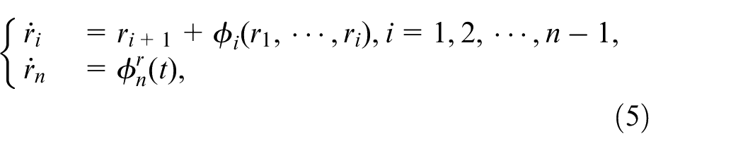
First, we assume that are available. A target system is defined as:
where , is a bounded ideal input.
According to Assumption 1, there exists the same diffeomorphism as that in (2)
and there exists a subset such that . And the target system (5) can be reformulated as:
where .
Define the tracking error as . Its dynamics can be derived as
where .
Assumption 6. There exists a unique continuously differentiable function such that satisfies .
Remark 5. Although it is difficult to find the explicit inversion of nonaffine functions, the existence of such nonlinear function inversion can be guaranteed by the implicit function theorem.
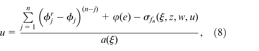
If and are known, we can design the control law as
and the closed-loop system can be derived as
Assumption 7. The state error feedback control satisfies:
is locally Lipschitz in its argument over the domain of interest, and .
is globally bounded function of .
The origin is an asymptotically stable equilibrium point of the closed-loop system with a region of attraction .
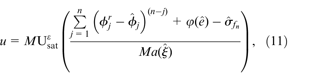
Remark 6 A simple method to design is to select such that is Hurwitz. The global boundedness requirement can be satisfied by saturation of as the equation (11) shows. Since the origin is asymptotically stable and based on Assumption 4, -subsystem is stable.
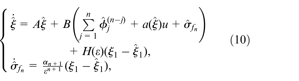
In output feedback where only is available and is unknown, in order to achieve the state feedback control law (8), we design an ESO to estimate and as follows:
where , and the parameters are chosen such that is Hurwitz and is a small positive number.
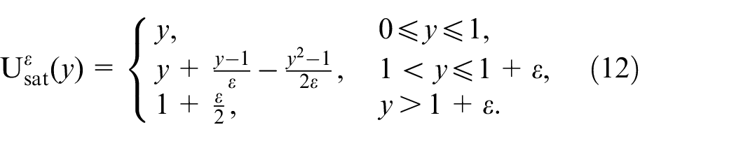
Combining the ESO in (10) with the state feedback control in (8), the output feedback control is designed as:
where , the saturation function is designed to protect the system from peaking phenomenon in the ESO’s transient process and is an odd function which can be expressed as
The saturation bound depends on the compact set of , and we may choose it as a conservative value by trial and error.
Main results
Performance recovery can be seen as a particular kind of state tracking, that is the controlled system has the ability to recover the time responses of the predesigned nominal system. Its definition and the definition of weak performance recovery can be found in the relevant literature.23
It will be proved that in the presence of uncertainties, performance recovery of the original system (1) and integrator-chain system (3) can be achieved, that is, the output feedback control (10) and (11) can drive the original system (1) (respectively, integrator-cascaded system (3)) to follow the target system (5) (respectively, the transformed system (6)).
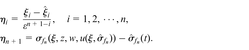
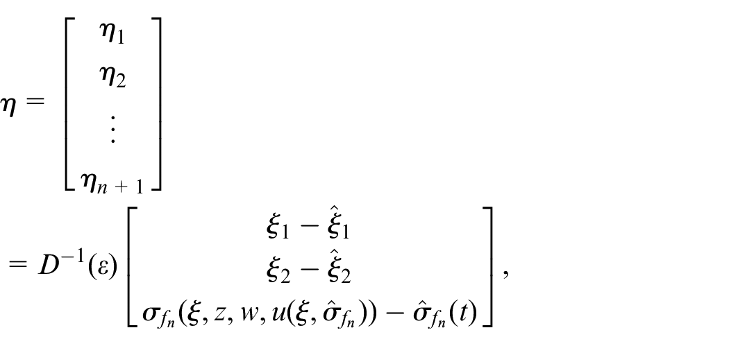
Let the scaled estimation error
Then we have
where
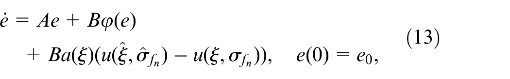
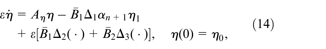
The closed-loop system can be derived as:
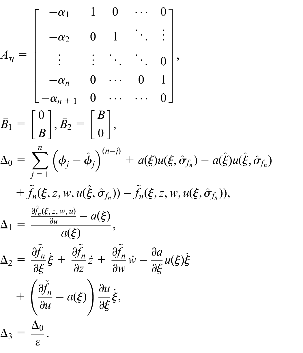
where
Suppose there exist compact subsets in the interior of the region of attraction and in , respectively, such that and .
The closed-loop system (13–14) is a standard singularly perturbed one, and is the unique solution of (14) when . By substituting in (13), the reduced system is nothing but the closed-loop system under state feedback (9)
The boundary-layer system when setting is given by
where .
Theorem 1. Performance Recovery.If Assumptions 1–7 hold, then
1. There exists such that, for every , the trajectory of the system (13–14), starting in , are bounded for all .
2. Given any , there exists and such that, for every , we have
3. Given any , there exists and such that, for every , we have
Proof. The boundedness of the trajectories can be proved in two steps. First, we prove the positive invariance of an appropriately chosen set , which is arbitrarily small in the direction of the scaled estimation error . Second, we prove that any closed-loop trajectory, starting in the compact subset , enters the positively invariant set in finite time.
We know that since the origin of (15) is asymptotically stable with a region of attraction , the converse Lyapunov theorem assures the existence of a Lyapunov function and three positive definite functions , and , all defined and continuous on , such that
for all . The property of in guarantees that with any finite , the set is a compact subset of and is in the interior of .
Lemma 1.If Assumption 3 hold, then there exists a constant matrix and a constant such tha9
For the boundary layer system, we define Lyapunov function which satisfies
Let . Due to Assumptions 1, 4 and 5, we have, for all
where and are positive constants independent of . Moreover, for any , there is independent of , such that, for all and every , we have
In the rest of the proof we always consider . We start by showing that there exist positive constants and (dependent on ) such that the compact set is positively invariant for every . This can be done by verifying that
for all , and
for all , where , is an upper bound for over , . Taking , , where , for every , we have
for all , and
for all . From (23) and (24), we conclude that the set is positively invariant.
Consider . Based on the definition of , there exists a nonnegative number such that . Using (21) and the fact that is in the interior of , it can be shown that
as long as . Thus, there exists a finite time , independent of , such that for all . During this time interval we have
then we deduce
where
To estimate the time that enters into , let
By L’hopital’s rule, we have
Therefore, there exists a small positive number , for every , . Taking guarantees that for every , the trajectory of the closed-loop system enters during and remains there for all . This completes the proof of the first conclusion.
Based on the first conclusion, we can find such that for every , we have
For all , we have
where . Thus, we conclude that
Since is positive definite and continuous, the set is a compact set for sufficiently small . Let and is nondecreasing and . We have . Choosing small enough ensures that is compact and the set is in the interior of , and
For but , we have
where . Then, if , there exists a finite time , for every , we have
Taking and , then (17) follows from (25) and (26). Meanwhile, we conclude that the set is positively invariant, and any trajectory of the closed-loop system starting in enters into in finite time. This completes the proof of the second conclusion.
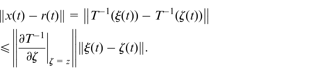
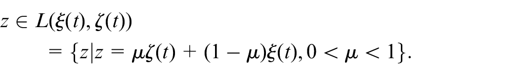
Based on the mean-value theorem, we have
where
Given the property of the diffeomorphism in (2), there exists a constant satisfying
Taking and based on the second conclusion, there exists and such that, for every
Using (27) and (28), we have
This completes the proof of the third conclusion.
Last but not least, let us consider the case that the mismatched system dynamics are unknown, the target system is described as
where , is a bounded command input.
Define the tracking error as , and we can arrive at the following corollary on weak performance recovery with output tracking property.
Corollary 1. Weak Performance Recovery. If Assumptions 1–7 hold, then
There exists such that, for every , the trajectory of the closed-loop system are bounded for all .
Given any , there exist and such that, for every , we have
Given any , there exist , , and such that, for every , we have
Remark 7. The weak performance recovery stated in Corollary 1 has output tracking property compared with the IDI method,23 which suggests better feasibility from the perspective of engineering.
Proof. The proof of the first and second conclusions in Corollary 1 is similar to those in Theorem 1, we neglect it here. In what follows, we will prove the third conclusion in Corollary 1.
Based on the second conclusion in Corollary 1, for any , and such that, for every , we have
Since and by using (29), there exist positive constants and such that
where
Experiments: Magnetic levitation ball system
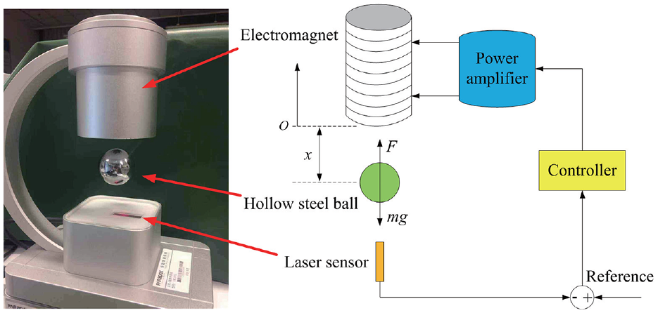
Magnetic levitation ball system is a typical example of a practical nonaffine system, which is shown in Figure 1. The magnetic levitation ball system is composed of an electromagnet, a hollow steel ball, a laser sensor, a power amplifier and a controller. The laser sensor measures the position of the hollow steel ball, and the controller sends control signal to the power amplifier based on the position error. The power amplifier regulates current of the electromagnet to make the steel ball to remain in a given position or to track a desired trajectory.
The diagram of the principle of magnetic levitation ball system.
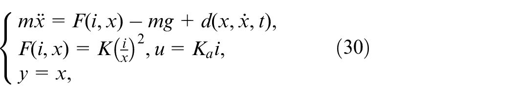
The mathematical model of the magnetic levitation ball system can be described as follows
where
position of the steel ball,
mass of the steel ball,
instantaneous current of electromagnetic coil,
mutual inductance of electromagnetic coil,
acceleration due to gravity,
gain of the power amplifier,
controlled voltage,
measured output,
external disturbances.
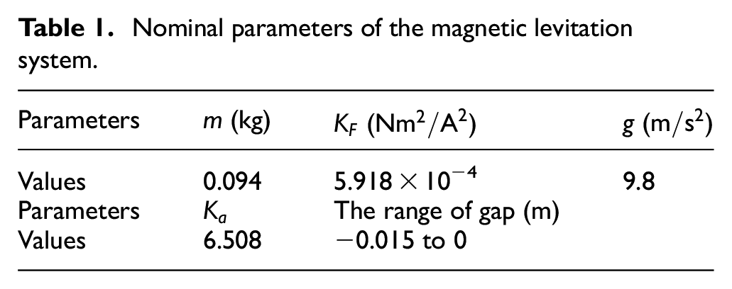
Nominal parameters of the system are given in Table 1.
Nominal parameters of the magnetic levitation system.
Parameters
(kg)
()
()
Values
0.094
5.918 × 10⁻⁴
9.8
Parameters
The range of gap (m)
Values
6.508
−0.015 to 0
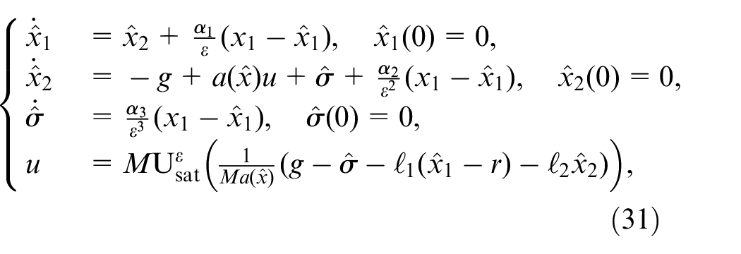
For the magnetic levitation ball system (30), the proposed ADRC can be designed as
where is the auxiliary control gain, represents the total disturbances, including model uncertainties and external disturbances. And , and are the estimates of , and , respectively.
To show the superiority of the proposed ADRC scheme in (31), another two control methods, that is, the existing linearization-based ADRC method27 and the ADI-based method,28 are introduced. The specific design process can be referred to the paper,28 so it is omitted here due to page limits.
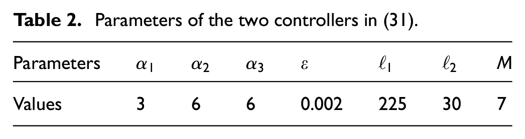
Control parameters of the proposed ADRC in (31) are given in Table 2. The procedure for configuring control parameters of the proposed ADRC (31) can be described as follows:
In simulations, control gains and are chosen to meet design criteria under the state feedback. The saturation bound in (31) is chosen such that the saturation is not activated under the state feedback.
For the designed ESO in (31), a common method to choose parameters is to guarantee that is Hurwitz. By trial and error, is chosen to guarantee the stability and performance requirements of the closed-loop system.
In experiments, we need to make trade-off among performance, noise-sensitivity, time-delay and other factors and may retune the parameters based on the well-tuned parameters in simulations.
Parameters of the two controllers in (31).
Parameters
Values
3
6
6
0.002
225
30
7
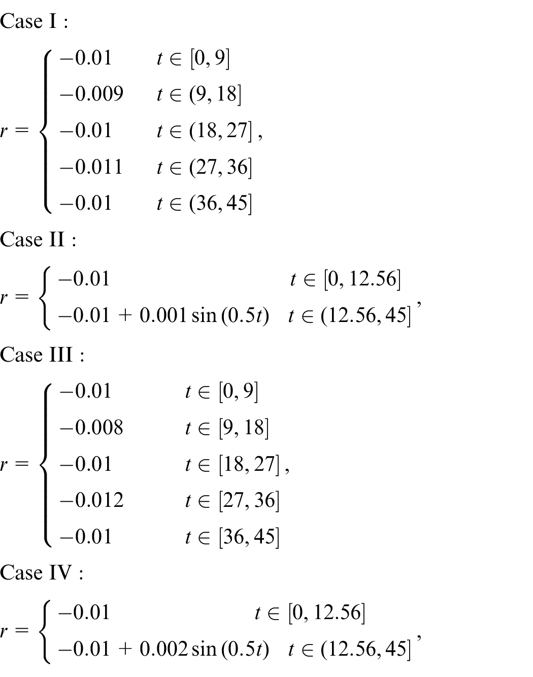
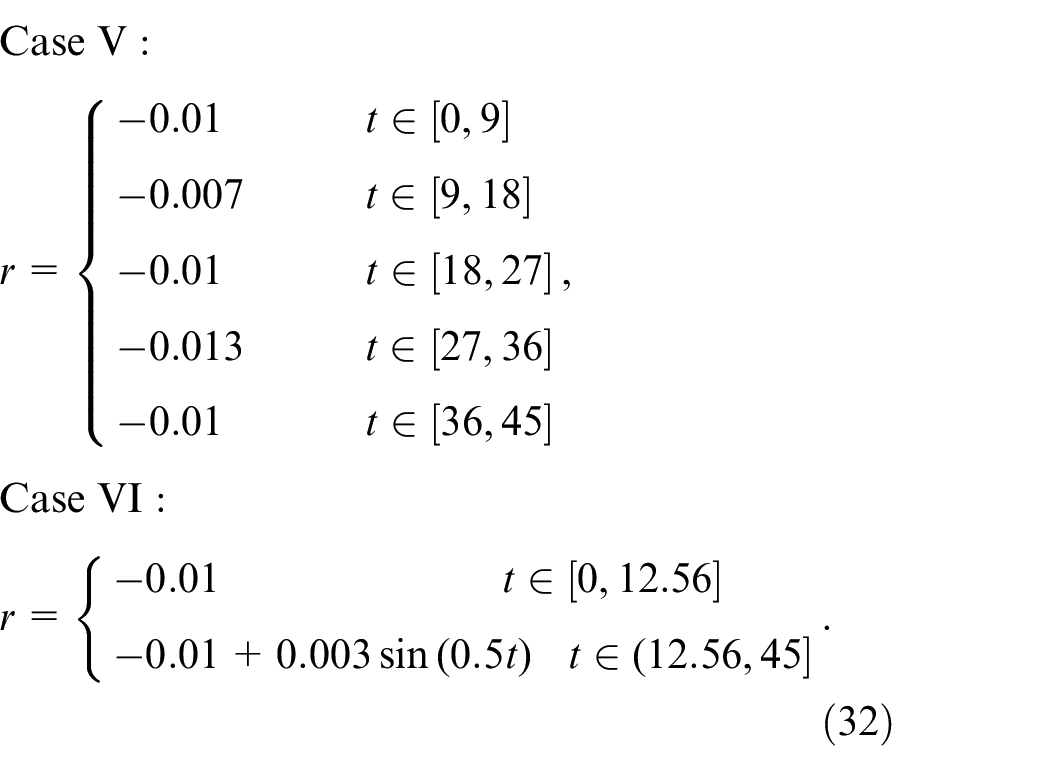
In the experiment, the sampling time is set to be 0.001 s and the solver is set to be ode 1 (Euler) in the MATLAB/Simulink environment. Regulation and tracking problems are considered and six cases of reference signal are expressed as
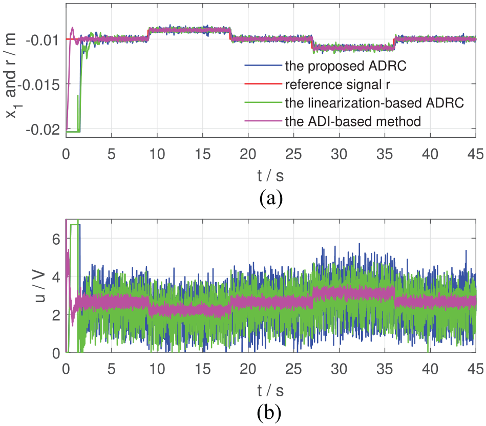
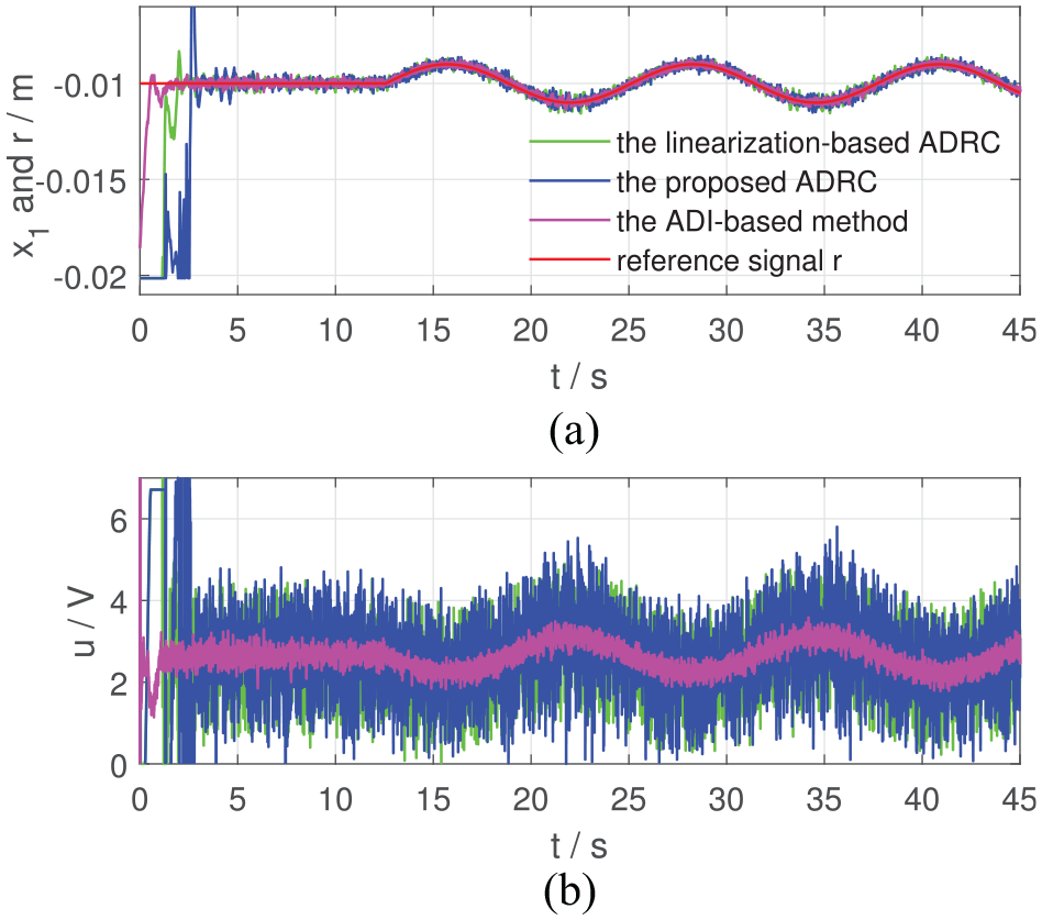
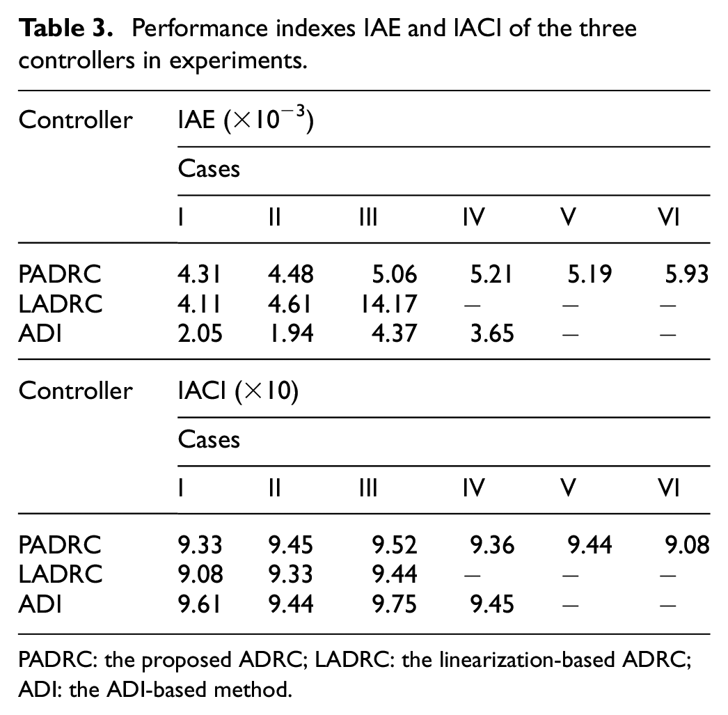
In Cases I–VI, the motion ranges of the steel ball becomes larger with more system uncertainties. Responses and control signals of the proposed ADRC, the linearization-based ADRC and the ADI-based method for the reference signals in (32) are shown in Figures 2 to 7. To evaluate the system performance quantitatively, two indexes, integral of absolute error (IAE), integral of absolute control input (IACI), are introduced and listed in Table 3.
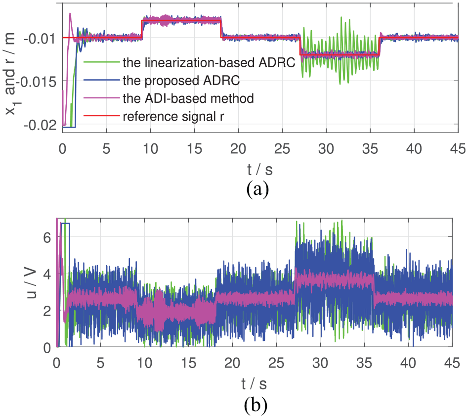
Regulation performance of the two controllers in Case I: (a) and the reference signal and (b) control inputs.
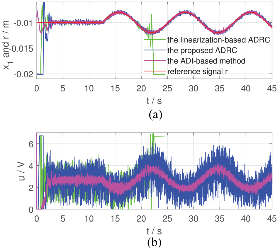
Tracking performance of the two controllers in Case II: (a) and the reference signal and (b) control inputs.
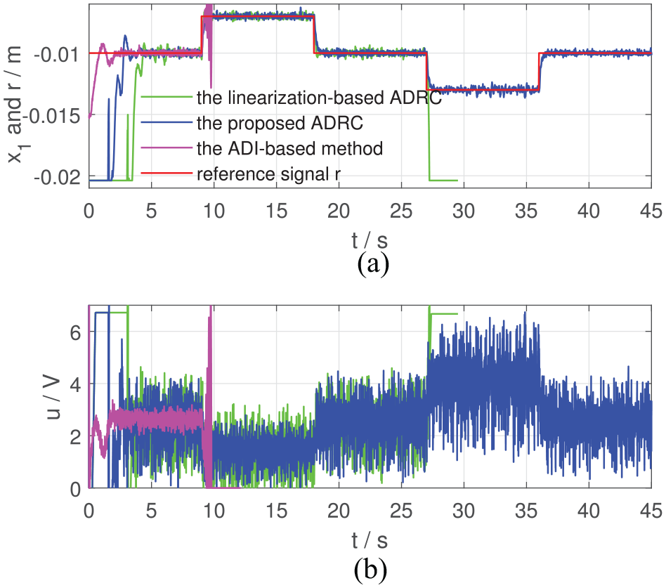
Regulation performance of the two controllers in Case III: (a) and the reference signal and (b) control inputs.
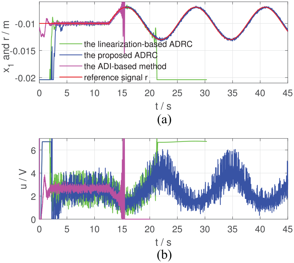
Tracking performance of the two controllers in Case IV: (a) and the reference signal and (b) control inputs.
Regulation performance of the two controllers in Case V: (a) and the reference signal and (b) control inputs.
Tracking performance of the two controllers in Case VI: (a) and the reference signal and (b) control inputs.
Performance indexes IAE and IACI of the three controllers in experiments.
Controller
IAE (×10−3)
Cases
I
II
III
IV
V
VI
PADRC
4.31
4.48
5.06
5.21
5.19
5.93
LADRC
4.11
4.61
14.17
−
−
−
ADI
2.05
1.94
4.37
3.65
−
−
Controller
IACI (×10)
Cases
I
II
III
IV
V
VI
PADRC
9.33
9.45
9.52
9.36
9.44
9.08
LADRC
9.08
9.33
9.44
−
−
−
ADI
9.61
9.44
9.75
9.45
−
−
PADRC: the proposed ADRC; LADRC: the linearization-based ADRC; ADI: the ADI-based method.
From Figures 2 to 7, the proposed ADRC can regulate at the given position in Cases I, III and V and make track the desired trajectory in Cases II, IV and VI. In Case I and Case II where the required motion range is just 0.001 m, the linearization-based ADRC can achieve the control objective. However, when the desired motion range becomes larger, the performance of the linearization-based ADRC evolves worse. In Figure 4, from 27 to 36 s when m, the trajectory of the linearization-based ADRC oscillates around m with an amplitude of 0.004 m, which shows bad regulation performance (IAE = 14.17, much larger than those in Case I and Case II, according to Table 3). In Figure 6, cannot be regulated at m at 27 s by the linearization-based ADRC and drops at m, that is, the steel ball drops to the bottom of the magnetic levitation device. From Figures 5 and 7, at about 20.2 s, the trajectories of of the linearization-based ADRC begin to oscillate and finally drops to m.
As for the ADI-based method, from Case I to Case IV, the ADI-based method can achieve the control objective. One detail to be noticed is that in Case III, from 9 to 18 s when m, the trajectory of the ADI-based method oscillates around m with an amplitude of 0.001 m and the control effort varies with an amplitude of 2 V. In Case V and Case VI, at about 9 and 14 s, the trajectories of of the ADI-based method begin to oscillate and then blow up. Finally, after about 1 s, the control effort drops to 0, and the control tasks fail.
The most obvious advantages of the ADI-based method are the smoothness of the control inputs shown in Figures 2 to 5, which is brought by the low-pass filter property of the ADI block, and high tracking precision shown in Table 3. Meanwhile, since the closed-loop system has a three timescale structure, in which the ADI block has to occupy the intermediate timescale, time-delay of the ADI block has adverse effects on the system performance, including response rate and robustness. Therefore, the proposed two timescale ADRC performs better than the ADI-based method in Case V and Case VI.
The main reason why the proposed ADRC performs better than the linearization-based ADRC is that we apply the state-dependent control gain rather than the constant control gain. Thus, the proposed ADRC can be viewed as a kind of variable-gain nonlinear control method.
To sum up, experimental results of Figures 2 to 7 and Table 3 show that the proposed ADRC is more robust to the system uncertainties than the linearization-based ADRC and the ADI-based method and demonstrate the effectiveness of the proposed ADRC scheme.
Simulations: Nonlinear ship autopilot
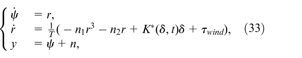
We consider a physical system of nonlinear ship autopilot to illustrate the proposed control method. A ship autopilot with nonlinear damping can be described as a nonaffine system29
where
yaw angle,
yaw angular velocity,
time constant,
nonlinear damping coefficients,
equivalent control input gain,
rudder angle (control input),
wind moment,
measured output,
measurement noises.
Remark 8. The equivalent control input gain is related to the control input . Even we know accurately and design the moment , it may be difficult to derive the control input .
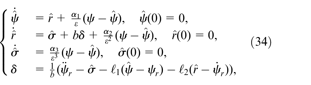
The control goal is to design to make the system output follow a desired signal with and being its first time derivative and second time derivative, respectively. The desired signal is . Some parameters are set as with being the sign function. Saturation of the rudder angle is . The initial values are . To achieve the control objective, the proposed ADRC can be designed as
where the auxiliary control input gain . Variables , and are estimates of , and system uncertainties, respectively.
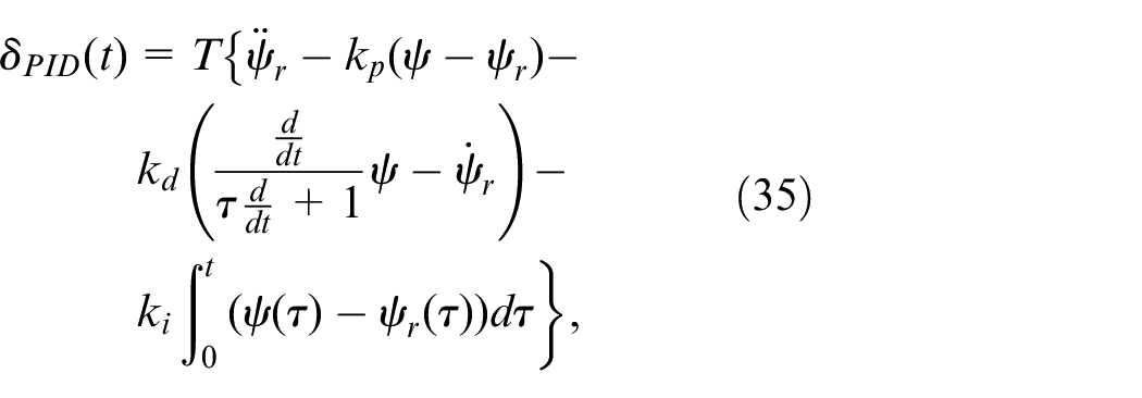
A dirty derivative-based proportional-integral-derivative (PID) controller is introduced and can be designed as
where and are the proportional, derivative and integral gains, respectively. is the time constant of the first-order low pass filter.
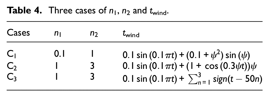
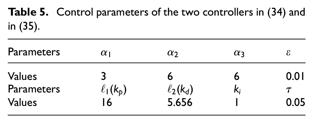
In simulations, the sampling time is set to be 0.01 s and the solver is set to be ode 4 (Runge-Kutta) in the MATLAB/Simulink environment. Three cases of and are tested and listed in Table 4, where is the nominal case. The control parameters of the proposed ADRC (34) and the dirty derivative-based PID (35) are tuned to achieve similar performance to guarantee fairness, which are shown in Table 5. Simulation results are shown in Figure 8. To evaluate the system performance quantitatively, two indexes, including IAE and IACI, are introduced and listed in Table 6.
Three cases of n1, n2 and twind.
Cases
twind
0.1
1
1
3
1
3
Control parameters of the two controllers in (34) and in (35).
Parameters
Values
3
6
6
0.01
Parameters
Values
16
5.656
1
0.05
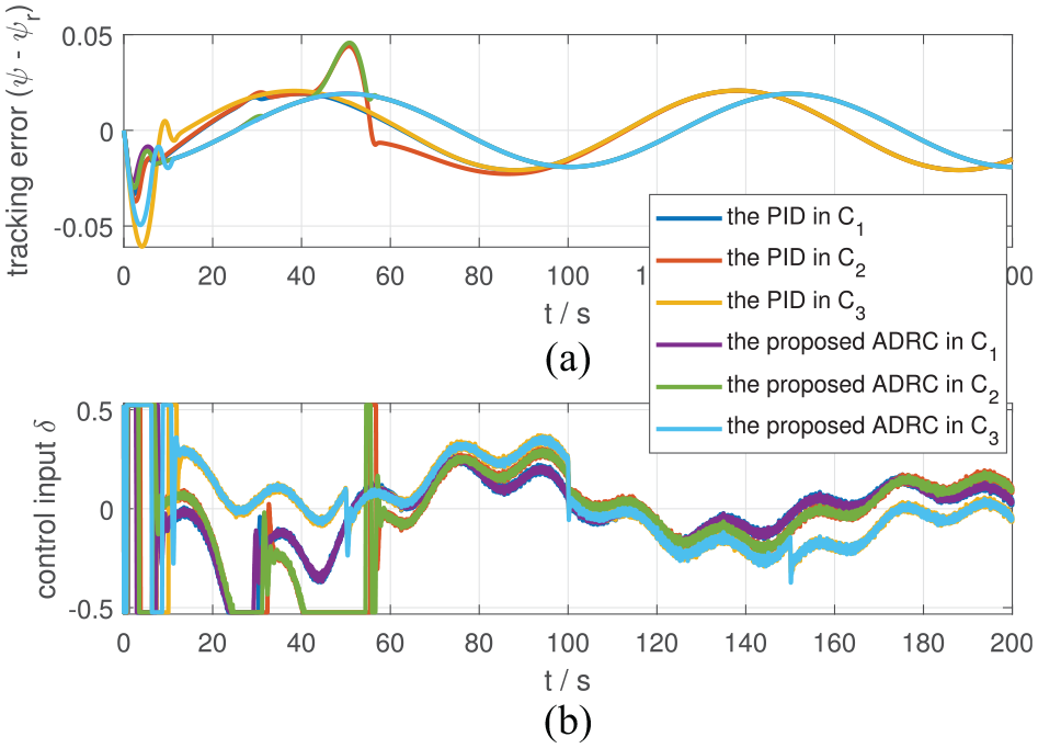
Tracking performance of the two controllers in (34) and in (35): (a) tracking errors and (b) control inputs .
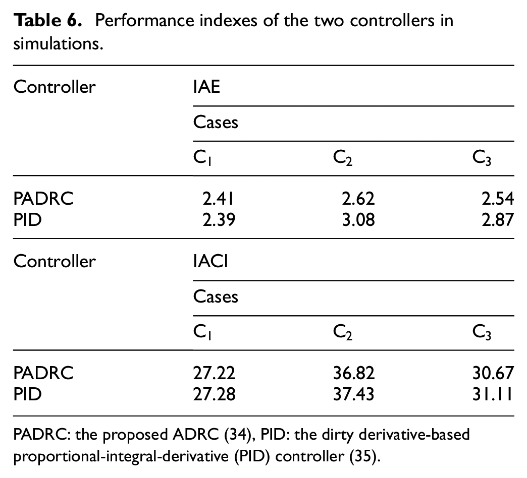
Performance indexes of the two controllers in simulations.
Controller
IAE
Cases
PADRC
2.41
2.62
2.54
PID
2.39
3.08
2.87
Controller
IACI
Cases
PADRC
27.22
36.82
30.67
PID
27.28
37.43
31.11
PADRC: the proposed ADRC (34), PID: the dirty derivative-based proportional-integral-derivative (PID) controller (35).
From Figure 8, in the nominal case , the proposed ADRC and the PID have similar transient process and steady state errors (about 0.02). However, as the system uncertainties become larger shown in and , the proposed ADRC (34) performs better than the PID controller (35). The maximum tracking error of the PID reaches to 0.06, while that of the proposed ADRC is only 0.042. Meanwhile, based on Table 6, both IAE and IACI indexes of the proposed ADRC are smaller than those of the PID, which shows the superiority of the proposed control scheme.
One thing to be noticed based on large amount of simulations we have done is that it is almost impossible to apply the IDI method and the ADI-based methods to the ship autopilot task to achieve the control objective in the above simulation environment due to the limited system bandwidth and control input saturation.
Conclusions
This paper investigates performance recovery of a class of uncertain nonaffine systems and a systematic two-time-scale ADRC scheme is proposed. We transform the strict-feedback nonaffine system into an integrator-chain nonaffine system with a diffeomorphism. By constructing an auxiliary control input term, the integrator-chain nonaffine system is transferred to an affine one. Then, a two-time-scale ADRC scheme is proposed. Under some mild assumptions, it can be proved that the proposed ADRC-based closed-loop system can achieve performance recovery and weak performance recovery in different cases of mismatched system dynamics, respectively. Experimental results of the magnetic levitation ball system verify the effectiveness of the proposed ADRC design.
As indicated in Remark 3, if the upper bound of is unknown, we have to choose big enough, which lead to larger system uncertainties. So the parameter in the designed ESO (10) has to be tuned small enough to guarantee the stability of the overall system. However, in practical applications, due to ubiquitous noises, unavoidable time-delay and limited sampling rate, cannot be tuned arbitrarily small. So the system stability cannot be ensured, which may lead to dangerous outcomes. Thus, how to choose the auxiliary control input gain to satisfy Assumption 3 is a critical, and may difficult, problem in the practical application of the proposed ADRC. Further research work will explore some effective methods to overcome this limitation and to extend the proposed control scheme to multi-input-multi-output systems and non-minimum phase systems.
Footnotes
Declaration of conflicting interests
The author(s) declared no potential conflicts of interest with respect to the research, authorship, and/or publication of this article.
Funding
The author(s) received no financial support for the research, authorship, and/or publication of this article.
ORCID iD
Zhixiang Chen
References
1.
AstromKJKumarP.Control: a perspective. Automatica2014; 50(1): 3–43.
FengHGuoB.Active disturbance rejection control: old and new results. Annu Rev Control2017; 44: 238–248.
4.
GaoZ. Active disturbance rejection control: from an enduring idea to an emerging technology. In: International workshop on robot motion and control, Poznan, Poland, 6–8 July, pp. 269–282. New York, NY: IEEE.
5.
ZhengQPingZSoaresS, et al. An optimized active disturbance rejection approach to fan control in server. Control Eng Pract2018; 79: 154–169.
6.
YuanYChengLWangZD, et al. Position tracking and attitude control for quadrotors via active disturbance rejection control method. Sci China Inf Sci2019; 62(1): 010201.
7.
XueWZhangXSunL, et al. Extended state filter based disturbance and uncertainty mitigation for nonlinear uncertain systems with application to fuel cell temperature control. IEEE Trans Ind Electron2020; 67(12): 10682–10692.
8.
XueWHuangY.Performance analysis of 2-DOF tracking control for a class of nonlinear uncertain systems with discontinuous disturbances. Int J Robust Nonlinear Control2018; 28(4): 1456–1473.
9.
XueWHuangY.Performance analysis of active disturbance rejection tracking control for a class of uncertain LTI systems. ISA Trans2015; 58: 133–154.
10.
ZhaoZLGuoBZ.A novel extended state observer for output tracking of MIMO systems with mismatched uncertainty. IEEE Trans Automat Control2018; 63(1): 211–218.
11.
ChenSChenZXZhaoZL, et al. New design of active disturbance rejection control for nonlinear uncertain systems with unknown control input gain. Sci China Inf Sci2022; 65(4): 142201–142215.
12.
ZhangTGuayM.Adaptive control of uncertain continuously stirred tank reactors with unknown actuator nonlinearities. ISA Trans2005; 44(1): 55–68.
13.
BianTJiangYJiangZ P.Adaptive dynamic programming and optimal control of nonlinear nonaffine systems. Automatica2014; 50(10): 2624–2632.
14.
BoskovicJDChenLMehraRK.Adaptive control design for nonaffine models arising in flight control. J Guid Control Dyn2004; 27(2): 209–217.
15.
BoulkrouneAM’SaadMFarzaM.Fuzzy approximation-based indirect adaptive controller for multi-input multi-output non-affine systems with unknown control direction. IET Control Theory Appl2012; 6(17): 2619–2629.
16.
LavretskyEHovakimyanN. Adaptive dynamic inversion for nonaffine-in-control uncertain systems via time-scale separation. Part II. J Dyn Control Syst2008; 14(1): 33–41.
17.
GeSSZhangJ.Neural-network control of nonaffine nonlinear system with zero dynamics by state and output feedback. IEEE Trans Neural Netw2003; 14: 900–918.
18.
LiuYTongS.Adaptive nn tracking control of uncertain nonlinear discrete-time systems with nonaffine dead-zone input. IEEE Trans Cybern2015; 45(3): 497–505.
19.
FallahHAliGKalatA.Observer-based hybrid adaptive fuzzy control for affine and nonaffine uncertain nonlinear systems. Neural Comput Appl2016; 30: 17–32.
20.
MolaviAJalaliANaraghiMG.Adaptive fuzzy control of a class of nonaffine nonlinear system with input saturation based on passivity theorem. ISA Trans2017; 69: 202–213.
21.
LeeJMukherjeeRKhalilH K.Output feedback performance recovery in the presence of uncertainties. Syst Control Lett2016; 90: 31–37.
22.
RanMWangQDongC.Active disturbance rejection control for uncertain nonaffine-in-control nonlinear systems. IEEE Trans Automat Control2017; 62(11): 5830–5836.
23.
YiBLinSYangB, et al. Performance recovery of a class of uncertain non-affine systems with unmodelled dynamics: an indirect dynamic inversion method. Int J Control2018; 91(2): 266–284.
24.
ChenZGaoQChenS, et al. Linear active disturbance rejection control for nonaffine strict-feedback nonlinear systems. IEEE Access2019; 7: 120030–120040.
25.
GuoBZWuZH.Output tracking for a class of nonlinear systems with mismatched uncertainties by active disturbance rejection control. Syst Control Lett2017; 100: 21–31.
26.
GeSSHangCCZhangT.Adaptive neural network control of nonlinear systems by state and output feedback. IEEE Trans Syst Man Cybern B: Cybern1999; 29(6): 818–828.
27.
WeiWXueWLiD.On disturbance rejection in magnetic levitation. Control Eng Pract2019; 82: 24–35.
28.
ChenZGaoQ.Active disturbance rejection controller for uncertain nonaffine systems by dynamic inversion. Control Theory Appl2020; 37(11): 2365–2382.
29.
FossenTI. Handbook of marine craft hydrodynamics and motion control. New York, NY: John Wiley & Sons.