Sage Journals: Discover world-class research

Abstract

Presently, mobile robots experience problems of time consumption, poor security, and high computational complexity in global path-smoothing algorithms. This study presents a multiobjective path-smoothing algorithm, including a path point adjustment algorithm and a turn-smoothing method called the point adjustment algorithm and smoothing. First, the proposed path point adjustment algorithm filters and moves the nodes in an original path to decrease the length of the path and increase the angle of the turns in the path. Second, the proposed turn-smoothing method inserts the B-spline curve into the processed path to smooth the discontinuous turns in the path. Subsequently, the positions of the control points are adjusted based on the property of the B-spline to ensure that the smoothed path can avoid obstacles and satisfy the maximum curvature constraint. Simulation results show that the proposed algorithm can quickly calculate the path satisfying the robot dynamic constraints in various environments combined with different global path planning algorithms. Compared with other mainstream path-smoothing algorithms, this algorithm makes a substantial improvement in path length.

Keywords

Path smoothing node adjustment path simplification trajectory optimisation B-spline curve

Introduction

Generally, the path planning algorithm involves the technology that provides a barrier-free path for a mobile robot through the initial place and the target place. Combined with the trajectory planner method^1–3 that controls a mobile robot to travel along the path, this technology can liberate robots from a fixed working position to complete more complex tasks and can improve the repeatability of robotic applications, which greatly enhances the robots’ application scenarios.^4–7 Recently, this has been a trending research topic in robotics.

For plane path planning problems, researchers worldwide have introduced many classic algorithms, which can be roughly divided into searching-based planning methods,^8–10 sampling-based planning methods,^11,12 and artificial potential field methods,¹³ according to their principles. The path planning problem scenarios in the 3D environment are more complex, the path degree of freedom is higher, and the path optimization needs to consider more constraints, which has attracted more and more researchers’ attention in recent years.^14,15 However, the path obtained by these algorithms is often polygonal lines, which are composed of line segments. When the robot travels along this path, it will have to stop moving at the corners to make a turn, increasing the traveling time. Moreover, the sudden change in curvature occurring at these corners destabilizes the control system and causes machine wear. This paper focuses on path smoothing methods, which are an integral part of mobile robotics. Considering the dynamic requirements of robot movement, this paper proposes a path smoothing method based on the geometric method to improve the path performance in terms of length, smoothness and other indicators.

To improve the path quality, in 1957, Dubins¹⁶ proposed a method that uses a circle arc and line elements to generate a smooth path connecting the start and goal points of a robot in a two-dimensional (2D) plane. Considering the vehicle’s forward and backward function, Reeds and Sheep¹⁷ improved this algorithm in 1990. Later, scholars designed many path-smoothing methods based on different curves, such as Bezier,¹⁸ B-spline,^19,20 and clothoids.²¹ However, these methods have yet to attain a good balance between path quality and solution efficiency. As the application range of robots has become more extensive recently, the requirements for moving paths have increased. Especially for the UAV path planning problem in the 3D environment, higher requirements are put forward.²² Therefore, many planning algorithms for the path smoothness problem have been proposed. These algorithms can generally be divided into two categories.²³ Some algorithms add the path smoothing module on the basis of typical geometric path planning methods (e.g., RRT, A*) to solve the path smoothness problem step-by-step. Other algorithms add time information to the path and use numerical optimization or other methods to directly solve a path that satisfies the constraints. This problem-solving method is also known as the trajectory planning algorithm. Both methods can improve the quality of the path. The method combined with the geometric path planning method usually uses information, such as mathematical methods and path characteristics to improve the efficiency of the solution, but the generality is not good. The trajectory planning method can directly find a path that meets the requirements but is not very efficient. This paper mainly focuses on smoothing methods combined with typical geometric methods, which can be divided into two parts: geometric^24–30 and optimisation^31–36 methods.

Fnadi et al.²⁴ designed a local path-smoothing method using cubic Bezier curves. By inserting control points near obstacles, Bezier curves are generated by these control points to meet the requirements of obstacle avoidance and path smoothness. However, this method is only useful for avoiding the obstacles represented by circles. Similarly, Elmokadem²⁵ used the deformation method to adjust the Bezier curve to avoid obstacles in a local environment. This method can smoothly avoid obstacles of any shape without obtaining map information in advance. However, using this type of insertion algorithm, a sudden change in curvature may occur at the path turning point. Furthermore, some scholars use the turning strategy for local path smoothing. In a previous study,²⁶ the corner points of the path are diffused until they attain a certain distance from the obstacles. The cycloid curves are constructed according to the angles between these diffusion points. Next, the cycloid curves are rotated to a collision-free position to complete a local smooth turning task. A steering problem of automobiles on a real road was simulated in a previous study.²⁷ The authors rotated the arcs constructed by turning the radius to avoid and turn obstacles. Next, the paths between corners were smoothened using the Bezier curve. For the convex hull property of the Bezier curve, the method ensures that the path does not collide. Choi et al.²⁸ proposed two path-smoothing methods based on the Bezier curve. By adding constraints to the Bezier curve at the turns, each slope of the curve at the corner is tangent to the trajectory, and the first- and second-order derivatives of the curve are both minimized using the optimization method so that the robot’s angular acceleration changes smoothly while turning. Similar to the first method, the solution is simplified by constructing the left-right symmetry at the turning point in the second plan, which speeds up the solution process. However, the results in the generated trajectory offset the original path more. In addition, the methods do not consider the problem of obstacle avoidance. Caldeira et al.²⁹ uses the Bezier curve to solve the obstacle avoidance problem in three-dimensional space, and limits the maximum speed of the robot movement, but does not consider the smoothness of the movement route.

The path-smoothing algorithm that only acts on a local environment easily extends the global path considerably. In a previous study,³⁰ a novel RRT algorithm was proposed, which simultaneously combines the path-smoothing and path-planning processes to obtain a smooth path in the global environment. Specifically, this method selects the Bezier curve to connect randomly generated points X_rand with the point X_near closest to X_rand in the search tree when generating RRT. Meanwhile, it uses the smoothed curve to detect whether a collision occurs, and the result is regarded as a condition for terminating the RRT iteration. Simultaneous searching and smoothing can effectively compress the running time, and the probability of finding a feasible solution increases. However, the quality of the obtained path may not be as high as the step-by-step searching and smoothing, and the time-consuming smoothing operation may be performed more than when it is separated.

For the two basic requirements of obstacsle avoidance and smoothing, Luo et al.³¹ used the gradient optimisation method to extend points in the original path further away from obstacles. They also used variable-order Bezier curves to smoothen the filtered path. After optimizing the original path points, the path can be kept away from obstacles, but the subsequent smooth process does not consider the obstacle avoidance problem, and this method substantially extends a planned path. Similarly, Heiden et al.³² used the gradient descent method to move vertices in an original path to farther distant path points from obstacles and insert vertices in the path to make more path points closer to obstacles. Next, they designed a short-cutting technique based on the cost to delete unnecessary path points to simplify the path. On this basis, Wang et al.³³ used the Bellman-Ford method to reconnect and delete the moved path points to obtain the shortest path formed by these path points. This method sets the optimization goal to keep path points away from obstacles. Thus, the obtained path will be greatly improved in terms of safety, and after optimisation processing, the path-smoothing phases will be easier. However, an optimization process is cumbersome and difficult to adjust. In addition, it is difficult to guarantee the final path performance in other aspects. Wang et al.³⁴ added path smoothness to the local path planning method as constraints and added speed information to the path planning method, which can still maintain good results in complex environments.

Additionally, Cimurs and Suh³⁵ combined geometric and optimisation methods. In each line segment, the Bezier curve is redesigned to obtain a shorter path that meets the dynamic requirements (angular velocity requirement) by adjusting the start and end points using an optimization method. However, in this optimization process, the two endpoints P_i and P_i₊₁ must be calculated simultaneously. However, only one optimisation point P_i is determined, and the other object P_i₊₁ must be fixed in the next iteration, which increases the computational time. Yang et al.³⁶ used an ant colony algorithm to filter the original path in the trajectory-smoothing phase to obtain a path with fewer turns. On this basis, the B-spline curve was used to smooth the turns in the path. The path obtained using this method had a high degree of fitting with the original path, but the obstacle avoidance requirement of the path smoothed by the B-spline curves is not considered in this article.

Hence, the above path-smoothing algorithms have the following two deficiencies. First, they only detect collisions for an original path without considering whether the smoothed path will collide. Second, only local area smoothing leads to failure when finding a high-quality path suitable for the overall situation. To solve the above shortcomings, this paper proposes a global path-smoothing algorithm, which increases the fit degree between the smoothed and original paths to improve a path’s global performance and detect collisions for the smoothed path combined control point adjustment to ensure the security of a smoothed path.

The main contributions of this paper are as follows:

A smoothing method for only the discontinuous parts of an original path is proposed, which can reduce obstacle avoidance detection and better retain the characteristics of an original path.

A method for adjusting the path after B-spline smoothing is proposed to meet the path requirements of continuity and collision-free robot movement.

A path point adjustment algorithm is proposed to reduce the path length and make the path easier for a robot to turn and for smoothing operations.

As a general path-smoothing algorithm, this algorithm fits an original path that can be better obtained by arbitrary path planning methods, and compared with other path-smoothing algorithms, the obtained path is better in length and smoothness.

The path-smoothing problem in the grid-based map is defined in Section “Environmental description and problem definition.” The path-processing algorithm performed on an original path is described in Section “A path point adjustment algorithm for increasing angles between path segments.” The B-spline smoothing method that acts on the turns of a path is introduced in Section “B-spline path smoother acting at turns of path.” The smoothing algorithm proposed in this paper is evaluated and compared with other path-smoothing algorithms using a simulation in Section “Experiments.” The conclusion and future work are elaborated on in Section “Conclusion.”

Environmental description and problem definition

Environmental description

Consider the construction of a robot’s moving path in a 2D environment. The robot’s working environment is described as a rasterized 2D space where some known static obstacles are distributed. The robot is regarded as a mass point in space. Considering the influence of a robot’s actual size, obstacles need to be “expanded” in practical applications.

Problem definition

Suppose the start and end positions of the robot are the start and goal, respectively. Finding a curve connecting them in a grid space, {T₀, T₁, T₂, …T_n}, where T₀ and T_n are the start and goal, respectively, means finding the robot movement path.

The above process can be accomplished with path planning algorithms. Considering the dynamic requirements of a robot in actual movement, the path-smoothing phases are usually added after a path planning algorithm so that the designed path can meet more constraints and be more suitable for robot movement. For wheeled robots with nonholonomic constraints, the curvature of the path is related to the turning radius of the robot.³⁷ Therefore, to provide a smooth path and ensure the stability of robot movement, the continuity of curvature in the path is one of the goals that the path smoothing algorithm must achieve. In addition, reducing the maximum curvature value in the path can provide the robot with a larger turning radius so that the turning process can be performed better, which is very important in some overloading and other occasions.³⁸ In summary, based on a previous study by Elbanhawi et al.,³⁹ the goals of our path-smoothing algorithm were set as follows:

(1) The path passes through the start and end positions of the robot’s movement.

(2) The path should be smooth everywhere, satisfying C⁰, C¹, and C² order continuity.

(3) The path does not collide with obstacles distributed in space.

(4) The maximum curvature value in the path is less than the maximum curvature that a robot can achieve when turning.

The whole process

The whole algorithm flow of this paper is shown in Figure 1.

Figure 1.

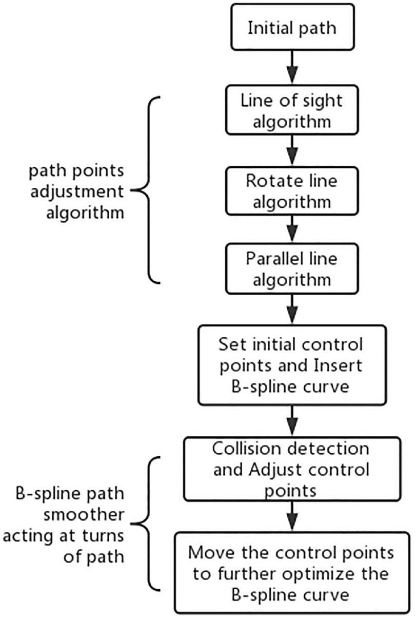
The whole algorithm flow.

A path is initially obtained by classical path planning methods, such as RRT. Then, the obtained path is adjusted by the designed path point adjustment algorithm to increase the angle of the turns in the path and remove redundant turns. Then, the control points are set at the turns of the path to insert B-spline curves into the path and replace the original path segment near turns. Finally, the algorithm further optimizes the B-spline curve through two control point adjustment methods.

A path point adjustment algorithm for increasing angles between path segments

The quality of a smoothed path largely depends on the quality of an original path. A path planning algorithm usually obtains an obstacle-free path that has passed collision detection. Thus, proximity to the original path during the path-smoothing process can greatly reduce obstacle avoidance and improve efficiency. From the B-spline properties, the larger the angles of a path formed by connecting the control points, the better the traceability of B-spline curves to the path. Msohamed Elbanhawi and Simic⁴⁰ proposed a point-trimming method (line of sight algorithm). However, they did not consider the fitness between the smoothed and original paths. Therefore, the path point adjustment algorithm is proposed in this section to process an original path before smoothing to increase the angles in a path and simultaneously reduce the length of an original path.

Line of sight algorithm

Figure 2 shows that the green curve is the path calculated using the RRT algorithm, which can be represented by the path point sequence {T₀, T₁, T₂, …, T_n}. Many unnecessary turns exist in the path. By removing redundant path points, the smoothing process and the length of a path can be reduced.

Figure 2.

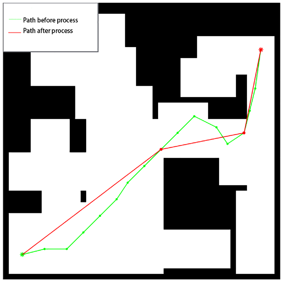
Line of sight algorithm result on path obtained by RRT.

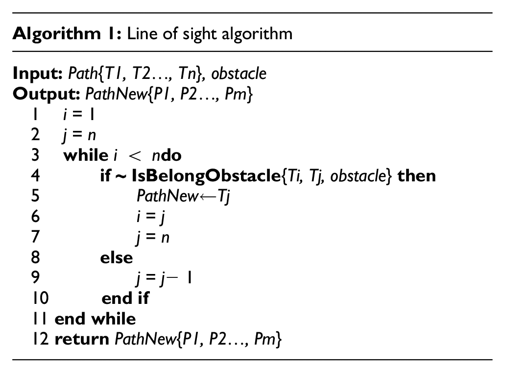
If a point in the path can skip the next point to connect with the back points without collision, then these skipped points and turns can be considered redundant. Using the line-of-sight algorithm to filter the path points from the start to end points by removing redundant path points, a path with fewer turns and no collision can be found. The specific algorithm process is described in Algorithm 1.

Algorithm 1: Line of sight algorithm
Input: Path{T1, T2…, Tn}, obstacle Output: PathNew{P1, P2…, Pm} 1 i = 1 2 j = n 3 whilei < n do 4 if ~ IsBelongObstacle{Ti, Tj, obstacle} then 5 PathNew←Tj 6 i = j 7 j = n 8 else 9 j = j− 1 10 end if 11 end while 12 returnPathNew{P1, P2…, Pm}

Rotate line algorithm

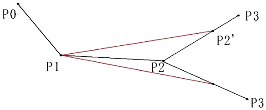
After filtering the path points by the line-of-sight algorithm, a simpler path that removes redundant turns can be obtained and is represented by the path point sequence {P₀, P₁, P₂, …, P_n}. However, there may be turns formed by acute angles in the path obtained using this path to smooth results in excessive path offset. Thus, this article proposes the rotate line algorithm to make angles between path segments as large as possible by adjusting the position of path points between the start and goal. To reduce the collision in this process of moving path points, a middle path point is selected to be moved on the original path segment so that only one path segment where the middle point is located will rotate, and only one edge collision detection is needed. For example, in Figure 3, moving point P₂ on the original path segment (P₂P₃) only rotates one of the path segments where P₂ is located (P₁P₂).

Figure 3.

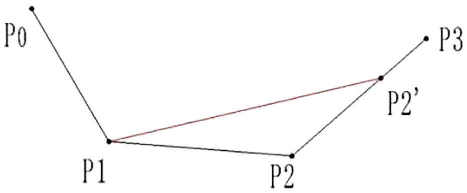
Influence of the moving path middle point on the front angle.

Next, a direction is chosen, and each path point is adjusted so that the angle at each middle point is determined after the next node (or previous node) has been adjusted, that is, the angle of a path point is determined after a double adjustment. For convenience, the angles obtained after the first and second adjustments are referred to as the front and back angles. To ensure that the smoothed path does not deviate too much from the original path, the back angles at all points must be kept greater than the minimum angle: a_min (herein, we set a_min = 90°).

From the start, the position of the path points is adjusted. To meet the abovementioned angle requirement, the influence of adjustment path points on the front and back angles is discussed.

Influence of path point adjustment on the front angle

As shown in Figure 3, considering point P₂′ on the P₂P₃ line segment, the closer P₂′ is to P₃, the greater the angle P₁P₂′P₃ (thus, angle P₁P₂′P₃ = angle P₁P₂P₃ + angle P₂P₁P₂′), and all these angles exceed the angle between P₁P₂ and P₂P₃. Therefore, adjusting the position of point P_i to close to the next path point P_i+₁ can increase the front angle at P_i.

Influence of path point adjustment on back angle

Consider the influence of a path point moving on the back angle. If the vector direction of P₂P₃ is opposite to that of P₁P₀, the back angle P₀P₁P₂′ at P₁ will increase when P₂ moves on line P₂P₃ (as shown by the lower P₃ in Figure 4). However, if the vector direction of P₂P₃ is the same as the direction of P₁P₀, the back angle at P₁ will be reduced, and this reduction will be more obvious as it is closer to point P₃ (higher P₃ in Figure 4).

Figure 4.

Influence of the moving path middle point on the back angle.

Consider the two situations of the back angle change. In the first case, the back angle change at P₁ is consistent with the front angle change at P₂ with the movement of P₂. In the second case, changes in the two angles are opposite. Therefore, considering that the front angle may be reduced as the back angle when the next path point is adjusted, the direction where the front angle becomes larger is selected as the moving direction of P₂ to leave a margin for subsequent adjustments. Simultaneously, considering the back angle requirement, the restriction on the back angle is added when selecting P₂′.

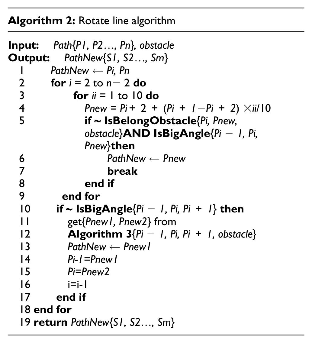
If the minimum angle requirement does not meet the goals after selecting the point that makes the maximum back angle P₂′, the parallel line algorithm described in the next section is proposed to process the back angle to meet the minimum angle requirement. The specific rotate line algorithm process is described in Algorithm 2 (Note that this statement only describes the adjustment method of path midpoints). For the starting point of the path, only the collision detection process is needed. For the path endpoint, an additional angle detection process is needed.

Algorithm 2: Rotate line algorithm
Input: Path{P1, P2…, Pn}, obstacle Output: PathNew{S1, S2…, Sm} 1 PathNew ← Pi, Pn 2 fori = 2 to n− 2 do 3 forii = 1 to 10 do 4 Pnew = Pi+ 2 + (Pi + 1−Pi + 2) ×ii/10 5 if ~ IsBelongObstacle{Pi, Pnew, obstacle}AND IsBigAngle{Pi − 1, Pi, Pnew} then 6 PathNew ← Pnew 7 break 8 end if 9 end for 10 if ~ IsBigAngle{Pi − 1, Pi, Pi + 1} then 11 get{Pnew1, Pnew2} from 12 Algorithm 3{Pi − 1, Pi, Pi + 1, obstacle} 13 PathNew ← Pnew1 14 Pi-1=Pnew1 15 Pi=Pnew2 16 i=i-1 17 end if 18 end for 19 returnPathNew{S1, S2…, Sm}

Algorithm 2: Rotate line algorithm

Input: Path{P1, P2…, Pn}, obstacle
Output: PathNew{S1, S2…, Sm}
1 PathNew ← Pi, Pn
2 fori = 2 to n− 2 do
3 forii = 1 to 10 do
4 Pnew = Pi+ 2 + (Pi + 1−Pi + 2) ×ii/10
5 if ~ IsBelongObstacle{Pi, Pnew, obstacle}AND IsBigAngle{Pi − 1, Pi, Pnew} then
6 PathNew ← Pnew
7 break
8 end if
9 end for
10 if ~ IsBigAngle{Pi − 1, Pi, Pi + 1} then
11 get{Pnew1, Pnew2} from
12 Algorithm 3{Pi − 1, Pi, Pi + 1, obstacle}
13 PathNew ← Pnew1
14 Pi-1=Pnew1
15 Pi=Pnew2
16 i=i-1
17 end if
18 end for
19 returnPathNew{S1, S2…, Sm}

Parallel line algorithm

Figure 5 shows that for the points on line segment P₂P₃, the angle between P₂ and P₁, P₀ (i.e., the back angle of P₁), is the largest, but the angle is still less than the minimum angle required (90°). At this time, the parallel line algorithm is applied.

Figure 5.

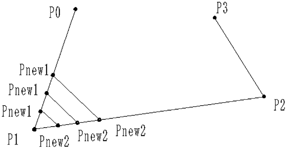
Working principle of the parallel line algorithm.

The main principle of the parallel line algorithm is presented as follows. When the rotate line algorithm moves the path point P_i to its original position, the back angle of P_i₋₁ still does not meet the minimum angle requirement. Find points P_new₁ and P_new₂ on the line segment P_i₋₁P_i₋₂ and the line segment P_i₋₁P_i, respectively. The line segments P_i₋₁P_new₁ and P_i₋₁P_new₂ are equal. In this way, it can be known from the isosceles triangle that the interior angle P_new₁P_new₂P_i = the interior angle P_new₂P_new₁P_i₋₁ > 0°. Thus, it can be ensured that the back angle at P_new₁ (P_new₂P_new₁P_i₋₁) meets the minimum angle requirement. The specific operation steps of the parallel line algorithm are described in Algorithm 3.

Algorithm 3: Parallel line algorithm
Input : Path{P1, P2, P3}, obstacle Output: PathNew{Pnew1, Pnew2} 1 ii = 10 2 MoveStep = Min{length(P1−P2)/2, length(P3−P2)/2}/10 3 whileii < 10 do 4 Pnew1 = P2+ Orientation(from P2 to P1) ×MoveStep×ii 5 Pnew2 = P2+ Orientation(from P2 to P3) ×MoveStep×ii 6 if ~ IsBelongObstacle{Pnew1, Pnew2, obstacle} then 7 break 8 end if 9 ii = ii-1 10 end while 11 returnPathNew{Pnew1, Pnew2}

Algorithm 3: Parallel line algorithm

Input : Path{P1, P2, P3}, obstacle
Output: PathNew{Pnew1, Pnew2}
1 ii = 10
2 MoveStep = Min{length(P1−P2)/2, length(P3−P2)/2}/10
3 whileii < 10 do
4 Pnew1 = P2+ Orientation(from P2 to P1) ×MoveStep×ii
5 Pnew2 = P2+ Orientation(from P2 to P3) ×MoveStep×ii
6 if ~ IsBelongObstacle{Pnew1, Pnew2, obstacle} then
7 break
8 end if
9 ii = ii-1
10 end while
11 returnPathNew{Pnew1, Pnew2}

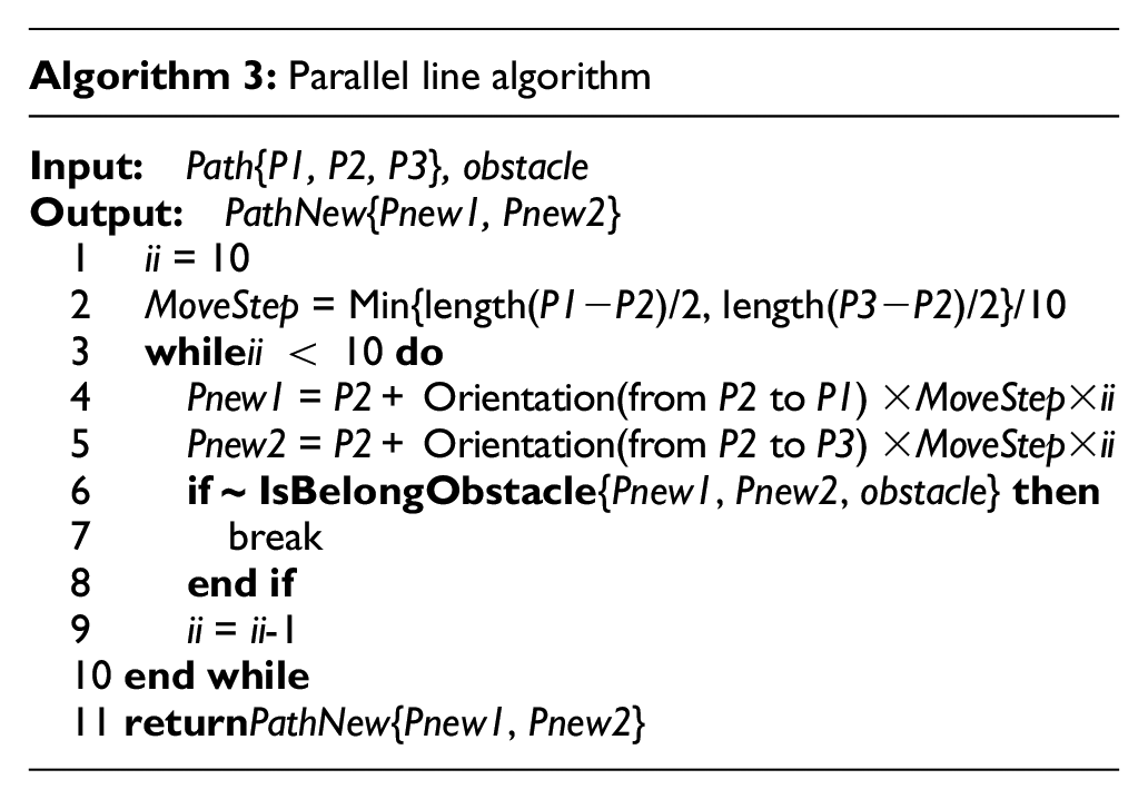
Figure 6 shows the path results after using the path point adjustment algorithm. After operations, the path is smoother, the turns are fewer, and the minimum angle requirement is satisfied.

Figure 6.

Result of the path point adjustment algorithm.

B-spline path smoother acting at turns of path

After processing the path, as described in the first section, the path becomes shorter in length and enables the robot to turn easier. However, the formed path only satisfies C⁰ continuity at the turns, and the robot suddenly changes speed when turning, which is harmful in controlling the robot. Therefore, the processed path needs to be further smoothed. This section proposes a B-spline curve path-smoothing method that acts on the turns of a path. A path is smoothed by inserting the B-spline curve at turns, and the control points of the B-spline curves are adjusted to make the overall smoothed path attain the robotic sport requirements., that is, path continuity, path safety, and path maximum curvature requirements.

B-spline control point selection method for path continuity

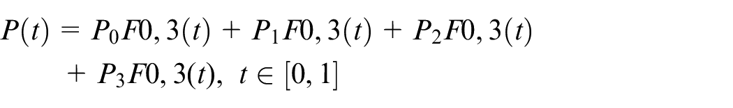
The p-order B-spline curve is C^p-k continuous at the node with a repeat degree of k. To ensure C² continuity at the position of a simple node vector (in which k = 1), at least the cubic B-spline curve must be selected. A considerably high order will result in more calculations and greater deviation from an original path. Herein, the cubic B-spline curve is selected to smooth the path. In addition, the clamped-B-spline curve was used to make the B-spline curve pass through the first and last control points. Therefore, given n + 1 control points P₀, P₁, …, P_n and a node vector U = {u₀, u₁, …, u_m}, the cubic clamped-b-spline curve used in this paper can be expressed as⁴¹:

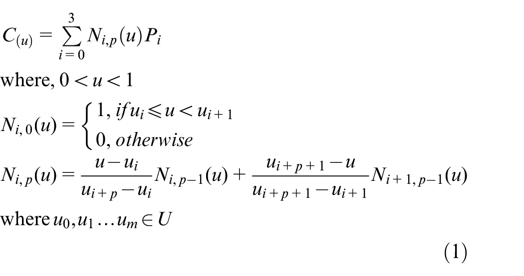
\begin{array}{l} \begin{matrix} C_{(u)} = \sum_{i = 0}^{3} N_{i, p} (u) P_{i} \end{matrix} \\ where ， 0 < u < 1 \\ N_{i, 0} (u) = {\begin{matrix} 1, i f u_{i} \leq u < u_{i + 1} \\ 0, o t h e r w i s e \end{matrix} \\ N_{i, p} (u) = \frac{u - u_{i}}{u_{i + p} - u_{i}} N_{i, p - 1} (u) + \frac{u_{i + p + 1} - u}{u_{i + p + 1} - u_{i + 1}} N_{i + 1, p - 1} (u) \\ where u_{0}, u_{1} \dots u_{m} \in U \end{array}

(1)

We set nine control points (we discuss how to determine and adjust these positions later). Therefore, we can determine that the set U is

U = {0, 0, 0, 0, 1 / 6, 1 / 3, 1 / 2, 2 / 3, 5 / 6, 1, 1, 1, 1}

In some cases (we discuss later), we set eleven control points, and the set U is

U = {0, 0, 0, 0, 1 / 8, 1 / 4, 3 / 8, 1 / 2, 5 / 8, 3 / 4, 7 / 8, 1, 1, 1, 1} .

To smoothly insert the B-spline curve into the proper position of the original path (ensuring continuities C⁰, C¹, and C² at the insertion position is necessary), from the B-spline curve expression, the first derivative function of the B-spline curve can be obtained as:

\frac{d}{du} C_{(u)} = \sum_{i = 0}^{n - 1} N_{i + 1, p - 1} (u) Q_{i}

(2)

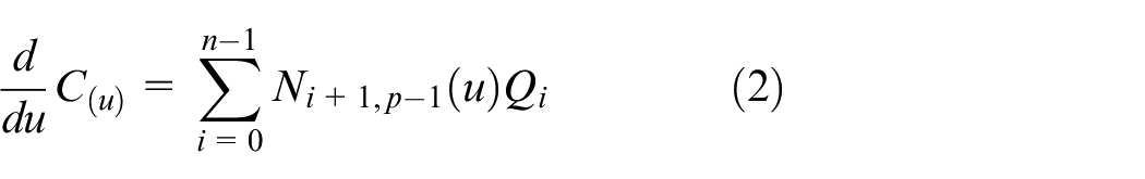
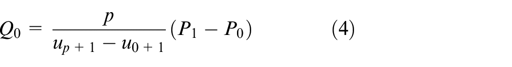
where the expression of Q_i is:

Q_{i} = \frac{p}{u_{i + p + 1} - u_{i + 1}} (P_{i + 1} - P_{i})

(3)

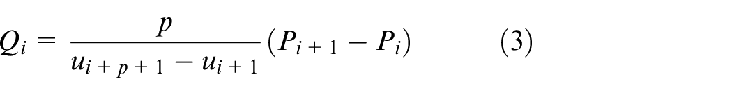
Therefore, the derivative of a clamped-B-spline curve of order p is another clamped-B-spline curve of order p − 1, which is defined by n new control points Q₀, Q₁, …, Q_n₋₁ and a new node vector U′ = {u₁, …, u_m₋₁}, which can be obtained by removing the first and last nodes from the original node vector. The clamped-B-spline curve passing through the first and last control points shows that the first derivative at the first (last) point of the path segment is equal to Q₀ (Q_n₋₁).

Q_{0} = \frac{p}{u_{p + 1} - u_{0 + 1}} (P_{1} - P_{0})

(4)

Q_{n - 1} = \frac{p}{u_{n + p} - u_{n}} (P_{n} - P_{n - 1})

(5)

As seen from the above equations, the derivative of P₀ (P_n₋₁) is in the same direction as the line P₀P₁ (P_n P_n₋₁). We ensure that the direction of P₀P₁ (P_n P_n₋₁) is the same as that of the inserted path to guarantee the C¹ continuity of the inserted position.

The original path is linear, so the second derivative at inserted points is zero. Based on the strong convexity of the B-spline curve. If u is in the node interval [u_i, u_i+₁], then C(u) is in the convex hull of P_i−p, P_i−p₊₁, …, P_i. Thus, for the cubic B-spline curve, if four control points are collinear, the B-spline curve with the second derivative of zero can be constructed, and this curve can be smoothly inserted into the line.

Hence, the four initial {P₁, P₂, P₃, P₄} and last {P₆, P₇, P₈, P₉} points of the B-spline are constrained to be collinear with an original path. Then, the B-spline curve can be smoothly inserted into the original path.

B-spline control point adjustment method for path security

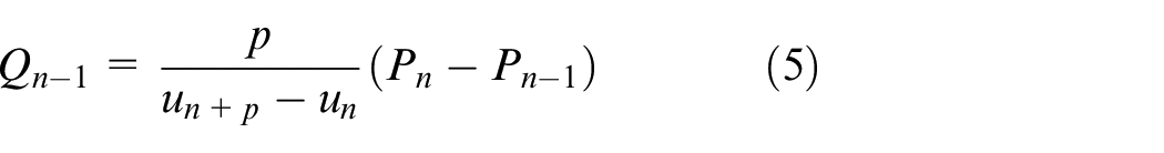
From the above section, to meet the requirement of path continuity, the initial eight control points P₁–P₄, P₆–P₉ are set at each turn in the path distributed on two sides of the turns and make them collinear with the line segments where they are located, and set the control point P₆ at the turns. Only P₄, P₅, and P₆ have a great influence on the shape of the curve due to the segmental nature of the B-spline curve. The closer P₄ and P₆ are to control point P₅, the shorter the length and the smaller the curvature of the generated path. P₃ and P₇ should be set closer to P₄ and P₆ to enhance the restriction of the convex hull on the curve. P₁ and P₉ should comprehensively consider the influence of the length of the line segment and the movement space reserved for P₄ and P₆. The design of the control point position used in this paper is:

{\begin{matrix} P_{1} = P_{t} + v_{t \to t - 1} \times len \times 1 / 2 \\ P_{2} = P_{t} + v_{t \to t - 1} \times len \times 1 / 2 \times 0.99 \\ P_{3} = P_{t} + v_{t \to t - 1} \times len \times 1 / 2 \times 0.51 \\ P_{4} = P_{t} + v_{t \to t - 1} \times len \times 1 / 2 \times 0.5 \\ P_{5} = P_{t} \\ P_{6} = P_{t} + v_{t \to t + 1} \times len \times 1 / 2 \times 0.5 \\ P_{7} = P_{t} + v_{t \to t + 1} \times len \times 1 / 2 \times 0.51 \\ P_{8} = P_{t} + v_{t \to t + 1} \times len \times 1 / 2 \times 0.99 \\ P_{9} = P_{t} + v_{t \to t + 1} \times len \times 1 / 2 \end{matrix}

(6)

where P_t is the position at the turn, $v_{t \to t - 1}$ , $v_{t \to t + 1}$ are the vectors along two sides of the turn, len is the shorter length of two sides at the turn.

To control the B-spline curve to avoid collisions, two points of the control points sequence distributed on each side of a turn are moved until the points on the line segment between these two points do not collide with obstacles. From the convex hull property of the B-spline curve, if the lines connected by the control points do not collide with obstacles, the B-spline curve generated by those points has a high probability of not colliding. Additionally, the experiments found that the farther the collision detection point is from the turns, the shorter the length and the smaller the curvature of the generated path. Therefore, the collision detection points were placed at positions farther from turns, and then the iterative movement was performed in the direction of the turns.

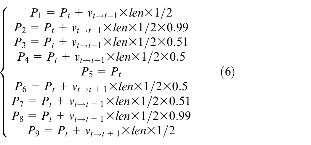
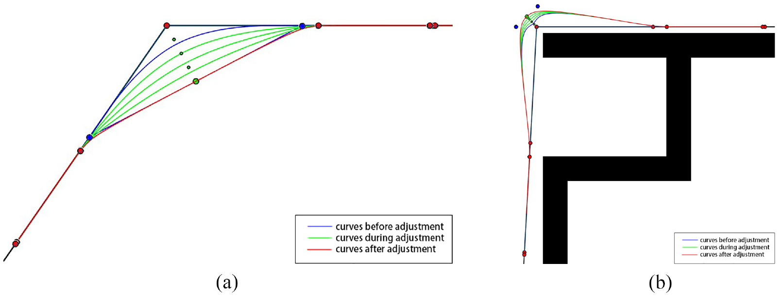
The specific method of moving the control points is described as follows. First, collision detection is performed on the two middle points closest to the position of turns, and if a collision occurs, the detection points set on both sides are moved in the direction of the turns until no collision occurs. When the distance moved by the detection points is too large to make the points exceed the position of turns, the order of the two detection points is exchanged, and new control points are inserted at the starting position of the moving points. Figure 7 shows that after moving two detection points, the newly generated path no longer collides with obstacles. Figure 7(a) is the general situation, and Figure 7(b) is the situation when the collision detection points exceed the turns. The red points and the curve are the positions of the control points and corresponding curve shape before adjustment, the green points and curves are the positions of the collision detection points and corresponding curve shapes during the adjustment process, and the blue points and curve are the positions of the collision detection points after the adjustment process and corresponding curve shape.

Figure 7.

Process of moving collision detection points: (a) the situation of detection points that do not exceed the turn and (b) the situation of detection points exceeding the turn.

B-spline control point adjustment method for the maximum curvature of a path

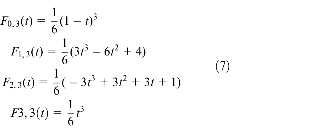
From the nature of the B-spline curve, it can be seen that the shape of a third-degree B-spline curve is determined by a control point sequence composed of four control points. In the previous steps, we set nine control points to generate a B-spline curve. According to the control point sequence that determines the shape of a control curve, the generated B-spline curve can be divided into six segments. Among them, due to the symmetry, these segments can be simplified into two cases, that is, Case 1: four control points are on a line segment, Case 2: three control points are on a line segment, and the remaining control point is outside the line segment. The curve segment generated in Case 1 is a line segment with a constant curvature value of 0. We mainly discuss the curvature of the point on a curve segment under Case 2. The control point sequence of Case 2 can be described in the Cartesian coordinate system as P₀(0, 0), P₁(a, 0), P₂(b, 0), P₃(b+(b − a)cos(α), (b − a)sin(α)), which can be seen in Figure 8. We plug the definition of a uniform B-spline curve (given by equation (7)) by the coordinates of control points P₀, P₁, P₂, and P₃ to yield the expression of the B-spline curve segment in Cartesian coordinates.

\begin{matrix} P (t) = P_{0} F 0, 3 (t) + P_{1} F 0, 3 (t) + P_{2} F 0, 3 (t) + P_{3} F 0, 3 (t), t \in [0, 1] \end{matrix}

where

\begin{matrix} F_{0, 3} (t) = \frac{1}{6} (1 - t)^{3} \\ F_{1, 3} (t) = \frac{1}{6} (3 t^{3} - 6 t^{2} + 4) \\ F_{2, 3} (t) = \frac{1}{6} (- 3 t^{3} + 3 t^{2} + 3 t + 1) \\ F 3, 3 (t) = \frac{1}{6} t^{3} \end{matrix}

(7)

\begin{matrix} x = \frac{1}{6} (3 t^{3} - 6 t^{2} + 4) a + \frac{1}{6} ((- 3) t^{3} + 3 t^{2} + 3 t + 1) b \\ + \frac{1}{6} t^{3} (b + (b - a) \cos (α)) \\ y = \frac{1}{6} t^{3} (b - a) \sin (α) \end{matrix}

(8)

Figure 8.

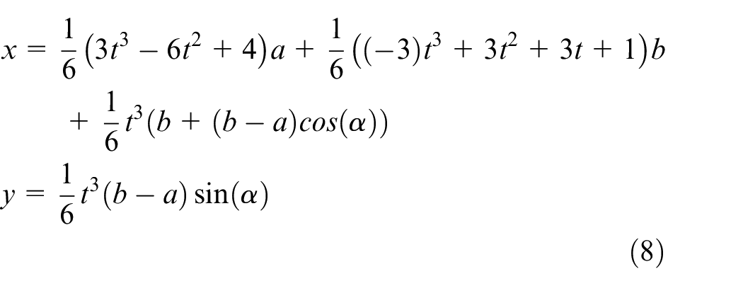
The control point sequence of Case 2.

The curvature value at the position of parameter t in the curve segment is calculated by the curvature formula given by equation (9):

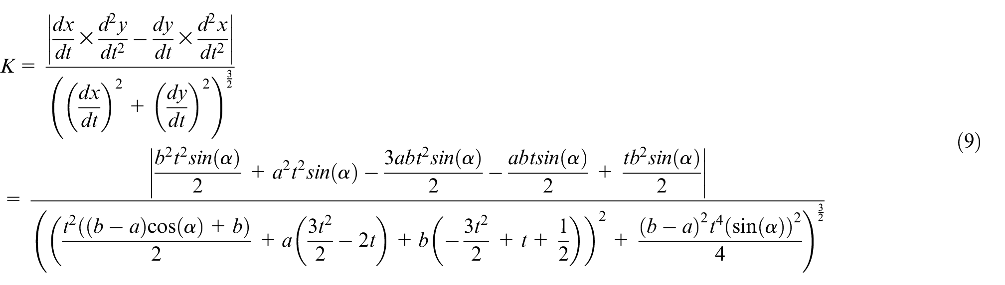
\begin{matrix} K = \frac{| \frac{dx}{dt} \times \frac{d^{2} y}{d t^{2}} - \frac{dy}{dt} \times \frac{d^{2} x}{d t^{2}} |}{{({(\frac{dx}{dt})}^{2} + {(\frac{dy}{dt})}^{2})}^{\frac{3}{2}}} \\ = \frac{| \frac{b^{2} t^{2} \sin (α)}{2} + a^{2} t^{2} \sin (α) - \frac{3 ab t^{2} \sin (α)}{2} - \frac{abtsin (α)}{2} + \frac{t b^{2} \sin (α)}{2} |}{{({(\frac{t^{2} ((b - a) \cos (α) + b)}{2} + a (\frac{3 t^{2}}{2} - 2 t) + b (- \frac{3 t^{2}}{2} + t + \frac{1}{2}))}^{2} + \frac{{(b - a)}^{2} t^{4} {(\sin (α))}^{2}}{4})}^{\frac{3}{2}}} \end{matrix}

(9)

To simplify processing, the above formula is squared, and the square of the curvature value at parameter t is plotted, as shown in Figure 9. It should be noted that the parameters in Figure 9 are set as a = 1, b = 2, and the angle of rotation α = 1. In fact, the same conclusion can be obtained for any situation where b > a. It can be seen that the larger the value of parameter t is, the larger the curvature value. Next, we take t as 1 and use the above formula to derive α to consider the influence of the rotation angle α on the maximum curvature value. We plot the derivative of the square of the curvature value at the rotation angle α, as shown in Figure 10. It can be seen that in the interval [0, π], the maximum curvature value increases with an increasing rotation angle, that is, the smaller the angle between the line segments is, the greater the maximum curvature value.

Figure 9.

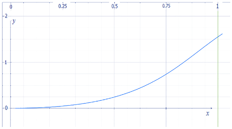
The square of the curvature value at parameter t.

Figure 10.

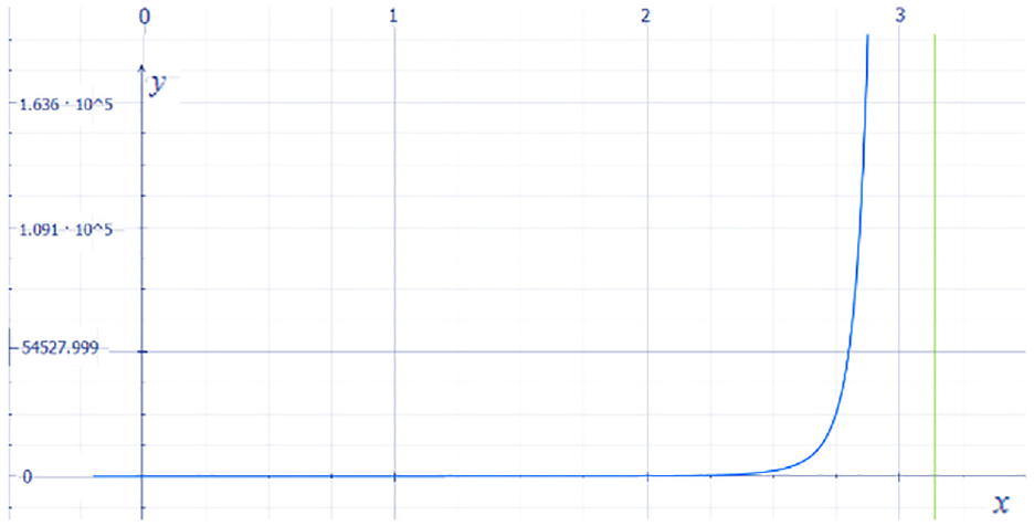
The derivative of the square of the curvature value at rotation angle α.

After the path point adjustment algorithm proposed in the first section is implemented, the angles between path segments increased and exceeded the set value. The curvature of the B-spline curves with control points on this path is smaller than that on an original path. On this basis, we conduct experiments on the effect of moving the control point at the turns of the control point sequence under different parameter values, as shown in Figure 11. We simplify the control points and only intercept the control point sequence corresponding to the middle section of the curve where the maximum curvature value appears, that is, P₀(0, 8), P₁(0, 6), P₂(0, 0), P₃ (6, 0), and P₄ (8, 0). When the initial control point sequence set in the above steps is adopted, we gradually move point P₂, as shown in Figure 11(a), and draw the curvature change of the curve, as shown in Figure 11(b). Before moving point P₂, the maximum curvature value in the curve segment appears at position t = 0.5. Moving the control point along the direction of the angle bisector can reduce the curvature value at this position (t = 0.5), but it will increase the curvature value at other positions, and the maximum curvature value of the overall curve segment decreases and shortens the length of the curve. In the next step, we further smooth the curve and reduce the maximum curvature by adopting the above method, which moves the control points at turns of a path.

Figure 11.

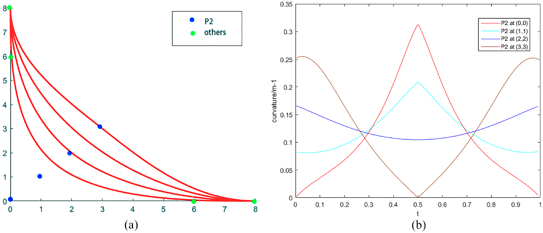
The curvature and shape of the curve in the process of moving point P₂: (a) the shape of the curve and (b) the curvature of the curve.

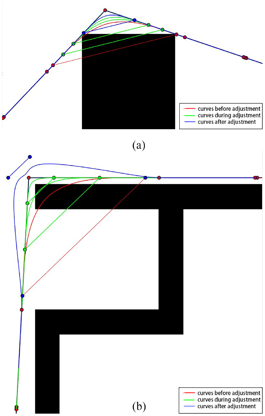
After obtaining the position of collision detection points, which meets the requirement of a collision-free path, the control points set at turns of a path are gradually moved toward the line segment formed by connecting the collision detection points. Simultaneously, collision detection on the B-spline curve is performed. If no collision occurs, the control point will be continuously moved until a collision occurs or it reaches the line segment containing the collision detection point. Figure 12 shows that by moving the control point at the turning point, a smoother unobstructed path is obtained; the path length decreases, and the curve becomes smoother. Figure 12(a) depicts the general situation, and Figure 12(b) depicts the situation when the collision detection points exceed the turns. The red points are the initial control points, and the blue points are the control points that change after the method is adjusted in the previous section. The green points are the change in the control point position during and after the moving process. The blue curve is the shape of the curve adjusted by the method in the previous section, the green curves are the change in the curve shape during the moving process, and the red curve is the final curve shape after the moving process.

Figure 12.

Process of moving the B-spline control point set at a turn: (a) the situation of detection points does not exceed the turn and (b) the situation of detection points exceeding the turn.

Experiments

A simulation experiment is conducted on a computer with an i7-10875h CPU @ 2.30 GHz using MATLAB 2020b. The map is defined as a grid map composed of square cells. Each square cell has two states of 0 and 1 to indicate whether a robot can pass. To test the performance of the proposed path point adjustment algorithm and the overall algorithm (PAATS) in different environments and their adaptability to different path planning algorithms, three different maps are set up where PAATS and the path point adjustment algorithm are simulated independently combined with the RRT⁴² and A*⁴³ algorithms. Next, the PAATS algorithm are compared with other mainstream smoothing algorithms on the first map.

Figure 13 shows that three maps are set up to simulate indoor, clutter and large indoor, and random obstacle environments. Among them, black indicates an obstacle that is not allowed to pass, whereas white indicates one that is allowed to pass. Next, the start and goal of a 50 × 50-pixel map are set as (46, 4) and (9, 47), respectively. Additionally, the start and goal of a 150 × 150-pixel map are set as (8, 7) and (132, 135), respectively.

Figure 13.

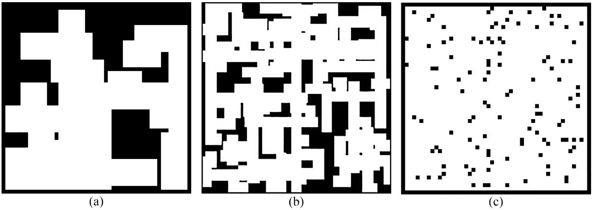
Simulation map construction: (a) 50 × 50-pixel, (b) 50 × 50-pixel, and (c) 50 × 50-pixel.

Path point adjustment algorithm experiment

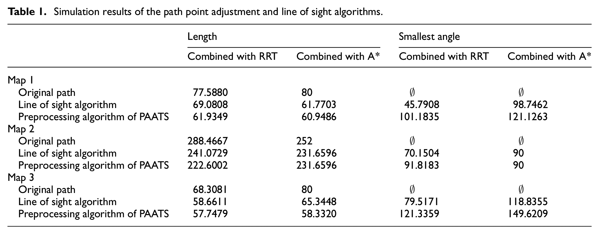
On three different maps, the initial point and the target point are set according to the information mentioned above, and the corresponding paths are calculated by the A* algorithm and the RRT algorithm, respectively. The RRT algorithm runs repeatedly, and 100 corresponding paths are calculated. Then, the solved path is processed by the line-of-sight algorithm and the path point preprocessing algorithm proposed in this paper, and the effectiveness of this method is verified by comparison. The experimental results obtained are shown in Table 1, among which the length in the record of the RRT algorithm is the average result of multiple experiments, and the angle is the minimum value in multiple experiments. Therefore, the proposed algorithm can increase the angles of a path above the set minimum angle and decrease the path length.

Table 1.

Simulation results of the path point adjustment and line of sight algorithms.

	Length		Smallest angle
	Combined with RRT	Combined with A*	Combined with RRT	Combined with A*
Map 1
Original path	77.5880	80	∅	∅
Line of sight algorithm	69.0808	61.7703	45.7908	98.7462
Preprocessing algorithm of PAATS	61.9349	60.9486	101.1835	121.1263
Map 2
Original path	288.4667	252	∅	∅
Line of sight algorithm	241.0729	231.6596	70.1504	90
Preprocessing algorithm of PAATS	222.6002	231.6596	91.8183	90
Map 3
Original path	68.3081	80	∅	∅
Line of sight algorithm	58.6611	65.3448	79.5171	118.8355
Preprocessing algorithm of PAATS	57.7479	58.3320	121.3359	149.6209

Overall algorithm (PAATS) experiment

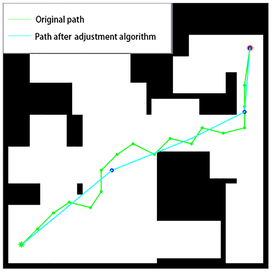
Figure 14 shows the experimental results of the overall algorithm in Map 1. The original path obtained using the path planning algorithm is displayed in green, the path after implementing the path point adjustment algorithm is displayed in blue, and the turn segment in the path processed using the turn-smoothing method is displayed in red. It can be seen intuitively that the path processed using the PAATS algorithm avoids obstacles and remains continuous and smooth, and the smoothed path has a high fit with an original path. In Figure 15, each curve segment in the path using the turn-smoothing method is intercepted at 200 points in length, and the curvature value of those points is calculated. In addition, the path processed using the PAATS algorithm can meet the C² continuity requirement.

Figure 14.

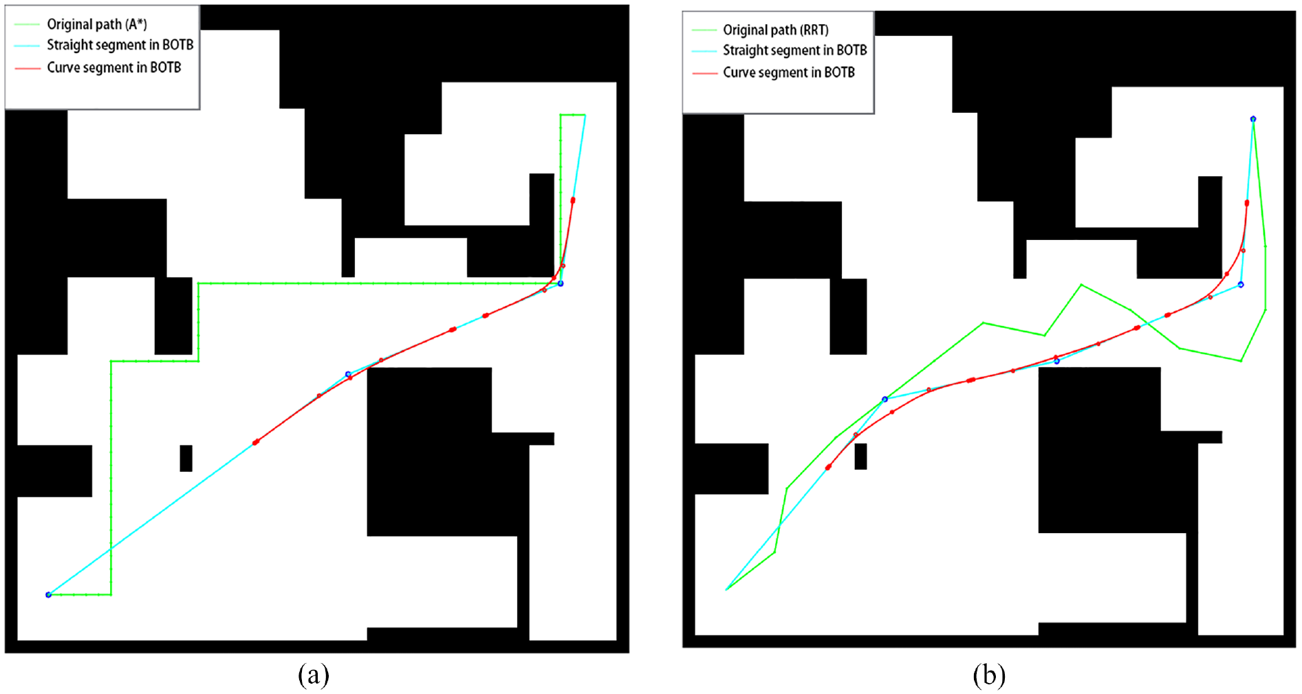
PAATS result in Map 1: (a) the result connected with the RRT algorithm and (b) the result connected with the A* algorithm.

Figure 15.

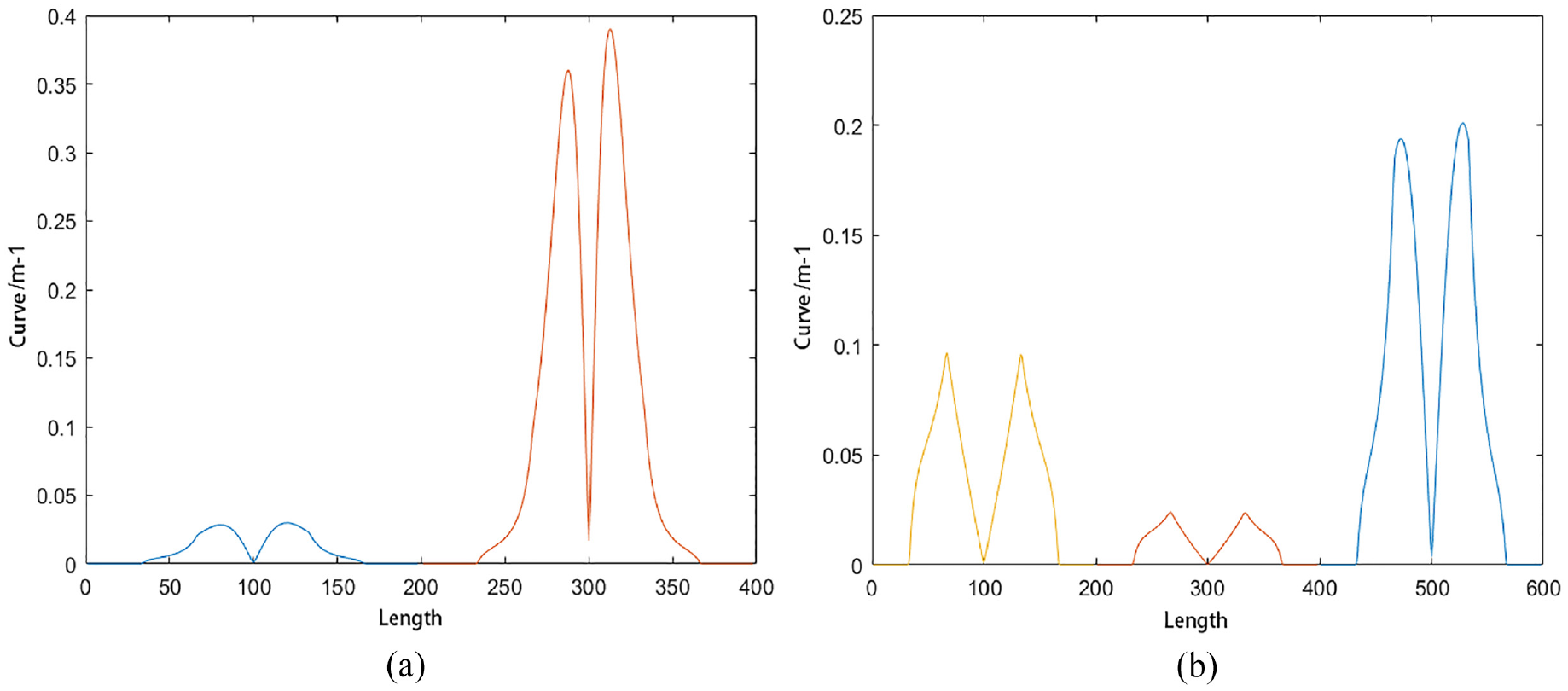
Curvature of curve segments in the path obtained by PAATS in Map 1: (a) the result connected with the RRT algorithm and (b) the result connected with the A* algorithm.

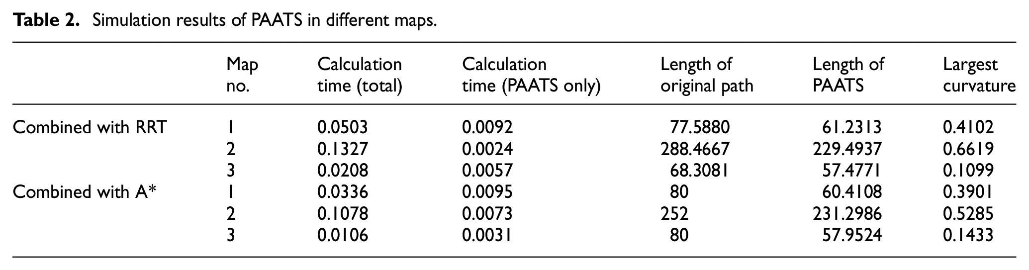
On three different maps, the initial point and the target point are set according to the information mentioned above, and the corresponding paths are calculated by the A* algorithm and the RRT algorithm, respectively. The RRT algorithm runs repeatedly, and 100 corresponding paths are calculated. Afterwards, the smoothing algorithm proposed in this paper is used to process the solved path to verify the validity of this method. The experimental results obtained are shown in Table 2, and the records of the RRT algorithm are the average results of multiple experiments. The PAATS algorithm can be combined with the A* or RRT algorithm to obtain a path with a short length. Additionally, with the PAATS algorithm, the maximum curvature satisfies the requirements of robot motion in different scenes and map sizes, and the smoothing algorithm takes much less time than the path planning process to meet the real-time performance of the motion of the robot.

Table 2.

Simulation results of PAATS in different maps.

	Map no.	Calculation time (total)	Calculation time (PAATS only)	Length of original path	Length of PAATS	Largest curvature
Combined with RRT	1	0.0503	0.0092	77.5880	61.2313	0.4102
	2	0.1327	0.0024	288.4667	229.4937	0.6619
	3	0.0208	0.0057	68.3081	57.4771	0.1099
Combined with A*	1	0.0336	0.0095	80	60.4108	0.3901
	2	0.1078	0.0073	252	231.2986	0.5285
	3	0.0106	0.0031	80	57.9524	0.1433

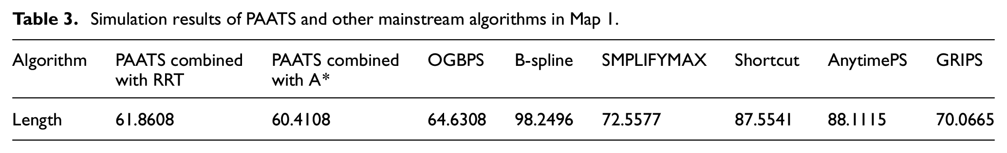
In the 50 × 50 map environment, this algorithm is compared with other path-smoothing algorithms (OGBPS,³⁰ GRIPS,²⁸ B-spline,⁴⁴ Shortcut,⁴⁵ SimplifyMax, Anytime PS⁴⁶). Figure 16 compares the results. Additionally, Table 3 shows that the path calculated using the PAATS algorithm is better in length, and the path is more reasonable and conducive to driving a robot.

Figure 16.

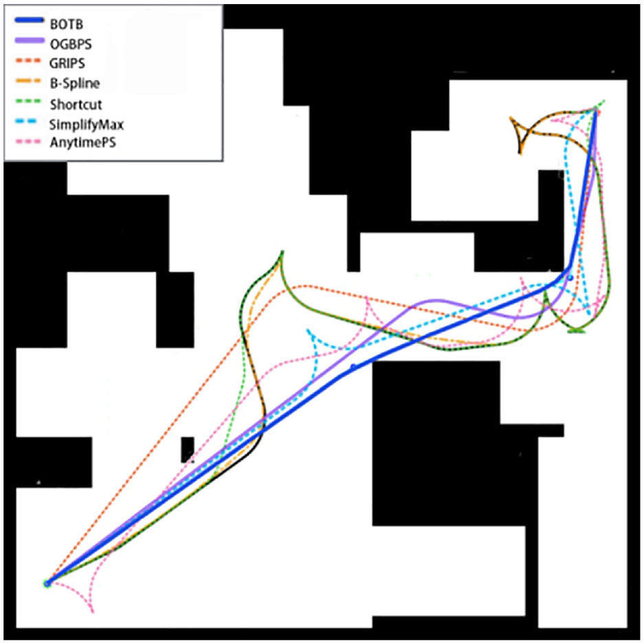
Comparison between PAATS and other mainstream algorithms in Map 1.

Table 3.

Simulation results of PAATS and other mainstream algorithms in Map 1.

Algorithm	PAATS combined with RRT	PAATS combined with A*	OGBPS	B-spline	SMPLIFYMAX	Shortcut	AnytimePS	GRIPS
Length	61.8608	60.4108	64.6308	98.2496	72.5577	87.5541	88.1115	70.0665

Conclusion

This paper proposes a path smoothing algorithm that consists of two parts, that is, the path point preprocessing algorithm and the B-spline path smoother algorithm. Among them, the path point preprocessing algorithm adjusts the position of the path point to remove unnecessary turns in the path and increases the angle between the linear paths. The B-spline path smoother algorithm only smooths the turns of the original path to improve efficiency of the algorithm and to reduce the deviation from the original path. Moreover it adjusts the position of the control points of the B-spline curve to further improve the performance of the path. Overall, this algorithm can smooth the piecewise linear path and obtain an unobstructed path that satisfies the c2 continuity and maximum curvature constraints. In the simulation experiment, the algorithm proposed in this paper is compared with other path smoothing algorithms, and it is proven that the path proposed by this algorithm is shorter in length and easier for the robot to travel.

Future work would entail evaluating different paths in advance and choosing the best path for smoothing. Especially in a narrow environment, a piecewise linear path can be found, but no path may satisfy the smooth condition.

Footnotes

Author contributions

All authors contributed to the study conception and design. NC, GY, SZ contributed to the conception of the study. NC performed the experiment. NC, GY contributed significantly to analysis and manuscript preparation. NC performed the data analyses and wrote the manuscript. NC, GY, SZ, LQ helped perform the analysis with constructive discussions.

Declaration of conflicting interests

The author(s) declared no potential conflicts of interest with respect to the research, authorship, and/or publication of this article.

Funding

The author(s) disclosed receipt of the following financial support for the research, authorship, and/or publication of this article: Project supported by the National Key Research and Development Program of China, grant number 2019YFC1511502, the National Natural Science Foundation of China, grant number 51875515, the Science and Technology Program of Zhejiang Province, grant number 2021C01149, and the Science and Technology Program of Beijing, grant number Z191100001419014.

Consent to participate

All mentioned authors voluntarily agreed to participate in this research topic.

Consent to publish

The authors and relevant institutions approve publishing this research.

ORCID iD

Guodong Yi

Data,materials and/or code availability

The data used to support the findings of this study are available from the corresponding author upon request.

References

Wallace

Stentz

Thorpe

, et al. First results in robot road following. Comput Eng Proc Int Comput Eng Conf 1985; 1: 381–387.

Antonelli

Chiaverini

Fusco

A fuzzy-logic-based approach for mobile robot path tracking. IEEE Trans Fuzzy Syst 2007; 15(2): 211–221.

Marzbani

Quốc

, et al. Autodriver autonomous vehicles control strategy. Procedia Comput Sci 2018; 126: 870–877.

Zeng

Xiong

, et al. A steerable curvature approach for efficient executable path planning for on-road autonomous vehicle. SAE paper 2019-01-0675. 2019.

Yang

. AUV path planning based on improved RRT and Bezier curve optimization. In: 2020 IEEE International Conference on Mechatronics and Automation (ICMA), Beijing, China, 13–16 October 2020, pp.1359–1364. New York, NY: IEEE.

Qiao

Zheng

Wang

. A path planning method for autonomous ships based on SVM. In: Proceedings of the 32nd Chinese control and decision. Conference (CCDC), Hefei, China, 22–24 August 2020, pp. 3068–3072. Bristol: IOP.

Huang

Cao

Zhu

Mixed path planning for multi-robots in structured hospital environment. J Eng 2019; 14: 512–516.

Pivtoraiko

Kelly

Efficient constrained path planning via search in state lattices. In: Proceedings of 8th international symposium on artificial intelligence, robotics and automation in space (iSAIRAS ‘05), Munich, 5–8 September 2005, pp.249–255. Paris: European Space Agency (Special Publication).

Masehian

Sedighizadeh

. A multi-objective PSO-based algorithm for robot path planning. In: 2010 IEEE international conference on industrial technology, Via del Mar, Chile, 14–17 March 2010, pp.465–470. New York, NY: IEEE.

10.

Zhao

Xia

Global path planning based on simultaneous visibility graph construction and A* algorithm. J Nanjing Univ Sci Technol 2017; 41(3): 313–321.

11.

LaValle

Kuffner

JJ.

Randomized kinodynamic planning. Int J Rob Res 2001; 20(5): 378–400.

12.

Kavraki

Kolountzakis

Latombe

JC.

Analysis of probabilistic roadmaps for path planning. IEEE Trans Robot Autom 1998; 14(1): 166–171.

13.

Anipulators and FORM and Robots

. Real-time obstacle avoidance for manipulators and mobile robots. Int J Rob Res 1986; 5: 500–505.

14.

Sun

DWK

, et al. Optimal 3D-trajectory design and resource allocation for solar-powered UAV communication systems. IEEE Trans Commun 2019; 67(6): 4281–4298.

15.

Zeng

Zhang

Trajectory design for completion time minimization in UAV-enabled multicasting. IEEE Trans Wirel Commun 2018; 17(4): 2233–2246.

16.

Dubins

LE.

On curves of minimal length with a constraint on average curvature, and with prescribed initial and terminal positions and tangents. Am J Math 1957; 79(3): 497.

17.

Reeds

Shepp

KA.

Optimal paths for a car that goes both forwards and backwards. Pacific J. Math. 1990; 145(2): 1990. https://github.com/BasGeertsema/rsmotion%0Ahttps://github.com/nathanlct/reeds-shepp-curves

18.

Khatib

Jaouni

Chatila

, et al. Dynamic path modification for car-like nonholonomic mobile robots. In: Proceedings of international conference on robotics and automation, Albuquerque, NM, 25–25 April 1997, pp.2920–2925. New York, NY: IEEE.

19.

Komoriya

Tanie

Trajectory control of a wheel-type mobile robot using B-spline curve. J Robot Soc Japan 1990; 8(2): 133–143.

20.

Eren

Fung

Evans

. Implementation of the spline method for mobile robot path control. In: IMTC/99. Proceedings of the 16th IEEE instrumentation and measurement technology conference (Cat. No.99CH36309), Venice, 24–26 May 1999, vol. 2, pp. 739–744. New York, NY: IEEE.

21.

Fraichard

Ahuactzin

. Smooth path planning for cars. In: Proceedings 2001 ICRA. IEEE international conference on robotics and automation (Cat. No.01CH37164), Seoul, Korea (South), 21–26 May 2001, vol. 4, pp. 3722–3727. New York, NY: IEEE.

22.

Goerzen

Kong

Mettler

A survey of motion planning algorithms from the perspective of autonomous UAV guidance. J Intell Robot Syst 2010; 57(1–4): 65.

23.

Wang

Liu

, et al. A review on carrier aircraft dispatch path planning and control on deck. Chin J Aeronaut 2020; 33(12): 3039–3057.

24.

Fnadi

Gomes Da Silva

, et al. Local obstacle-skirting path planning for a fast bi-steerable rover using Bézier curves. In: 2020 IEEE international conference on robotics and automation (ICRA), Paris, France, 31 May 2020–31 August 2020, pp. 10242–10248. New York, NY: IEEE.

25.

Elmokadem

. Real-time safe navigation strategy for mobile robots in 3D: a deforming path approach. In: 2019 Chinese control conference (CCC), Guangzhou, China, 27–30 July 2019, pp. 3833–3838. New York, NY: IEEE.

26.

Ravankar

Kobayashi

, et al. Path smoothing extension for various robot path planners. In: 2016 16th international conference on control, automation and systems (ICCAS), Gyeongju, Korea (South), 16–19 October 2016, pp. 263–268. New York, NY: IEEE.

27.

Tian

Yang

, et al. Local smooth path planning for turning around in narrow environment. In: 2019 IEEE 28th international symposium on industrial electronics (ISIE), Vancouver, BC, Canada, 12–14 June 2019, pp. 1924–1929. New York, NY: IEEE.

28.

Choi

Curry

Elkaim

. Path planning based on bézier curve for autonomous ground vehicles. In: Advances in electrical and electronics engineering: IAENG special edition of the world congress on engineering and computer science 2008, San Francisco, CA, USA, 22–24 October 2008. pp. 158–166. New York, NY: IEEE.

29.

Caldeira

Vasconcelos

JVR

Sarcinelli-Filho

, et al. UAV path-following strategy for crossing narrow passages. In: 2020 international conference on unmanned aircraft systems (ICUAS), Athens, Greece, 1–4 September 2020, pp. 26–31. New York, NY: IEEE.

30.

Elbanhawi

Simic

Jazar

Randomized bidirectional B-spline parameterization motion planning. IEEE Trans Intell Transp Syst 2016; 17(2): 406–419.

31.

Luo

Sun

. An optimization-based motion planning method for autonomous driving vehicle. In: 2020 3rd international conference on unmanned systems (ICUS), Harbin, China, 27–28 November 2020, pp. 739–744. New York, NY: IEEE.

32.

Heiden

Palmieri

Koenig

, et al. Gradient-informed path smoothing for wheeled mobile robots. In: 2018 IEEE international conference on robotics and automation (ICRA), Brisbane, QLD, Australia, pp. 1710–1717. New York, NY: IEEE.

33.

Wang

Zhou

. OGBPS: orientation and gradient based path smoothing algorithm for various robot path planners. In: 2019 IEEE international conference on robotics and biomimetics (ROBIO), Dali, China, 6–8 December 2019, pp.1453–1458. New York, NY: IEEE.

34.

Wang

Liu

Peng

, et al. A simultaneous planning and control method integrating APF and MPC to solve autonomous navigation for USVs in unknown environments. J Intell Robot Syst Theory Appl 2022; 105(2): 36.

35.

Cimurs

Suh

IH.

Time-optimized 3D path smoothing with kinematic constraints. Int J Control Autom Syst 2020; 18(5): 1277–1287.

36.

Yang

Miao

, et al. A new robot navigation algorithm based on a double-layer ant algorithm and trajectory optimization. IEEE Trans Ind Electron 2019; 66(11): 8557–8566.

37.

Shiller

Dubowsky

Robust computation of path constrained time optimal motions. IEEE Trans Robot 2004; 20(6): 144–149.

38.

Maekawa

Noda

Tamura

, et al. Curvature continuous path generation for autonomous vehicle using B-spline curves. CAD Comput Aided Des 2010; 42(4): 350–359.

39.

Elbanhawi

Simic

Jazar

RN.

Continuous path smoothing for car-like robots using B-spline curves. J Intell Robot Syst Theory Appl 2015; 80: 23–56.

40.

Elbanhawi

Simic

Randomised kinodynamic motion planning for an autonomous vehicle in semi-structured agricultural areas. Biosyst Eng 2014; 126: 30–44.

41.

Malakiyeh

Shojaee

Hamzehei Javaran

Insight into an implicit time integration method based on Bezier curve and third-order Bernstein basis function for structural dynamics. Asian J Civ Eng. 2018; 19(1): 1–11.

42.

LaValle

Kuffner

JJ.

Rapidly-exploring random trees: progress and prospects. In: Algorithmic and computational robotics, Boca Raton, Fl: CRC Press, 2000, pp.293–308.

43.

Hart

Nilsson

Raphael

Formal basis for the heuristic determination eijj. Syst Sci Cybern 1968; 4(2): 100–107.

44.

Yang

Sukkarieh

An analytical continuous-curvature path-smoothing algorithm. IEEE Trans Robot 2010; 26(3): 561–568.

45.

Hsu

Latombe

Sorkin

. Placing a robot manipulator amid obstacles for optimized execution. In: Proceedings of the 1999 IEEE international symposium on assembly and task planning (ISATP’99) (Cat. No.99TH8470), Porto, Portugal, 24–24 July 1999, pp. 280–285. New York, NY: IEEE.

46.

Luna

Sucan

Moll

, et al. Anytime solution optimization for sampling-based motion planning. In: 2013 IEEE international conference on robotics and automation, Karlsruhe, Germany, 6–10 May 2013, pp. 5068–5074. New York, NY: IEEE.

A multiobjective path-smoothing algorithm based on node adjustment and turn-smoothing

Abstract

Keywords

Introduction

Environmental description and problem definition

Environmental description

Problem definition

The whole process

A path point adjustment algorithm for increasing angles between path segments

Line of sight algorithm

Rotate line algorithm

Influence of path point adjustment on the front angle

Influence of path point adjustment on back angle

Parallel line algorithm

B-spline path smoother acting at turns of path

B-spline control point selection method for path continuity

B-spline control point adjustment method for path security

B-spline control point adjustment method for the maximum curvature of a path

Experiments

Path point adjustment algorithm experiment

Overall algorithm (PAATS) experiment

Conclusion

Footnotes

Author contributions

Declaration of conflicting interests

Funding

Consent to participate

Consent to publish

ORCID iD

Data,materials and/or code availability

References