
Abstract
Developing a fully automatic auxiliary flying system with robot maneuvering is feasible. This study develops a control vision system that can read all kind of needle-type meters. The vision device in this study implements a modified YOLO-based object detection model to recognize the airspeed readings from the needle-type dashboard. With this approach, meter information in the cockpit is replaced by a single camera and a powerful edge-computer for future autopilot maneuvering purpose. A modified YOLOv4-tiny model by adding the Spatial Pyramid Pooling (SPP) and the Bidirectional Feature Pyramid Network (BAFPN) to the Neck region of the convolutional neural networks (CNN) structure is implemented. The Taguchi method for acquiring a set of optimum hyperparameters for the CNN is applied. An improved deep learning network with higher Mean Average precision (mAP) compared with conventional YOLOv4-tiny and possessing a higher Frames Per Second (FPS) value than YOLOv4 is deployed successfully. Established a self-control system using a camera to receive airspeed indications from the designed virtual needle-type dashboard. Moreover, the dashboard’s pointer is controlled by applying the proposed control method, which contains PID control in addition to the pointer’s rotation angle recognition. A modified YOLOv4-tiny model with a fabricated system for visual dynamical recognition control is implemented successfully. The feasibility of bettering mean accuracy precision and frame per second in achieving autopilot maneuvering is verified.
Introduction
Nowadays, taking flights or riding on a helicopter is common transportation for the public. However, under adverse weather conditions or long-haul flying trips, piloting aircraft is a challenging task for human pilots. Both factors may lead to fatigue and misjudgment in pilots. From many investigated accidents, developing a fully automatic auxiliary flying system and installing it in the cockpit to relieve the burden of human pilots and prevent tragedies from happening is imperative.
Sensing technology is a major component for an auxiliary flying system to operate. With the advancement of sensing technology, the majority of current sensors are sufficient to help the autopilot system receive all kinds of flight data coming from the aircraft itself or the flying environment. Required sensing instruments are not only expensive but also invasive to the aircraft when installing. This leads to an inspiration to develop another sensing approach that can solve the problem while being suitable when plug-in device can be embedded with the autopilot system.
The idea is to instruct computers to read flight data as humans do. Applying robot vision to this matter can not only fulfill the purpose but also operating at a lower cost. The advantage of using robot vision on an aircraft is that upon receiving the analog-like dashboard meter then it can immediately transform the data into digital form. It allows us to receive flight data in real-time or even simultaneously stream it back to the air-traffic control tower for investigation in case of a flight accident or any flight control purposes. Moreover, in this research, robot vision only requires a single camera, which replaces the need for multiple sensors. It helps to greatly lower the cost of data reading.
As for processing the information received from robot vision, edge-computing is a requirement for the reason that the cockpit is not usually big enough to install a computer with high computing power. In Ahmad et al., 1 using the NVIDIA Jetson Nano developer kit for real-time detection is feasible. Pathak and Singh 2 adopt NVIDIA Jetson Nano as a health monitoring device, which shows that the NVIDIA Jetson nano is stable enough to execute long-hour monitoring tasks. These two papers demonstrate that with the powerful GPUs equipped within, it is practicable to deploy the NVIDIA Jetson Nano as an edge-computer.
In Li et al., 3 the BAFPN improved the detection ability by replacing the Path Aggregation Network (PANet) 4 structure in the original You Only Look Once version 4 (YOLOv4). This has increased both the calculation speed and accuracy, and it showed a great performance in both mAP and FPS by the Microsoft Common Objects in Context (MS COCO) dataset. However, the detection speed of using CNN model fails to meet the demand for real-time detection. Hence, we will design for the modification of the CNN model in order to balance between accuracy and detection speed. Besides, Su et al. 5 stated that they had applied the BAFPN to YOLOv3 and compared with other CNN structures. The result in Su et al. 5 shows that integrating BAFPN to the CNN structure can lead to great improvement in terms of accuracy. In fact, it has proven to be the most accurate model among other CNN structures. Nonetheless, the BAFPN still has its drawbacks. As, it has been mentioned in Su et al. 5 that BAFPN performs poorly when it comes to deal with detection speed. Hence, to ameliorate a modified CNN structure has become one of the main focus of this paper.
The fully automatic auxiliary flying system consists of two major parts, one is the detection toward the aircraft’s condition, the other is the capability of controlling multiple actuators within the cockpit. Thus, another major concentration in this paper is to validate the feasibility of implementing robot vision to a control system apparatus. Taking the detection results as input, followed by numerous calculations, and a control signal output for the apparatus to operate functionally will be achieved. In addition, a needle-type dashboard was included to display measured airspeed in our verification experiment. Needle-type dashboards are often used in industrial manufacturing, military, aerospace, and other fields for data monitoring. However, readings from the needle-type dashboard are harder to acquire than those displayed on a digital meter, since the former only outputs analog data and possesses no data transmitting portal. Therefore, we digitized the analogous airspeed data by using a camera to record the dashboard’s display and via a deep learning network to output the speed recognition.
Basis of YOLO deep learning networks
YOLOv3 deep learning network
YOLO is a real-time object recognition algorithm that can recognize multiple objects in a single frame. It can predict up to 9000 classes and even unseen classes. The YOLO algorithm employs CNN to predict various class confidence and bounding boxes simultaneously. With adequate training, it can easily perform real-time recognition on custom objects.
The feature extraction network of YOLOv3 is Darknet-53, and its structure is similar to Residual neural network (ResNet).
6
The basic unit of Darknet-53 is 1 × 1 and 3 × 3 convolutional layers and remaining module. Darknet-53 uses the concept of Shortcut in ResNet to combine early feature maps with upper sampling feature maps. It can combine the coarse-grained features of the early stage with the fine-grained features of the later stage, so that the entire feature extraction can capture more comprehensive features. Darknet-53 retains the leaked ReLU layer and Batch normalization layer. In addition, darknet-53 also mentioned the concept of multi-scale feature layers in Feature Pyramid Network (FPN), and select the last three scale layers as output as shown in Figure 1. The loss function of the YOLOv3 is composed of
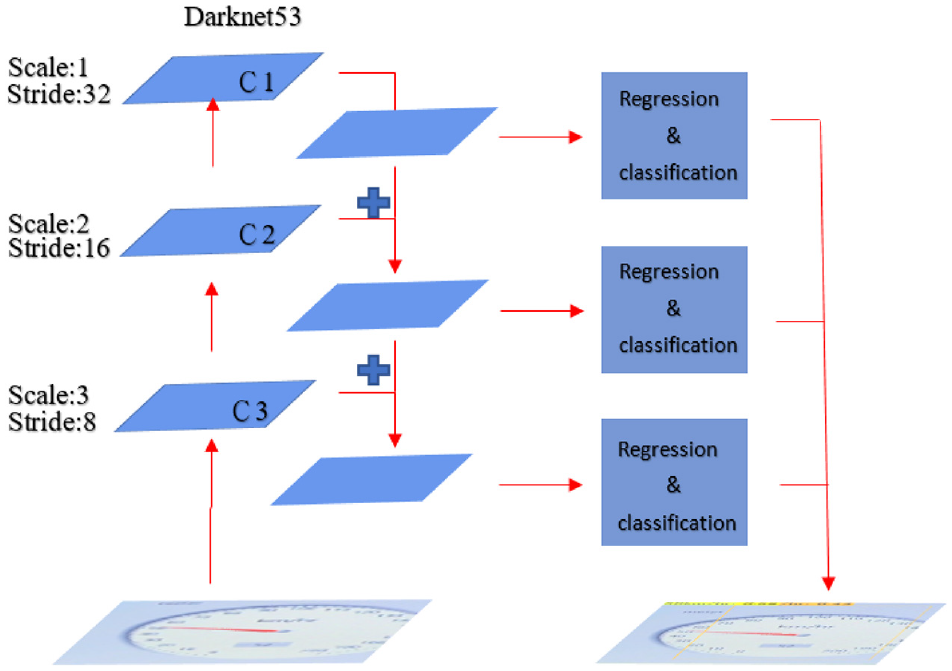
The architecture of YOLOv3, and C1~C3 refer to the feature layers.
The loss function (equation (1)) is defined as follows.
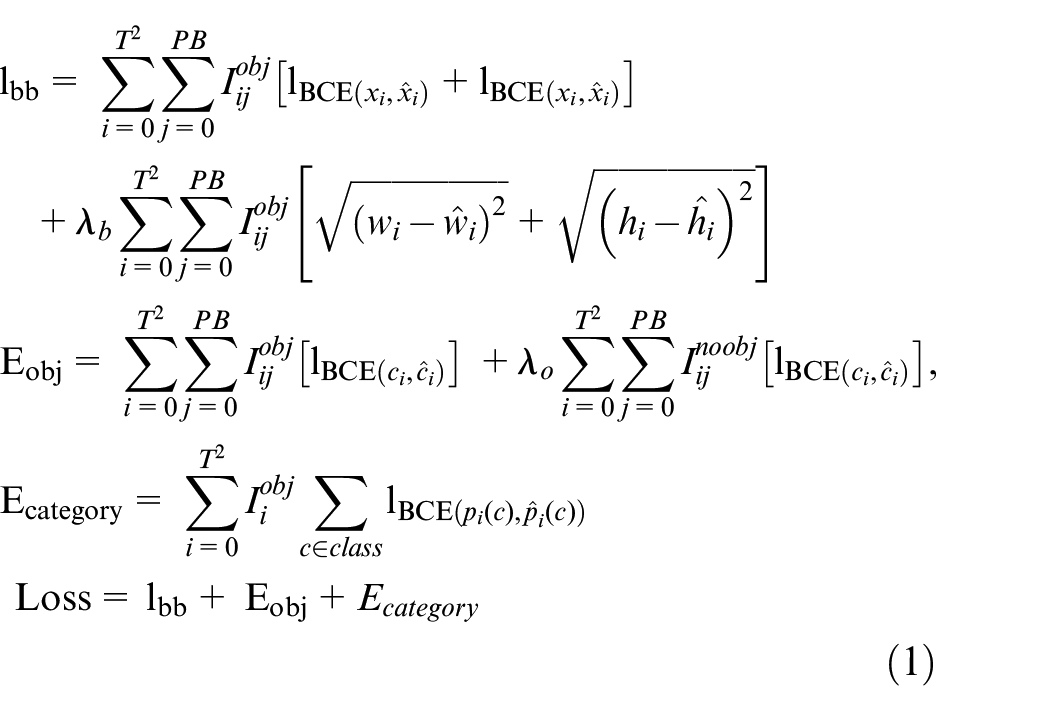

The
YOLOv4 deep learning network
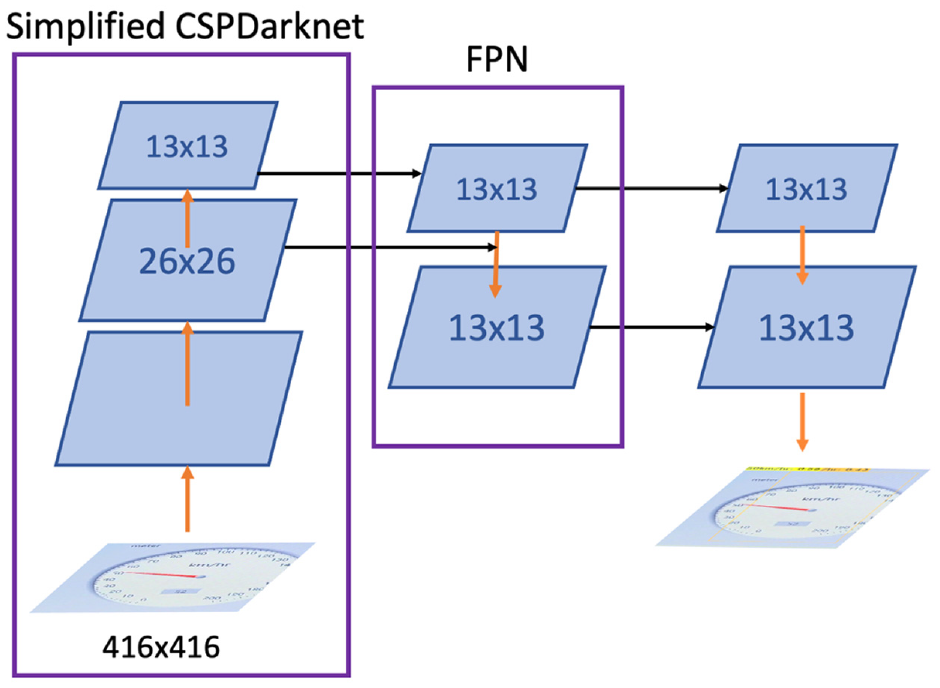
YOLOv4 developed by Bochkovskiy et al. 7 is a much-improved version in the YOLO series algorithms. The previous version, YOLOv3, has already done a great job of improving detection accuracy. Therefore, the network architecture of YOLOv4 is practically based on YOLOv3. The more distinctive difference between both versions is the backbone. Unlike YOLOv3 that uses DarkNet53 as the backbone, YOLOv4 uses the cross-stage partial (CSP) version. It enables YOLOv4 to reduce a large number of required calculations during the single forward propagation through the neural network. As a result, the Average Precision (AP) and FPS have increased by 10% and 12% on the MS COCO dataset, respectively.
YOLOv4 7 also obtains good detection results on a single GPU such as 1080 Ti and 2080 Ti and demonstrates more favorable overall performance. Besides, YOLOv4 is easier to obtain a high-accuracy model under a single GPU. The prediction time is similar to that of YOLOv3. The classic algorithm modules frequently used in deep learning models for design improvements were carefully selected and tested, and some modules were improved to realize a fast and accurate detector. The improvements were primarily related to the choice of backbone and the integration of several skills. CSPDarknet-53 7 was selected as the backbone network of the detector, as mentioned above. SPP block 8 was added to expand the acceptance flexibility of the model. In addition, the improved model, PANet, 7 has replaced FPN. As for the tricks, the detection modules most suitable for YOLOv4 and most often used in deep learning were selected, including Mish as the activation function and DropBlock as a regularization method. Furthermore, YOLOv4 uses a new data enhancement skill called Mosaic, 7 which expands data by stitching four images together. Several existing methods, including SAM, 7 PANet, 7 and cross-mini batch normalization 7 were employed to adapt YOLOv4 to training with a single GPU. Overall, the main structure of YOLOv4 comprises CSPDarknet-53, SPP, PANet, YOLOv3 Head, and Tricks, as displayed in Figure 2.
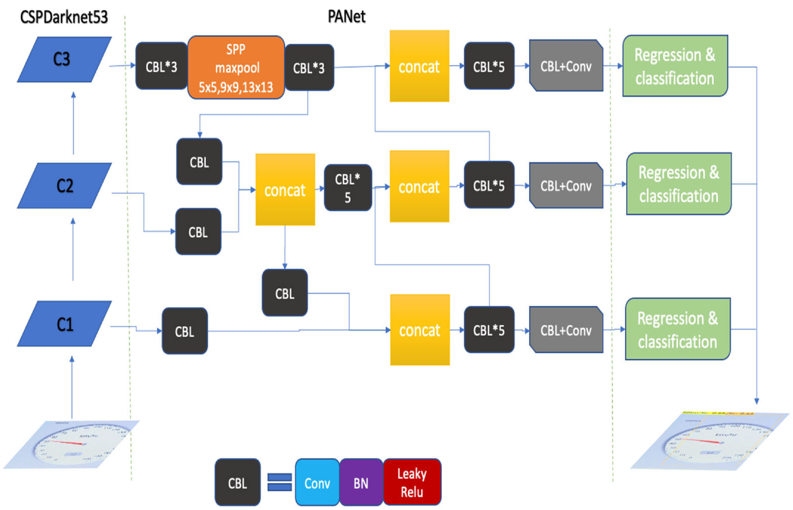
Structure of YOLOv4.
Compared with other outstanding object detectors, YOLOv4 possesses many advantages by conducting state-of-the-art modules. Through multiple experiments, YOLOv4 obtained an AP value of 43.5% on the MS COCO dataset, and achieved a real-time speed up to 65 FPS on the Tesla V100, gaining the title of the fastest and the most accurate detector among the YOLO series. Results can be viewed in Figure 3. Another outstanding feature of YOLOv4 is the detection at three different scales, which allows it to detect objects of various sizes. As a result, YOLOv4 detects better on small objects from a distance compared to other YOLO versions.
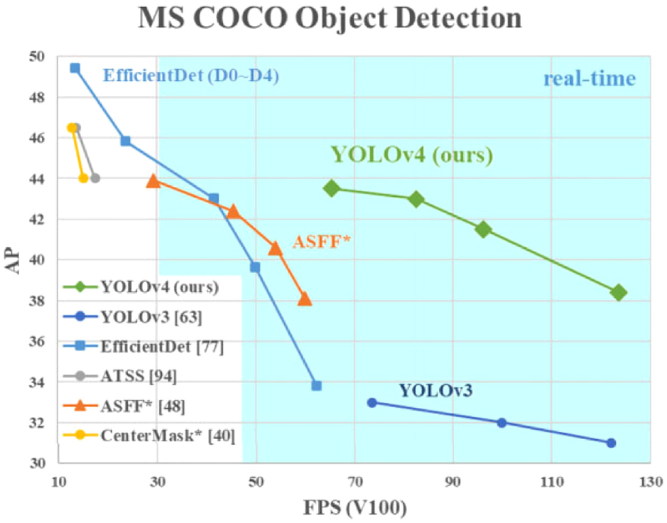
Comparison between YOLOv4 and other object detectors. 7
YOLOv4-tiny deep learning network
YOLOv4-tiny is a simplified version of YOLOv4. Although YOLOv4-tiny shares the same backbone structure as YOLOv4, which is CSPDarknet53, it has done some revisions to its residual calculation. YOLOv4-tiny replaces the originally adding with concatenating to assemble the previous feature extractions, leading to simpler calculations. Moreover, two CSP modules are subtracted from the original structure, leaving three modules to the task, which greatly reduces the number of calculations. As for the Neck of the neural network, YOLOv4-tiny eliminates the SPP and the PANet structure while reducing the output channel into two. Furthermore, YOLOv4-tiny chooses the Leaky ReLU as the activation function, comparing to YOLOv4’s activation function, Mish, which is relatively simpler. The number of filters that YOLOv4-tiny uses during convolution is also a lot less than YOLOv4. All of the modifications allow YOLOv4-tiny to attain faster execution and training speed (Figure 4).
Structure of YOLOv4-tiny.
Comparison with Faster R-CNN
A single CNN is a category of neural network in the deep learning field. It divides the input image into regions and predicts the bounding box along with the occurring probabilities of objects of interest in every region. Nonetheless, this leads to the overwhelming computation of a huge number of regions.
Hence the Region-Based Convolutional Neural Networks (R-CNN) is created. The proposed method extracts up to 2000 regions from the image and uses CNN as a feature extractor. The extracted features are subsequently fed into Support Vector Machine (SVM) to locate and classify the object. 9 However, R-CNN and the improved version, Fast R-CNN that acquires the selected regions after the input image is being fed to the CNN to generate the convolutional feature map, both use selective searching to obtain the proposed regions. It can be time-consuming and affect the performance of the network. Therefore, Faster R-CNN is brought up to solve the problem. Instead of using a selective searching algorithm to identify proposed regions, a separate network is deployed to achieve such a purpose. Experiment results show that Faster R-CNN is much faster than its predecessors, 10 so in this study, we’ll only compare YOLO with Faster R-CNN to find out the better between both.
Unlike the above two-stage deep learning network, YOLO, the single-stage detection, applies a single convolutional network to predict the class probability within each bounding box drawn in the input image’s grids. 11 It allows YOLO to finish its end-to-end detection performance at an incredible speed (45 frames/s), which is faster than any other deep learning network. 12 However, the downside of a single-stage deep learning network is its low accuracy compared to the R-CNN. Thus, YOLO has gone through different versions and has evolved into an outstanding model by enhancing its network structure and increasing anchor number.
YOLO and Faster R-CNN both have their pros and cons. On balance, our study aims to achieve real-time object detection. Hence, we select YOLO as our deep learning network.
Methods
Overview
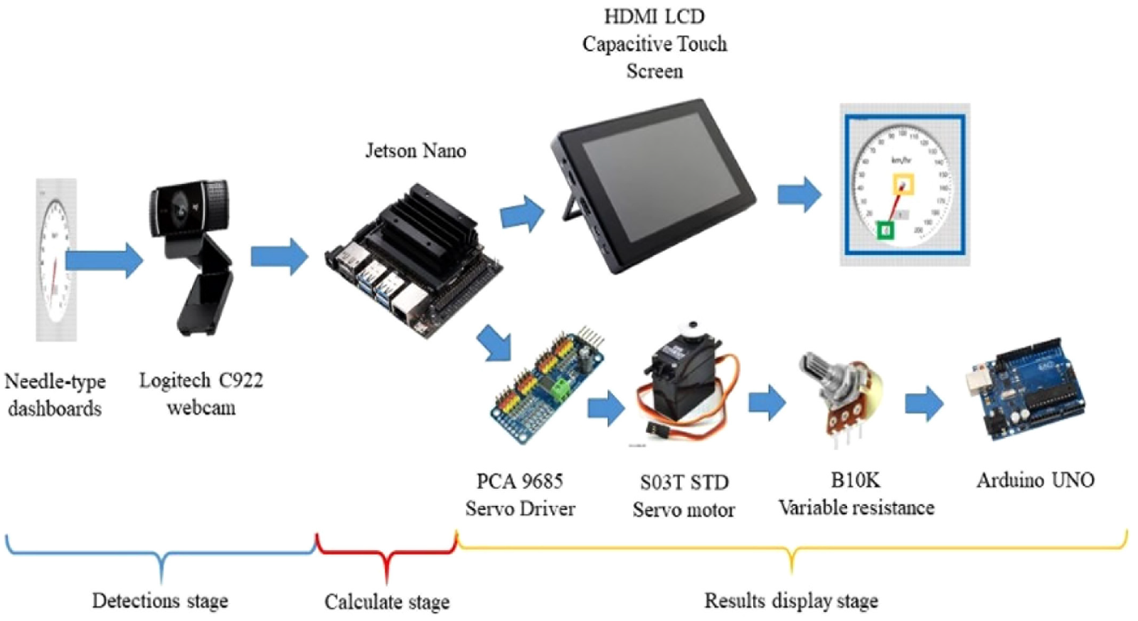
Figure 5 presents the flow chart of image sensing by YOLO based technique for the dashboard meter recognition. Following sections will detail the concept of design and how to manipulate and synthesis a new neural network for goal of this study.
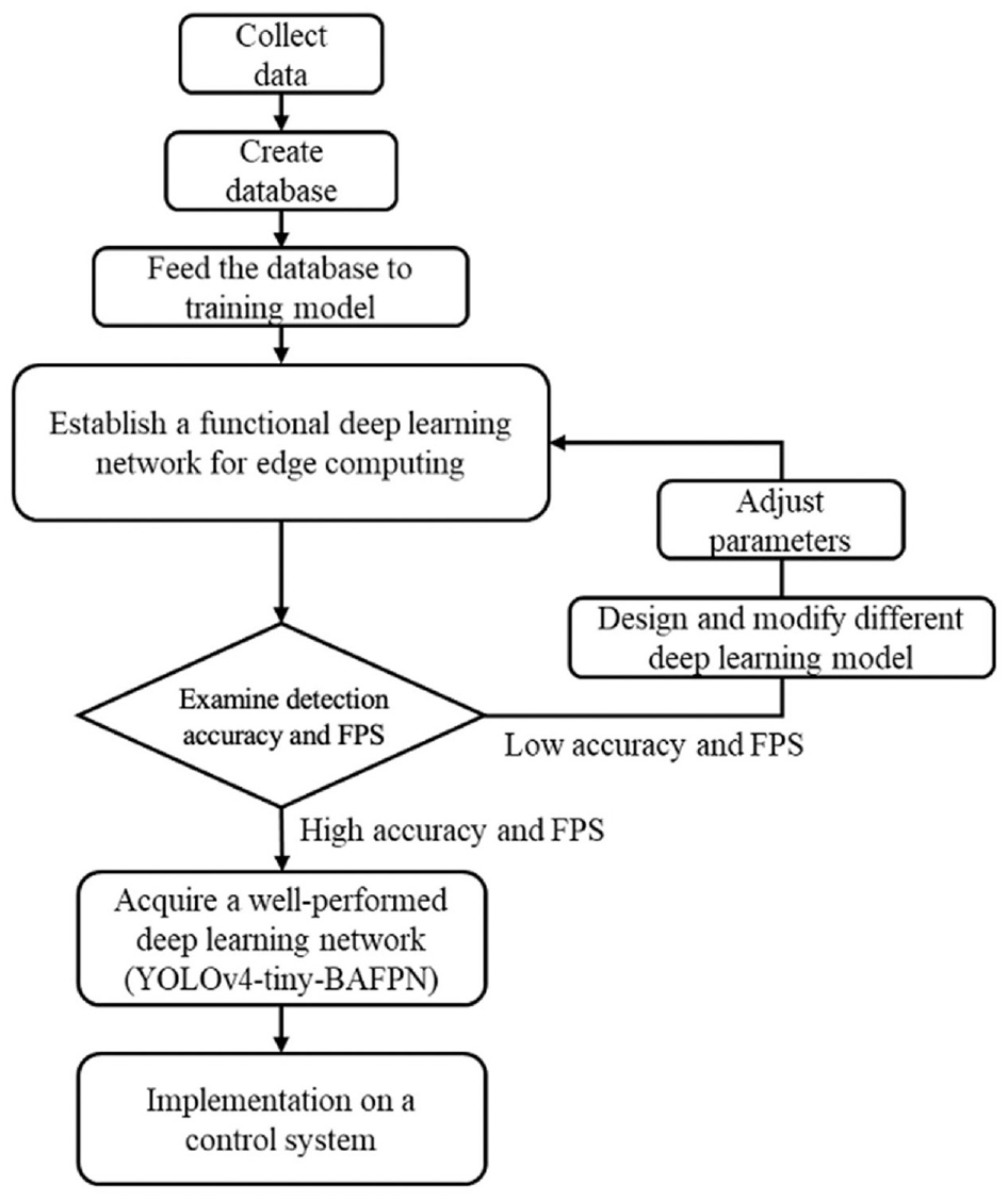
Flow chart for image sensing by YOLO based technique.
The CNN structure
When it comes to the CNN structure for deep learning network in this research, heuristically, YOLOv4 is the candidate, since it is one of the most accurate and fastest deep learning networks among those in the industry. However, throughout many experiments, we found out that it’s hard to process YOLOv4’s CNN structure on the NVIDIA Jetson Nano in real time implementation. Although the NVIDIA Jetson Nano contains high-performance GPUs and supports varieties of toolkits that help to process convolutional neural networks. But as YOLOv4’s neural network model is concerned, the FPS of which fails to meet the demand of FPS for imaging dashboard meter.
In replacement, YOLOv4-tiny turned to the candidate. Although YOLOv4-tiny has a great FPS value and can favor the requirement of real-time detection. Yet its accuracy is relatively worse and cannot fit in this conducting experiment. Initial test of the mAP of YOLOv4-tiny in our dataset is merely 53%. Therefore, we have to modify the Neck of YOLOv4-tiny to improve detection accuracy.
In this research, we added both the SPP and BAFPN into the Neck of YOLOv4-tiny as shown in Figure 6. The modified CNN model provides better accuracy than YOLOv4-tiny while being simpler than YOLOv4 and therefore can precisely detect objects on an edge-computer with higher FPS.
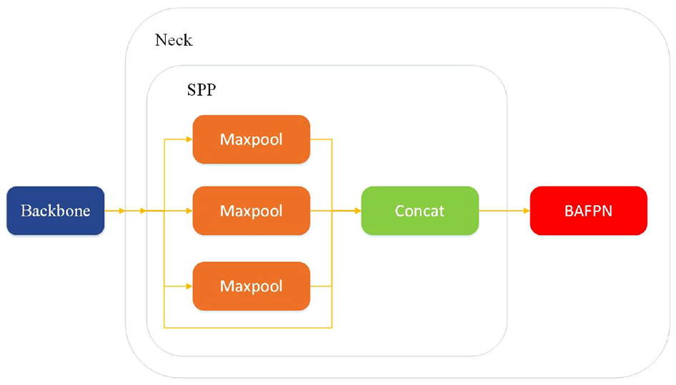
Illustration for the modified YOLOv4-tiny structure by adding the SPP and BAFPN within the Neck structure.
To elaborate, the reason we brought in the SPP is that it was a major breakthrough when the YOLO-based algorithm evolved from version 3 into version 4. Moreover, the SPP model was initially developed to complete the feature fusion with little calculation for the purpose of having high detection accuracy without losing too much detection. speed, so it is an essential structure if we need to increase the AP value of our CNN structure.
In most neural network models, they predict objects based on global features. The global features are indeed invariant. In other words, they contain fewer details from the input images. Thus, global features are poor in detecting datasets that have small variations between classes. Nevertheless, the local features are much different. The data in local features are much varied, which means that they are sensitive in detecting small differences between input images. Based on the concept, the FPN model is formed. The FPN model fuses global features with local features through upsampling. Also, the operations are independent of each other, so the features from both local and global can be retained.
Since the BAFPN model is based on the structure of FPN. It improves the connection between local features and global features. By fusing both of them, we can achieve an effective learning process. Some detailed structure of BAFPN is shown in Figure 7. Three different sizes of every image are drawn out from the backbone, to even out global features and local features. Through multiple upsampling, maxpooling, feature extraction, and adding, the CNN outputs the same image sizes as the input.
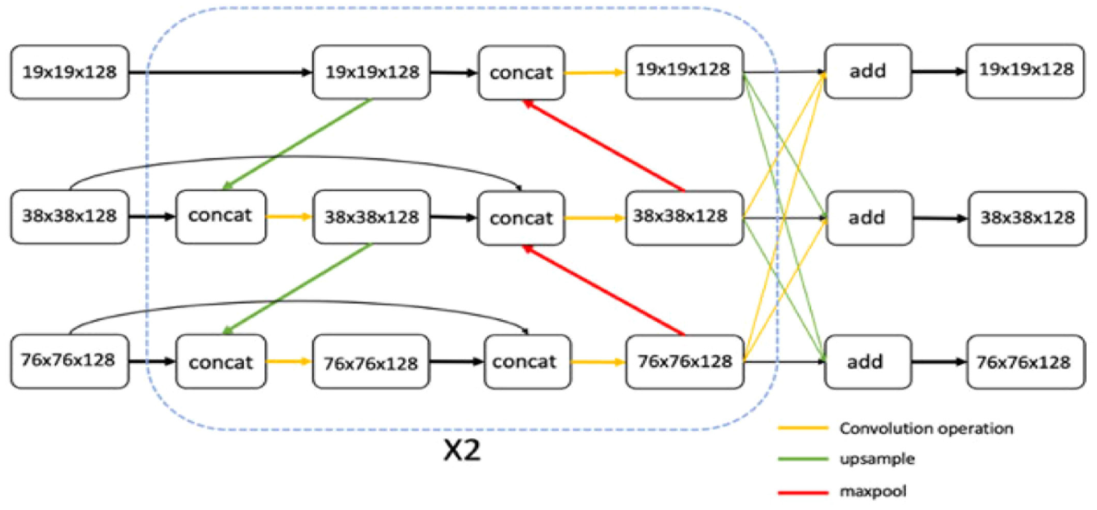
Illustration for the BAFPN.
Taguchi method for bettering Hyperparameters in CNN
After modifying the CNN structure, the image recognition results were still not satisfying. Therefore, adjusting hyperparameters to improve the prediction became the next phase. In YOLOv4, we can simply separate them into three parts, the net section, data augmentation, and optimizers. By experimenting with various combinations of hyperparameters to achieve the best performance is very time-consuming and pointless. Because the best combination of hyperparameters can vary from different datasets and the number of contained parameters is massive. Consequently, in this paper, the hyperparameters are adjusted according to the Taguchi method.
Taguchi method is an optimization method in quality engineering. Its method is to combine average output and average variability and form a single indication for determining the optimal objective function. Based on statistical theories, the Taguchi method was developed to improve the manufacturing process in product lines. And recently, it has proven to be effective for designing parameters in neural networks. 13
In this paper, we are looking for the best combination of hyperparameters that allows our CNN to achieve the highest mAP from our dataset. Therefore, Larger-the-best (LTB) is selected in our case. Besides, due to the numbers of factors, the L8 orthogonal array is chosen in this paper.
Factors and levels
To operate the Taguchi method, the first step is to seek appropriate factors, which are the variables in the experiment. In the YOLOv4-tiny-BAFPN, the hyperparameters of the training model are set to be the factors. Basically, the factors can be separated into three parts: net section, data augmentation, and optimizers.
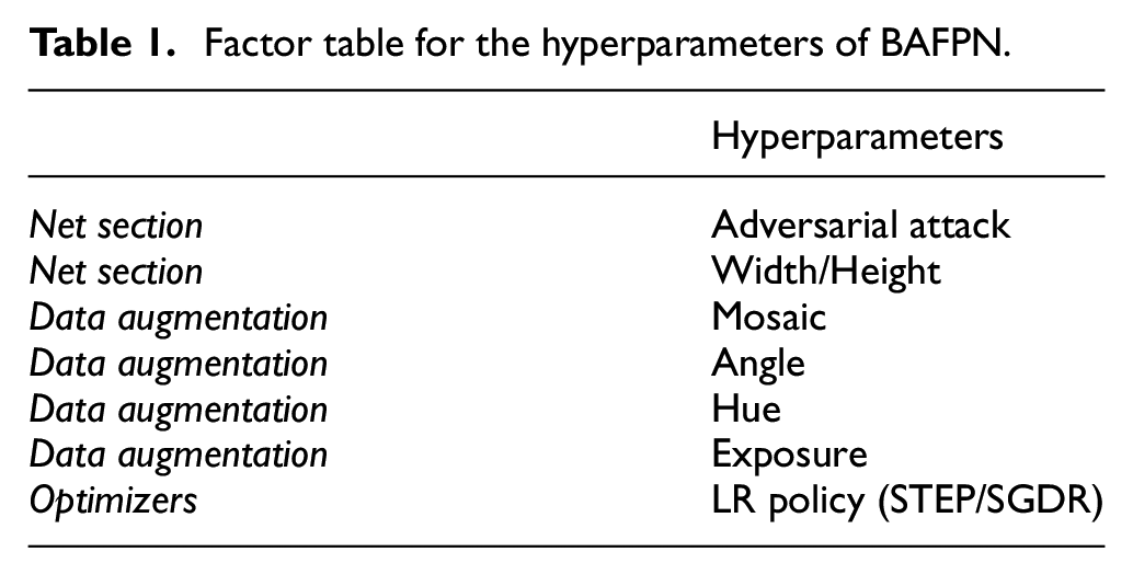
The hyperparameters in the net section are the factors that influence how images are sent into the training process. The hyperparameters in the data augmentation section are used to change the input images to improve the variety of images. Then, the hyperparameters of optimizers are associated with the learning rate, including the learning rate itself and its decreasing function. The hyperparameters chosen to be the factors in the Taguchi method are shown in Table 1.
Factor table for the hyperparameters of BAFPN.
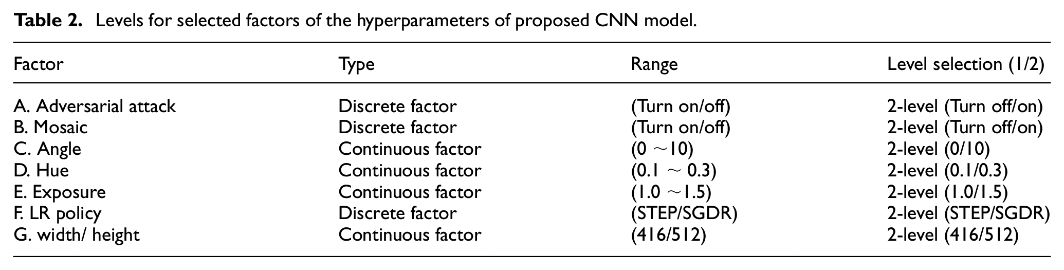
Levels are the choices for each factor. When configuring the level of each factor, we can divide factors into two types, continuous factors, and discrete factors. If the parameter is monotone, it can be classified as 2-level. However, if the parameter is not monotone it should be classified into different level according to its influence on the target value. Therefore, the Angle, Hue, and Exposure were selected. In addition, due to the limited calculating ability of NVIDIA Jetson Nano, the input network size cannot be over 512 × 512. Otherwise, the calculation will be too heavy to achieve real-time detection (Table 2).
Levels for selected factors of the hyperparameters of proposed CNN model.
Optimization
In this research, we hope to optimize the parameters to achieve better detection performance. Thus, average precision (AP) is a suitable index to show the ability of detection. AP is the area under the line on the recall and precision coordinates, while the mAP is the average of AP among all detection objects. They are the standard indexes that show the degree of accuracy.
S/N (signal-to-noise ratio) is a measurement in engineering. It was used to describe the relationship between the power of signal and background noise. Its definition can be written as equation (3).

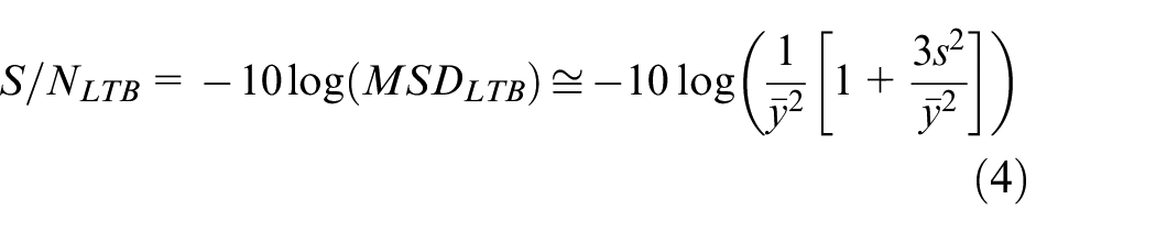
For the S/N ratio in the LTB case, the S/N ratio is described as equation (4)
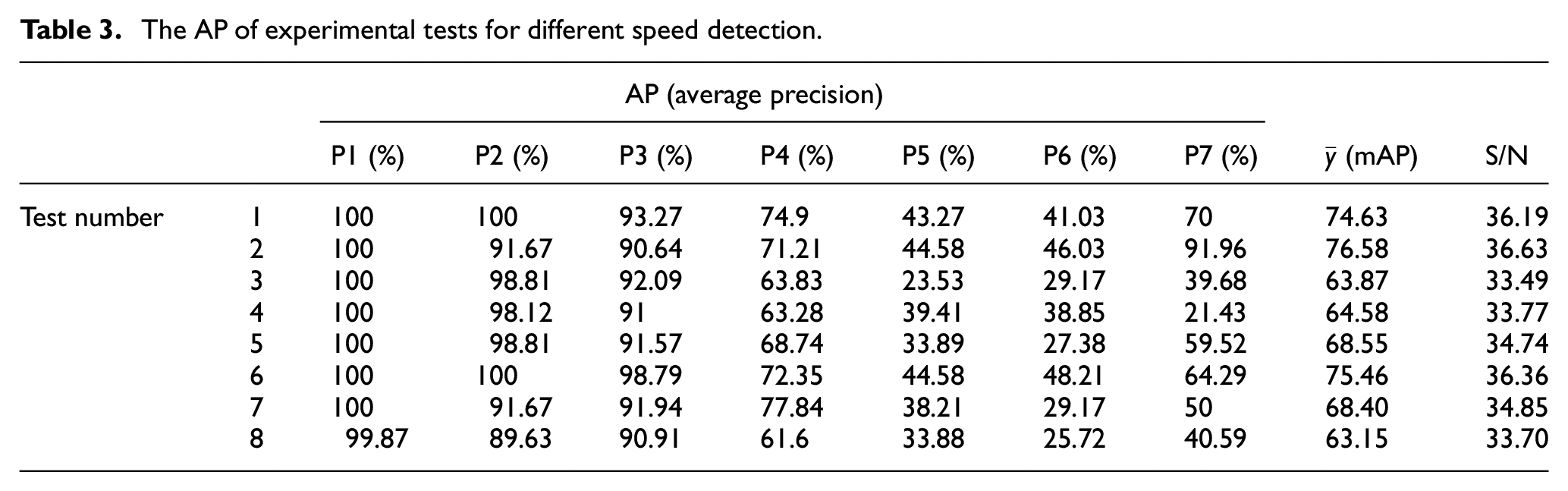
In Table 3, different object detection ranges by P1 (0 km/h), P2 (10 km/h), P3 (20 km/h), P4 (30 km/h), P5 (40 km/h), P6 (50 km/h), and P7 (60 km/h) are obtained for the AP, mAP, and the S/N, respectively.
The AP of experimental tests for different speed detection.
Rearrange the variability of S/N in each factor, the effect plot is shown below (Figure 8).
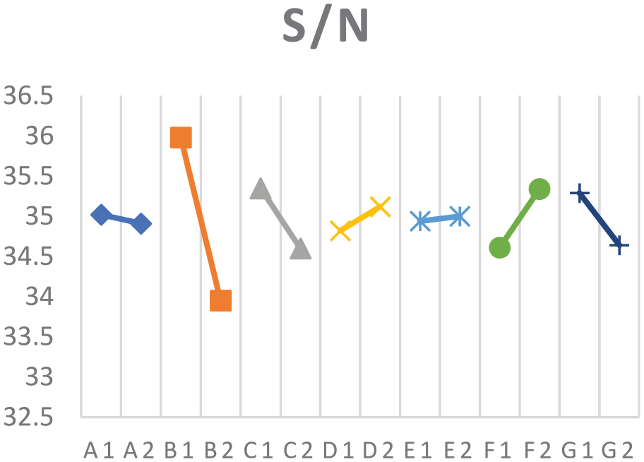
The effect plot of S/N for different factor.
In each factor, bigger S/N is our preference, which means the ability of detection in the different ranges is more stable and reliable. By analyzing Figure 8, we classified the factors that are influential to our dataset through the half rule, which is a common way to distinguish factors. Therefore, the choices for option 1 and option 2 for each factor are listed in Table 4. The optimized options that will provide higher S/N values.
Option of significant factors.
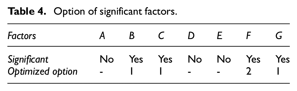
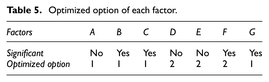
It is hard to make sure the optimized option of factor A, factor D, and factor E in Figure 8 because the changes on S/N in both levels are roughly equal. Under these circumstances, we can assure that these three factors contribute less in improving the ability of detection stability. Also, the performance in improving mAP in factor A, factor D, and factor E did not significant (Figure 9). Thus, these three factors should be determined by other indicators, such as detection speed. However, these three factors did not interfere with other elements, so we decided to set these three parameters as shown in Table 5 according to the slight change of their S/N and mAP.
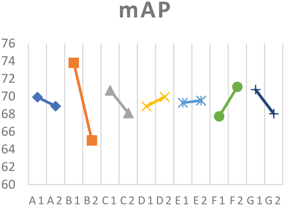
The effect plot of mAP.
Optimized option of each factor.
Verification
Before we confirm the result of the Taguchi method, we have to ascertain that there is no interaction between factors in this experiment for the reason that the statistical theories behind the Taguchi method are based on the independence between factors. In other words, only when there is no interaction between factors will make the optimization complete. Therefore, we have to prove the independence between factors exists.
Assume the independence between factors exists, the influence of each factor can be superimposed in mathematics. Based on the additive model, we can predict the S/Noptimal by the equation (15), and the result is shown in Table 6.
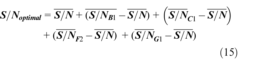
S/N value of optimal setting.
The predicted S/N and the S/N from the experiment have a pretty good consistency (the gap between the experimental result and predicted result is smaller than the 95% confidence interval), which means this result of experiment is reliable, and the effect of mutual influence between factors is small.
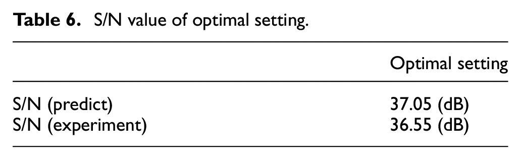
In addition, the verification of the Taguchi method is to ensure there is no error deviation before massive manufacture due to the fact that only a few samples are used to represent the whole dataset, and this will sometimes mislead experimental design. Thus, the verification is an important process in the Taguchi method. However, in our experiment, testing mAP originally contains massive samples because every mAP value was collected from over 100 images. This makes the results of our experiment more dependable. Figure 10 depicts the flow chart of the Taguchi method for bettering hyperparameters of proposed CNN structure.
Flow chart of the Taguchi method.
Experimentation
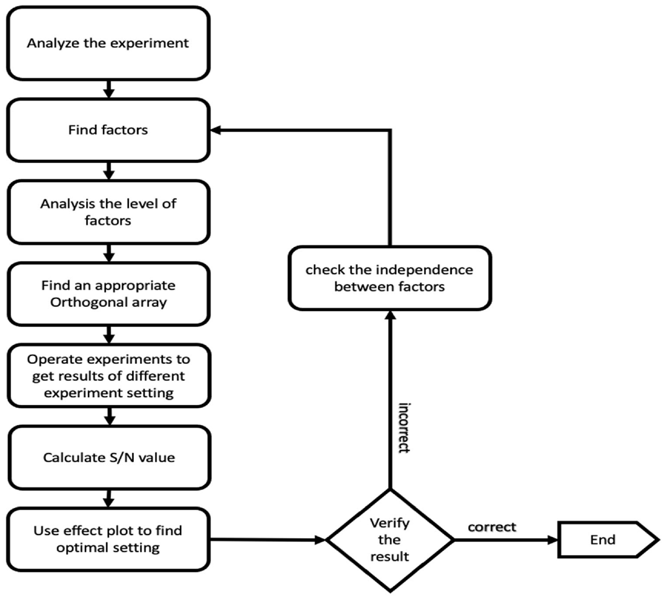
Focus on creating a fitted CNN structure for edge computers to process and determined the optimal hyperparameters via the Taguchi method is elaborated in above section. This has led to the creation of a trimmed deep learning network, YOLOv4-tiny-BAFPN. We would like to verify whether proposed trimmed deep learning network can be put into practice. Therefore, establishing an experiment based on the speed indication of a needle-type dashboard is conducted as follows. Since the aim is to design a system that can achieve error correction and self-control by approaching the input speed with visual recognition. Figure 11 demonstrates the feasibility and validation of the experiment process for the needle-type dashboards recognition. The experiment can be sorted into four stages, including data collecting, image recognition, signal processing, and mechatronics control, which will be introduced in the next section.
Experiment process for needle-type dashboards image recognition.
Data collecting
To achieve precise control of the pointer, recognition data is required. The current speed, the positions of the pointer’s end, and the center of the dashboard are all essential data. And therefore, we have established a database consists of the above-annotated data through labeling (Figure 12).
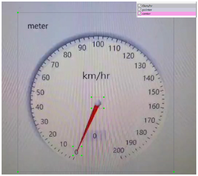
Demonstration for needle-type meter and data labeling.
Recognition
The Logitech C922 camera was employed to receive the dashboard’s display (Figure 13) for object detection dataset. And the acquired images will be transmitted to the Jetson Nano developer kit, which serves as our edge computer, and inputted for object detection. The YOLOv4-tiny-BAFPN deep learning network will conduct convolutional calculations and detect the “current speed,”“the pointer’s end,” and “the center of the dashboard.” Results will be displayed on the mobile screen and can be used for confirmation (Figure 14).
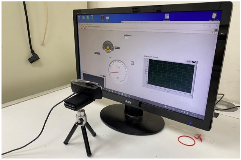
Illustration for image data of the dashboard from camera.
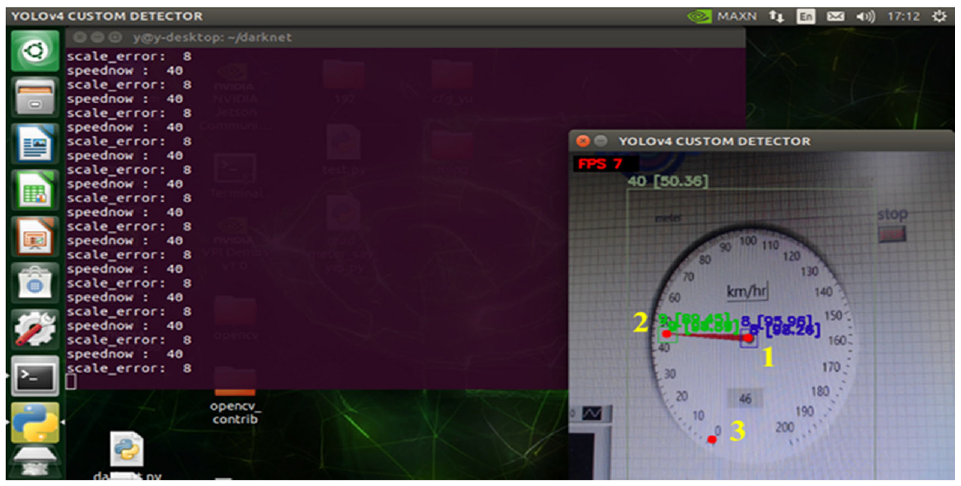
Picture of the system operating on NVIDIA Jetson Nano.
Processing
To actuate the pointer to automatically approach the input speed, PID control was adopted and classified it into two-stage control, which are “broad controlling” and “precise controlling.” During broad controlling, when the activated control action roaming to the desired speed, we considered the speed difference between the current speed and the desired speed as the input of the PID control. As for precise controlling, the angle difference between the current pointer’s position and the final speed scale was compensated by PID control. When the speed difference is relatively large and requires the pointer to ascend quickly, we apply the broad controlling. On the other hand, when we require the pointer to stabilize around the designated speed, precise controlling is put into use.
Controlling
The Inter-Integrated Circuit (I2C) bus-controlled driver PCA9685 that serves as a servo motor controller is connected to the Jetson Nano developer kit. By utilizing the PID’s speed gain calculations, a servo motor (S03T-STD) was controlled to output voltage variations through a 10 kΩ variable resistance and to actuate the LabVIEW dashboard’s pointer with the servo motor, as shown in Figure 15.
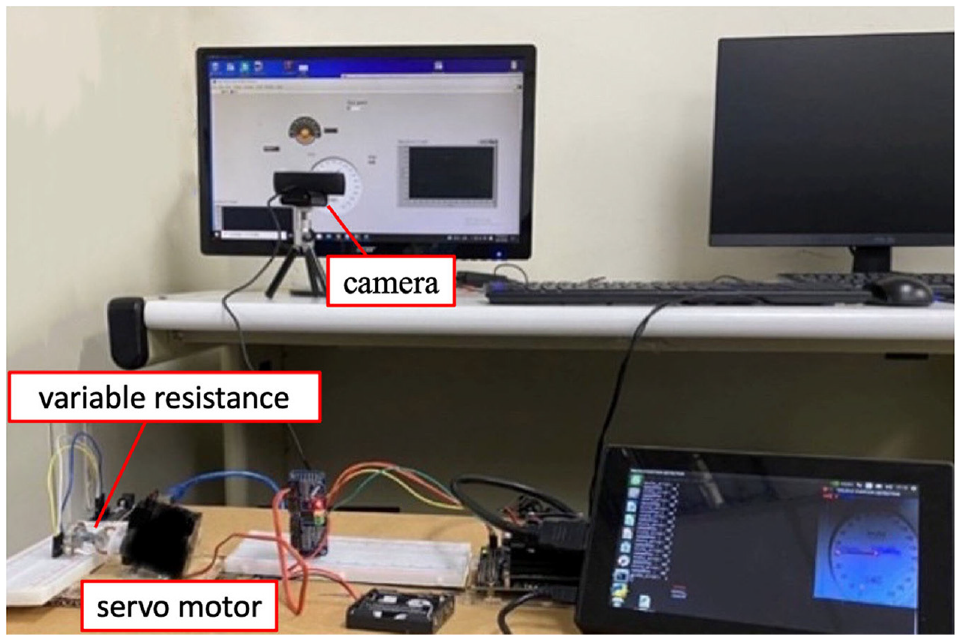
Picture of the experiment setup for camera imaging system (top) with control actuation apparatus (bottom).
Experimental components
Jetson Nano developer kit
The NVIDIA Jetson series is a deep learning network processing platform, designed for embedded systems. And the Jetson Nano is stated as the smallest device among the series while it provides powerful GPUs, which make it suitable in implementing CNN and real-time detection. In the proposed experiment, we have used the Jetson Nano developer kit as the main processer of the YOLOv4-tiny-BAFPN and programed it with Python 3.6.
PCA 9685 breakout board
The PCA 9685 is a 16-channel servo motor controller with an I2C bus interface, which is capable of driving Pulse Width Modulation (PWM). Every channel onboard can be programed independently. During the verification experiment, the Jetson Nano developer kit will output a controlling signal via I2C to the PCA 9685 PWM driver.
S03T STD servo motor
By integrating control loops and essential feedback, the servo motor can adjust itself to accomplish rotating and revolution speed with 16–23 ms cycle time under 4.8–6 V DC.
LabVIEW needle-type dashboard design
The dashboard interface in the experiment was designed in the graphic control software, LabVIEW, which includes the virtual dashboard, the voltage indicator, and a waveform graph generator to depict the system’s output. As for how fast the pointer maneuvers is controlled by the output voltage from the 10 kΩ variable resistance, where an Arduino UNO board was connected to the LabVIEW program. Besides, the servo motor is attached to the variable resistance, they share the same rotating angle. In other words, the servo motor controls the ascent of the dashboard.
PID control
System overview
The system takes the speed recognition of the needle-type dashboard as input and subtracts it from the final speed to generate an error value. According to the compensated PID signal (equation (16)), the error value can be used to generate the output U, which will be sent continuously to the operating closed-loop system, producing a new error correspondingly on a cycle basis. In this case, the speed difference between the final speed and the currently recognized speed is creating the speed gain, which is signified as the value U, and adding to the current speed to implement PID control. Whether the speed gain is a positive or a negative value, it represents the amount of speed the system needs to increase, in order to have less response time and more stability while reaching the desired level. The newly generated speed is yet again being recognized by our deep learning network and considered as the next cycle input. The above process runs repeatedly to achieve an optimum response. As for how the needle in the dashboard maneuvers to indicate the new speed will be discussed in the next section (Figure 16).
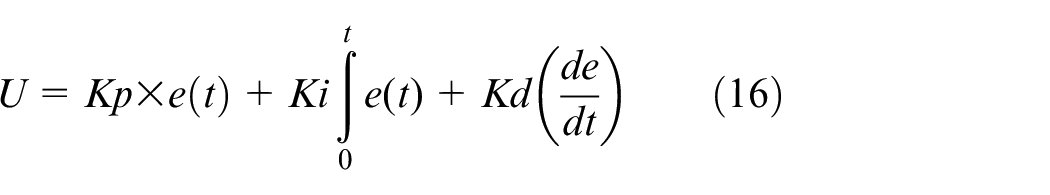
Control block diagram of the PID control for a single servo motor with finger pointer.
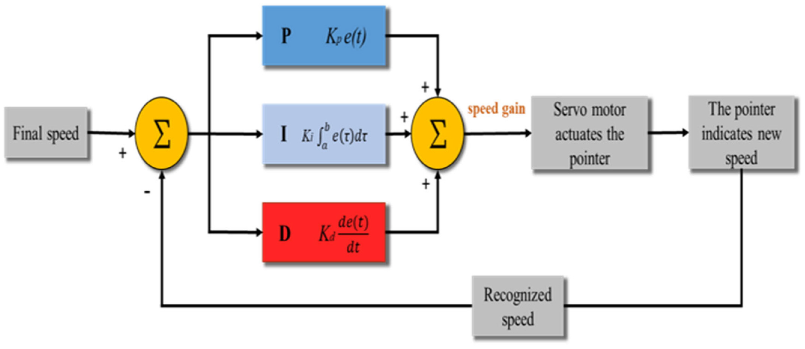
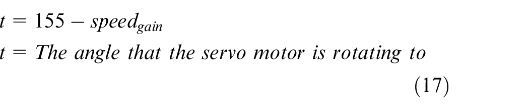
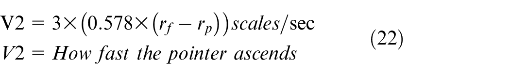
We have converted the speed gain into how much angle the servo motor will be rotating (equation (17)), which further determines how fast the pointer is going to ascend. Since the dashboard’s pointer is designed to maneuver 3 scales per second with the input of 1 speed gain. The ascending speed would be 3 times the output speed gain (equation (18)). In addition, the speed gain from the beginning should be the largest because it possesses the greatest error value when subtracting from the final speed. The rotating angle should also be at its greatest, causing the pointer to rotate substantially and rapidly. When approaching the designated speed, the pointer gradually slows down and finally reciprocates near the final speed.
Tuning demonstrations
PID controller is widely used in the industry because it combines all three types of control methods, which can greatly improve the controlling effect and are compatible with many systems. It’s usually difficult to find the best combination of the three control parameters and it sometimes takes experience to design a good PID controller. However, throughout many experiments, we have successfully acquired suitable Kp, Ki, Kd values by manually tuning based on the results. First, we only tuned Kp as 0.2 and set the other parameters to zero to see the effect with only proportional control. In Figure 17, with the final speed setting as 47 km/h, the graph shows that there are still steady-state errors occurring, which means the output cannot arrive at the designated speed.
Final speed set at 47 km/h, Kp = 0.2, Ki = 0, Kd = 0.
Consequently, the Ki value was increased to 0.2 as well. From Figure 18(a), we can see that the system’s output did reach the final speed, but the transient response still oscillated at a large range. Then set the Kd value to 0.1 as to offset the error. In Figure 18(b), the transient response performs a lot better compared to Figure 18(a).
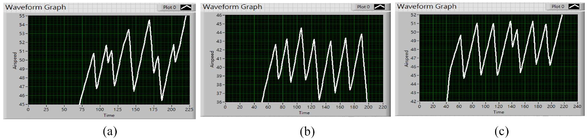
Final speed set at 47 km/h, for steady state compensation: (a) Kp = 0.2, Ki = 0.2, Kd = 0, (b) Kp = 0.2, Ki = 0.2, and Kd = 0.1, and (c) Kp = 0.2, Ki = 0.6, Kd = 0.1.
However, having increased the Kd value causes the output to fail to reach the designated level again due to the damping effect. As a result, we increased the Ki value by 0.4, and the output performance can be viewed in Figure 18(c). The graph reflects that the pointer did not only reach the final speed with a lot less rise time compared to Figure 17 but also reciprocated in a small range near the final speed, which indicates that these three PID parameters are suitable for our system to conduct the PID control. And therefore, we have successfully established a self-corrected system centering PID control with Kp as 0.2, Ki as 0.6, and Kd as 0.1 to actuate our pointer to reach the final speed more quickly while reducing the steady-state error. From Figure 19, with the final speed at 47 km/h, the system maneuvers quickly at the beginning, then tends to slow down when it’s close to 47 km/h, and eventually reaches a steady state. The result shows that PID control can indeed contribute a great controlling effect to our system’s response. Nevertheless, it still has room for improvements in terms of precise control. Though the compensation and the damping from the integral and derivative control restrain the system’s output from stabilizing at the final speed due to the low servo motor’s dynamic response. From Figure 18(c), we can observe that with the final speed established at 47 km/h, the pointer reciprocates between 45 and 51 km/h. The error value can still be reduced. Taking that into account, we have come up with a solution using only proportional control combines with angle recognition.
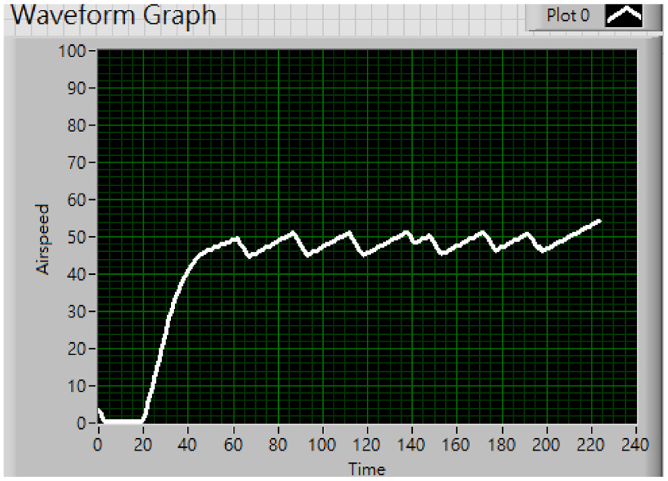
Final speed at 47 km/h.
Proportional control using angle recognition
Figure 20 presents the flow chart of the proposed control method. From Figure 14 we can see that the three red dots, 1, 2, 3, represents the position of the dashboard’s center, the pointer’s end, and the 0 km/h scale through object detection respectively.
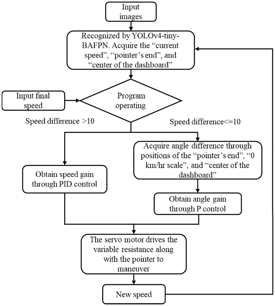
Flow chart for autopilot speed control based on YOLOv4-tiny BAFPN and PID controller.
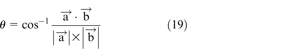
With the two vectors acquired, we can calculate how much angle the pointer has rotated by adopting the inner product (equation (19)).
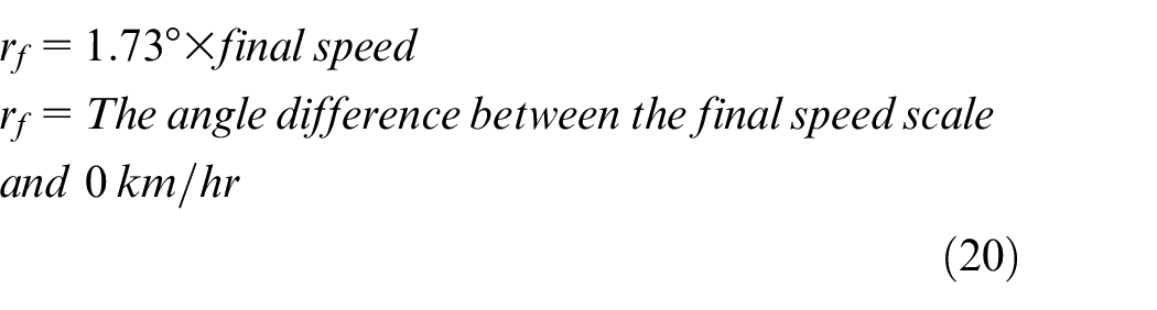
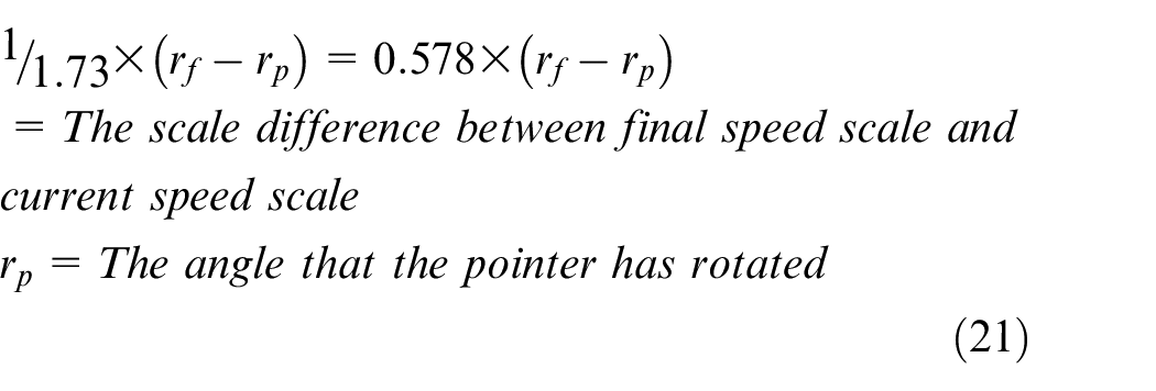
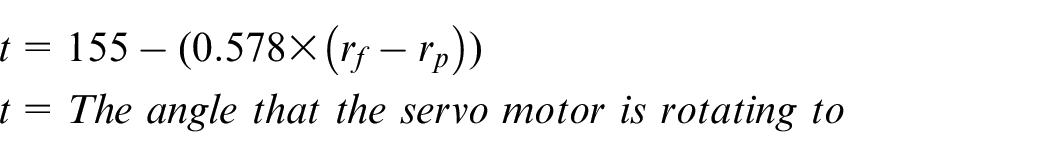
Having explained how the angle data is obtained, we can proceed to describe the controlling process using angle data. Throughout explicit measurement, we found out that the angle difference between every scale on the dashboard is approximately 1.73°. Therefore, we first obtained the angle difference between the final speed scale and the 0 km/h scale (equation (20)). Followed by the angle that the pointer has rotated. Lastly, the subtraction between both angles can indicate how much angle the pointer still needs to rotate to arrive at the final speed. We then utilized the angle data to conduct proportional control over how much angle the motor needs to rotate with the proportional gain of 0.578 (equation (21)). As mentioned in the previous chapter, the angle data can further determine the maneuvering speed of the pointer (equation (22)).
Results
Detection result
Our dataset contains three different dashboards captured from different angles. In total, we have collected 474 images for training and have labeled speed indication, the center of the dashboard, and the pointer’s end in each image with its class, center coordinates, width, and height. The speed interval ranges from 0 to 60 km/h, in the unit of 10 km/h. The detection process on the Nvidia Jetson nano screen is displayed in Figure 21.
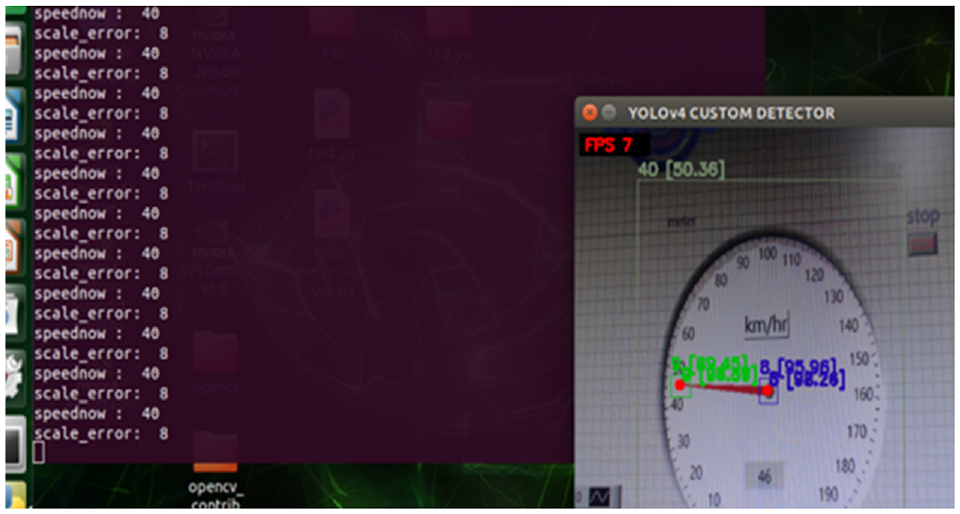
Detection process on the Nvidia Jetson nano screen.
The following demonstrates the training results from our modified CNN structure. The hyperparameters that were not adjusted in the Taguchi method were set as default values when training, with the number of 0.01, 4000, 0.0005, 64, 32 and 0.949 for the weight, training steps, weight decay, batch size, subdivision, and momentum respectively.
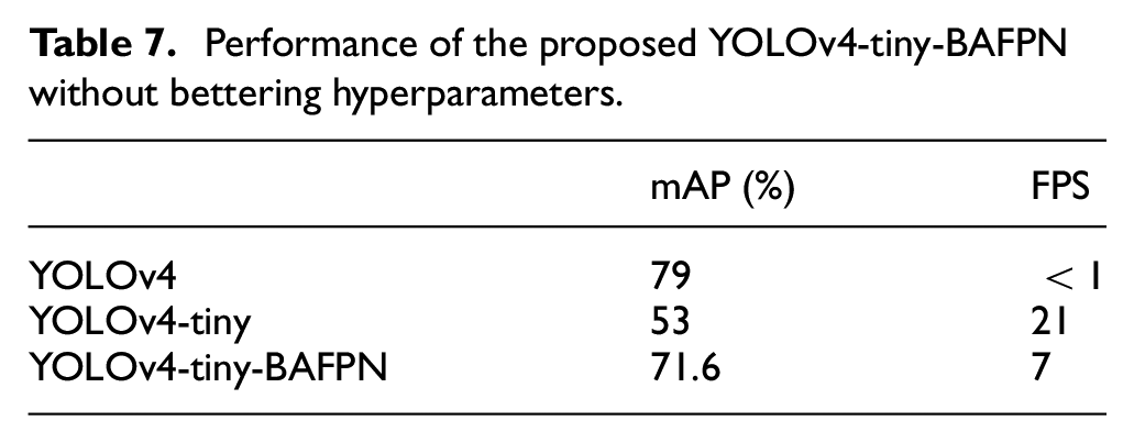
In our previous test, the performance of YOLOv4 on the Nvidia Jetson Nano can reach 79% mAP, but the performance of FPS is less than 1. This result was not good enough to achieve the improvement for future real-time detection. Nevertheless, using YOLOv4-tiny has the potentiality to meet the requirement for real-time detection. However, the mAP should be not good enough. Therefore, without changing the hardware device, we propose to improve the FPS while maintaining accuracy by modifying the neural network architecture of YOLOv4-tiny. Specifically, the structure we modified is the neck part of YOLOv4-tiny. As proposed, we have changed the neck structure by fusing in SPP, and BAFPN structure. Since the SPP structure improved the accuracy without costing a heavy burden to the whole structure. In addition, the BAFPN improved the ability to detect multiple objects at the same time and strengthened the performance of the whole structure by fusing local features and global features. By these changes, the modified CNN structure, YOLOv4-tiny-BAFPN, not only shows a good mAP compared to YOLOv4-tiny but also excels in detection speed compared to YOLOv4. This result successfully conforms to our original purpose (Table 7).
Performance of the proposed YOLOv4-tiny-BAFPN without bettering hyperparameters.
To optimize our deep learning network, we applied the Taguchi method to adjust hyperparameters, which can ameliorate detection accuracy without sacrificing detection speed. According to the Taguchi method, by using the provided orthogonal array, we can calculate the S/N and average value of each option. These two elements can be the determining index, creating an optimal parameters combination. The Taguchi method allows us to acquire the same result as those having gone through a time-consuming process of trial and error.
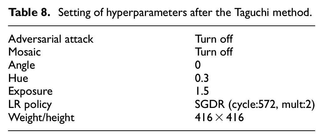
Using the L9 orthogonal array, we have conducted nine training processes based on different hyperparameters. As a result, we acquired a set of optimal hyperparameters from the analysis of the S/N and average value, see Table 8.
Setting of hyperparameters after the Taguchi method.
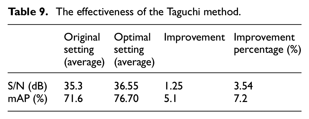
Repeatedly conducting three experiments under the best factor level combination (A1B1C1D2E2F2G1) for validation, we obtained an average value of S/N and mAP in Table 9. After adjustments, the S/N increases by 1.25 (dB), and the mAP increases by 7.2% compared to the default hyperparameters.
The effectiveness of the Taguchi method.
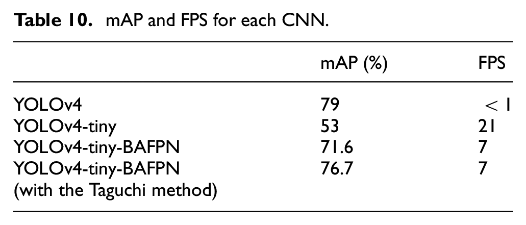
Combining the above approaches, the YOLOv4-tiny-BAFPN has almost the same accuracy as the YOLOv4 but is 7 times faster according to the FPS, which helps it run smoothly on the NVIDIA Jetson Nano (Table 10).
mAP and FPS for each CNN.
Controlling effect
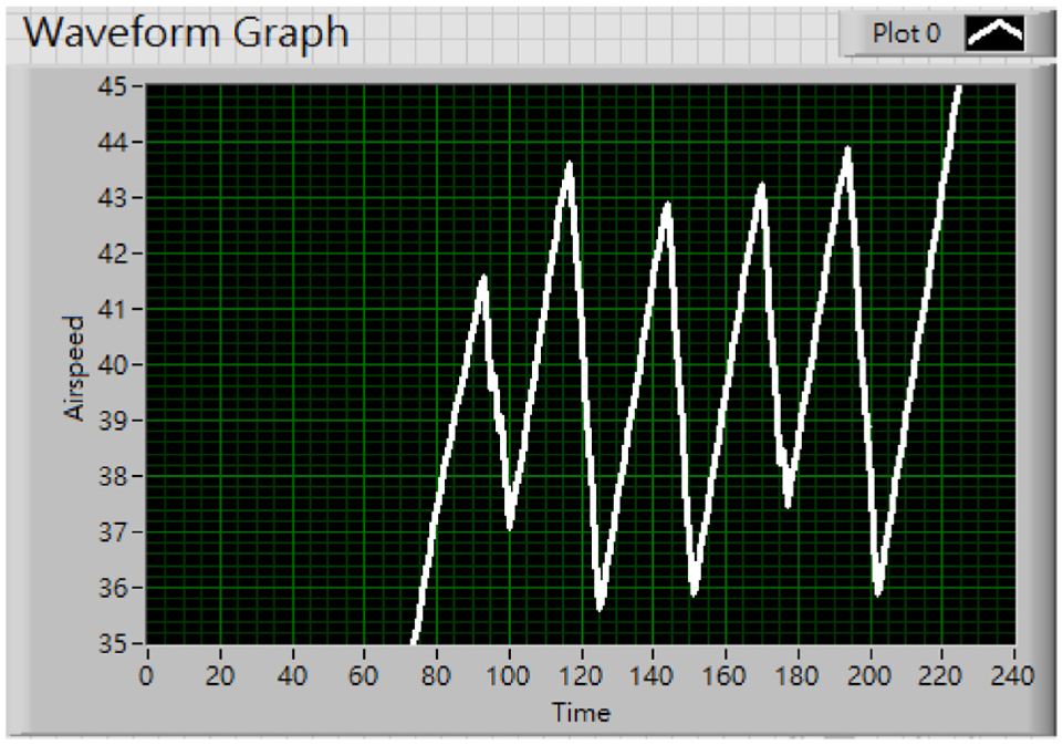
This section will be demonstrated how well the pointer maneuvers when adopting the proposed control method in Figure 20. We experimented with three different target speeds, which are 33, 47, and 55 km/h, respectively.
The above graphs Figures 22 to 24, all show that upon reaching the designated speed, the pointer reciprocates within an acceptable range, which has proven the proposed method to be effective in terms of stabilizing the pointer.
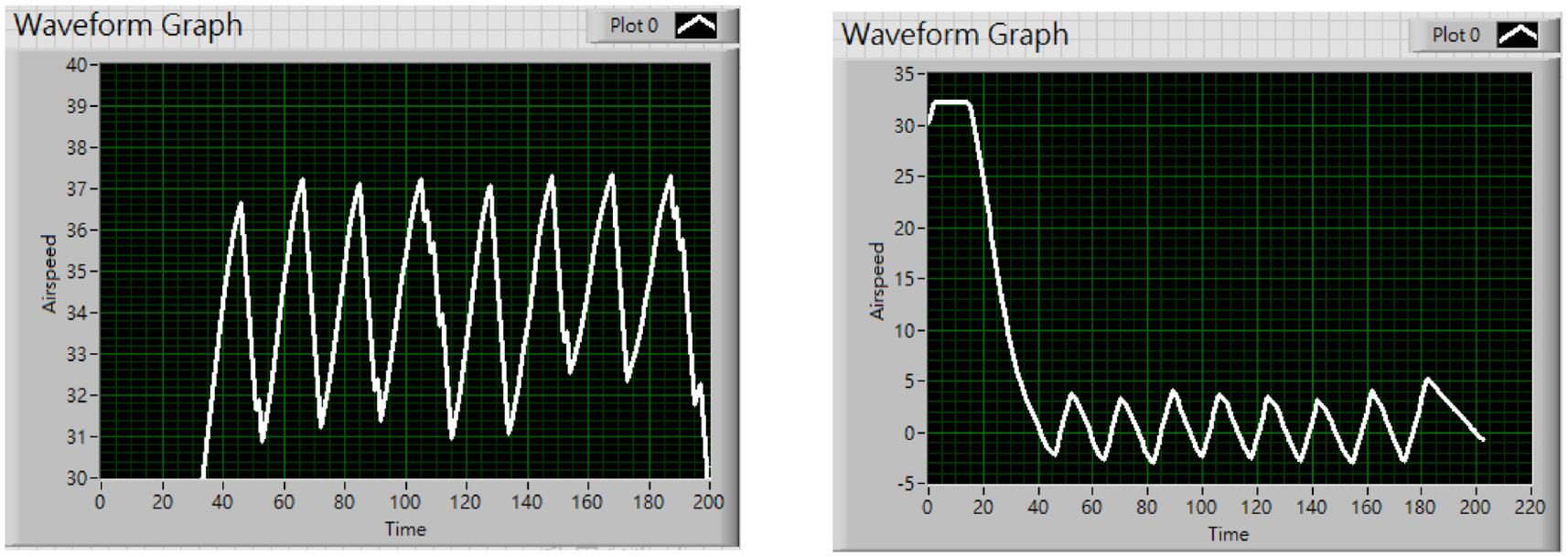
The final speed set at 33 km/h and its error value within the whole process.
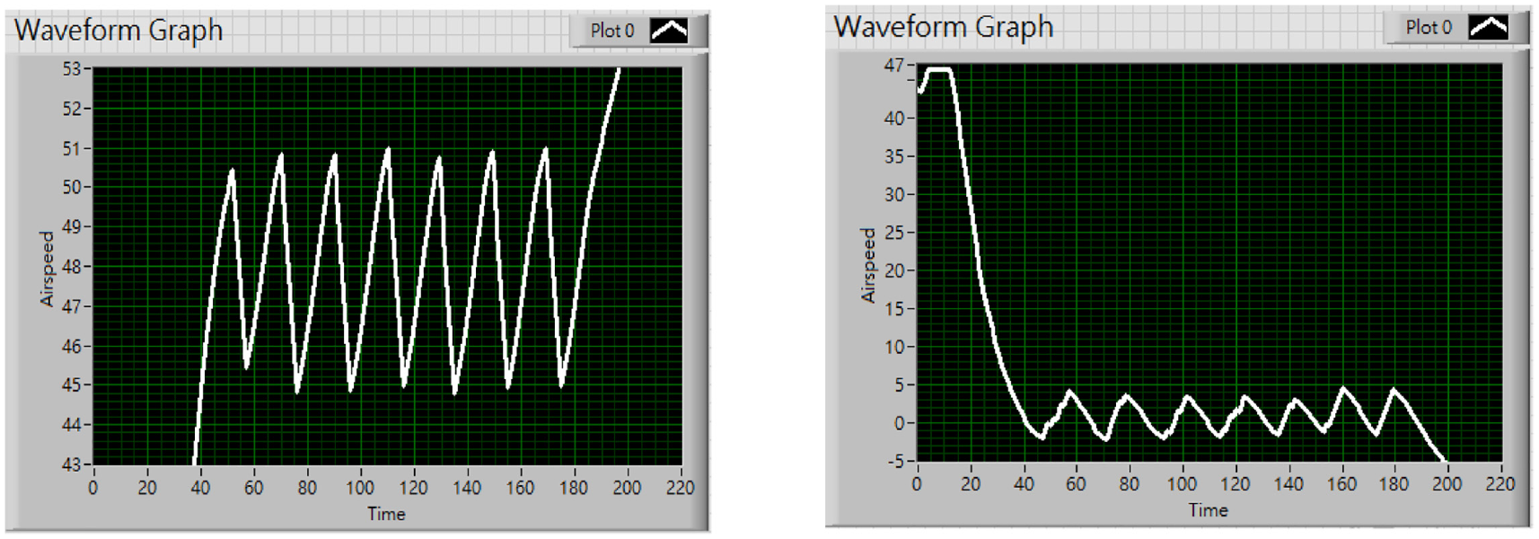
The final speed set at 47 km/h and its error value within the whole process.
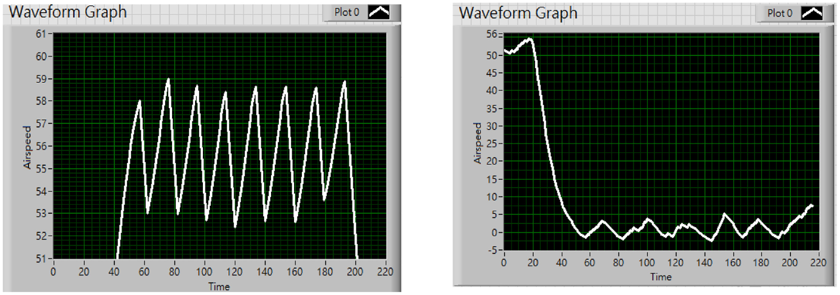
The final speed set at 55 km/h and its error value within the whole process.
By subtracting the current speed from the final speed, the error value is immediately obtained and displayed onto the graph. The graphs above demonstrate that the error value has the tendency to decrease while the pointer approaches the final speed. Additionally, from the error value plot above, it is clear that the steady-state error value won’t exceed the value 5. It shows affirmation toward the proposed control method concerning error correction.
As mentioned in section 3.1, the speed interval ranges from 0 to 60 km/h, in the unit of 10 km/h. This may lead to an overly large gap in detection. On that behalf, the proposed control method that involves angle recognition can easily improve the situation. Meanwhile, this approach also has a better performance compared to the method that only contains PID control (Figure 25).
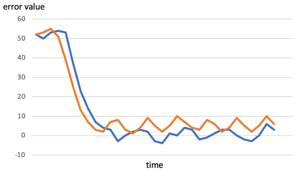
Comparison between conducting the proposed method (blue curve) and merely PID (orange curve) with the final speed at 55 km/h.
Conclusion
In this paper, a new YOLOv4-tiny-SPP+BAFPN deep learning model on needle-type dashboard recognition and a simple closed loop control system for autopilot maneuvering system is developed and demonstrated successfully. A new YOLOv4-tiny-SPP+BAFPN structure is created. We create a new YOLOv4-tiny structure by fusing SPP adopted from YOLOv4’s SPP structure and changed the FPN of YOLOv4-tiny by BAFPN structure. Adding the SPP structure improves the accuracy without costing a heavy burden to the whole structure. In addition, including the BAFPN structure improves the ability to detect multiple objects at the same time and strengthened the performance of the whole structure by fusing local features and global features. A Jetson Nano edge-computing feedback control system consists of a motor actuation and visual object detection web camera was developed. Based on the Taguchi method, adjustment of the hyperparameters was deployed successfully for the purpose of higher mAP and FPS. The object detection result of YOLOv4-tiny-BAFPN on needle-type dashboard integrated with the adjusted hyperparameters and feedback controller complied with the goal for autopilot expectations.
This paper also has great potential to be extended. We hope to apply object detection to receive all the other data displayed on different gages within the cockpit, including air pressure, temperature, flight attitude. Then, process the measured data through an advanced deep learning network and precisely control multiple sophisticated actuators to operate the aircraft. In conclusion, according to the result of this paper, it is possible to install a non-invasive system that automatically controls the aircraft such as to achieve autopilot in a variety of maneuvering systems.
Footnotes
Declaration of conflicting interests
The author(s) declared no potential conflicts of interest with respect to the research, authorship, and/or publication of this article.
Funding
The author(s) disclosed receipt of the following financial support for the research, authorship, and/or publication of this article: The authors thank the Ministry of Science and Technology for financially supporting this research under Grant MOST 106-2221-E-018-013MY2 in part and MOST 110-2623-E-005-001 and MOST 111-2623-E-005-003.