
Abstract
Due to the construction of ultra-high voltage transmission lines, the lines will inevitably pass through residential areas. The power frequency magnetic field created by transmission lines will affect the location and design of transmission lines, as well as people’s health. In this paper, the intelligent optimization algorithm is used to optimize the Simulation Current Method (SCM) and study the magnetic field distribution under the transmission line. Firstly, the actual three-dimensional shape of the transmission line is considered in this optimized simulation current method (OSCM). Secondly, we combined the magnetic position error with the magnetic field error to construct the fitness function, and we used the algorithm to optimize position and number of simulated currents. Finally, the finite element method (FEM) is used to verify the calculation results. We calculate a 500 kV 3-D transmission line model and verify that the optimized SCM can reduce the calculation effort and ensure the accuracy of the calculation. In addition, the OSCM solves the problem that the number and location of the simulated current can only be determined empirically. On the one hand, the actual physical shape of the transmission line is considered, which makes the calculation precision higher; on the other hand, the calculation time is much lower than that of FEM. At the same time, it provides a theoretical basis for the magnetic field distribution of transmission lines and has a theoretical guiding significance for the construction of high-voltage transmission lines.
Keywords
Introduction
With the rapid economic growth and increasing power demand, the ultra-high voltage transmission lines are under continuous construction. The voltage level and current of the lines are also constantly improving. As the planning and development of the power grid are not in line with the pace of urbanization, high-voltage and high-current transmission lines inevitably pass through small towns with dense populations. People who live under high-voltage power transmission lines for a long time will be affected by the electromagnetic fields generated by the power transmission lines, which will affect the blood circulation system, nervous system and other physiological functions.1–3 The effects of power frequency electromagnetic fields are very slow and take a long time to manifest. So, they have been ignored for a long time. With the enhancement of people’s health awareness, relevant departments are concerned about the impact on residents living near transmission lines for a long time.4–7 The location and design of transmission lines should consider the health of residents. Therefore, the study on the distribution of power-frequency magnetic field can also provide theoretical guidance for the location and design of transmission lines.8–11
At present, the research on power frequency electric fields is relatively mature,12–15 while the study on power frequency magnetic fields is relatively rare. Therefore, this paper mainly studies the distribution of magnetic fields under transmission line. Since Maxwell established the unified theory of electromagnetic field in 1864 and obtained the Maxwell equation, 16 the classical mathematical analysis method has always been an important means of electromagnetic calculation. The mathematical model of magnetic induction intensity is analyzed by solving Maxwell equations. Maxwell equations have two forms: differential equations and integral equations. Therefore, the numerical calculation method of the electromagnetic field is mainly divided into the differential equation method and integral equation method. Finite difference method and FEM belong to the differential equation method, while the integral equation method includes direct integral method, equivalent element method, boundary element method, and method of moments, etc.
The SCM belongs to the equivalent element method in the integral equation method. It calculates the actual magnetic field distribution by replacing the actual unknown distribution current with the simulated current. 17 The FEM has been widely used in solving engineering electromagnetic fields.14,15,18 The method of moments is widely used in antenna analysis and electromagnetic scattering problems.19–21 SCM is one of the methods used in static or quasi-static magnetic fields. The biggest advantage of this method is that the computational complexity is greatly reduced compared with other methods, the calculation time is shortened, but the calculation accuracy is not enough.
The existing magnetic induction intensity calculation methods are either very complicated, or containing large error in the calculation.22,23 Conventional SCM treats the actual curve of a transmission line as a straight line and sets up the simulated current only on the basis of the operator’s experience, which is inconclusive and often unreliable. Due to the above reasons, the traditional SCM is relatively simple, but its calculation error is very large, especially in the space near the tower. There is no method that can give consideration to both simplicity and accuracy. In order to balance the calculation accuracy, complexity, and time, this paper proposes to take the results obtained by the finite element method as the standard, use intelligent algorithm to optimize the SCM, and calculate the magnetic induction intensity distribution under the 3D overhead transmission line. Compared with SCM, OSCM has a slightly higher computational complexity but a higher computational accuracy. It is simpler than using finite element simulation software to calculate the magnetic field distribution, and greatly reduces the amount of calculation on the premise of ensuring the accuracy. The main contributions of this paper are as follows:
Compared with common SCM, the proposed optimized SCM has higher calculation accuracy, simpler calculation and shorter calculation time than the finite element method.
Particle swarm optimization algorithm and standard differential evolution algorithm are used to optimize the number and position of simulated current in SCM to solve the problem of setting parameters of simulated current by experience.
We optimize the parameters of SCM, and use particle swarm optimization algorithm and differential evolution algorithm to verify each other. The optimal parameters found by the two optimization algorithms are consistent, and the calculation accuracy of the magnetic field distribution by using the optimal parameters is much higher than that of SCM.
Considering the catenary equation of the transmission line, the optimized SCM is applied to calculate the three-dimensional magnetic induction intensity under the overhead transmission line.
The accuracy and robustness of the proposed method are better than that of the common SCM.
The remaining work arrangements are as follows: Section 2 outlines the method for calculating magnetic induction intensity, focusing on the two-dimensional and three-dimensional calculation methods of SCM, and calculation of transmission line catenary. Section 3 introduces the construction of the fitness function. Section 4 introduces the principle and process of PSO and DE optimization algorithms. Section 5 uses different methods to calculate the 500 kV model. The results show that the calculation time of OSCM is short, and the results are accurate.
Calculation method of magnetic induction intensity under the transmission line
Finite element method
The FEM has been developed into an important numerical method to study electromagnetic problems, 24 and many computing softwares have been developed rapidly.
Based on the variational principle, FEM transforms the boundary value problem into the corresponding variational problem. Then transforms it into the extremum problem of the multivariate function. Finally, the problem is converted into a system of equations.25,26
Simulation current method
The basic idea of the SCM is to replace the current in the current-carrying conductor or the molecular current at the interface of different media with a set of fictitious simulated currents outside the field to be solved. 27 Replace the actual magnetic field with those generated by the simulated current. After an empirical analysis of the actual application, the computator makes assumptions about the type, location, and number of the simulated current. The current value of the simulated current is determined by the boundary conditions of the magnetic potential and the equations are solved. When the parameters are determined, the magnetic potential or magnetic induction intensity can be calculated by superimposing the calculation formulas for the magnetic potential or magnetic induction intensity of these simulated currents.
2-Dimensional calculation method
In a 2-D field, an infinite long straight wire is usually used as the simulated current. As shown in Figure 1, the magnetic potential
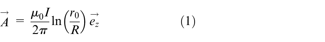
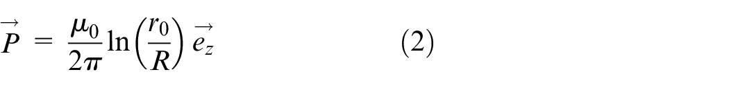
Where
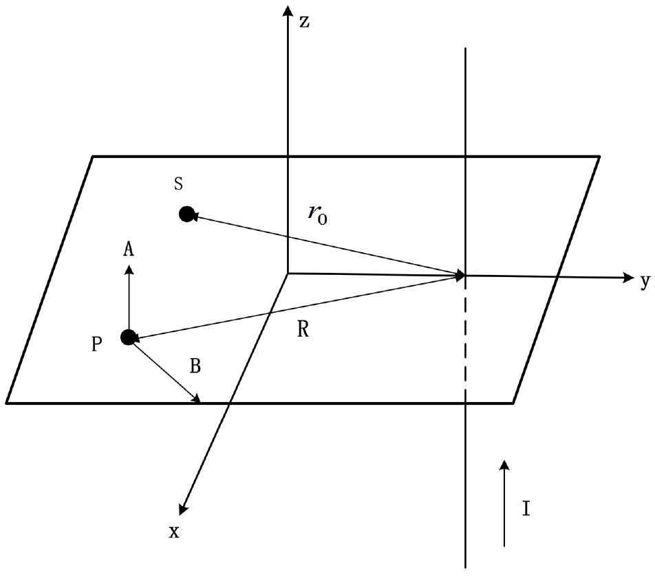
Magnetic potential and magnetic induction intensity created by an infinitely long current.
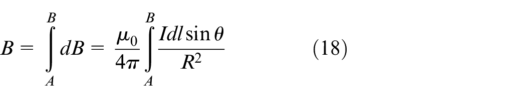
Magnetic induction intensity
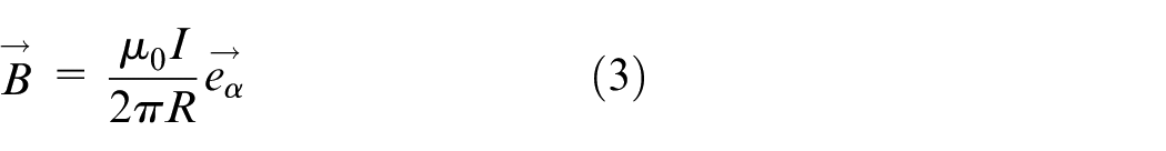
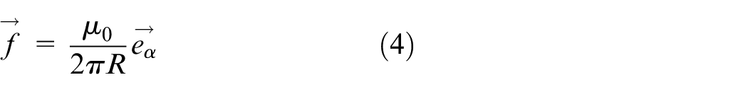
Where
The solution process of SCM is shown in Figure 2. Firstly, the parameters are set, including matching points, check points, the number and position of simulated current. After the parameters are set, equations are constructed to solve the size of simulated current. Then, the magnetic potential error of the check points is calculated by using the obtained simulated current. If the error meets the requirements, use this set of simulated current to calculate the magnetic field distribution; otherwise, reset the parameters and perform the calculation until the magnetic potential error of the check point meets the requirements.
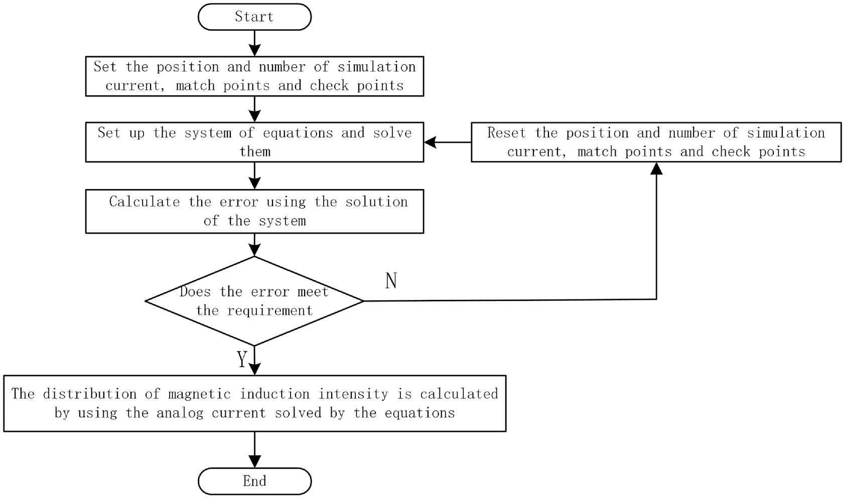
The flow chart of the SCM.
3-D Calculation method
The 2-D model sees transmission lines as infinitely long straight wires, but the reality is that the lines between the towers are under their own gravity. Therefore, the 2-D calculation method cannot accurately calculate the distribution of magnetic induction intensity under the transmission line. So, we need to derive the equations of overhead transmission lines at first. We assumed that the overhead transmission line is a flexible cable chain, and the mass of the overhead transmission line is uniformly distributed to simplify the problem. Based on the assumptions, the wire is catenary in shape.
Figure 3(a) is the overhead line. Point
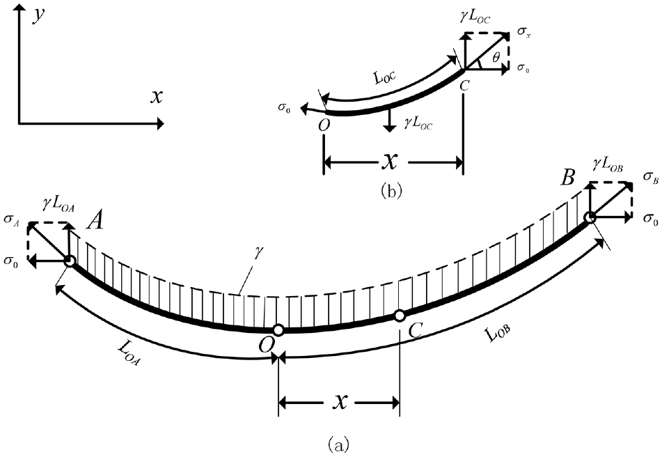
The force analysis diagram of the overhead line: (a) The overhead line, (b) Diagram of force at point C.
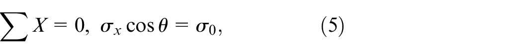
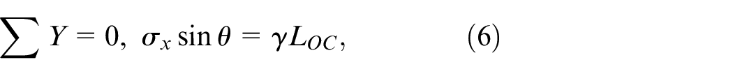
Equation (5) shows that the overhead lines in office point
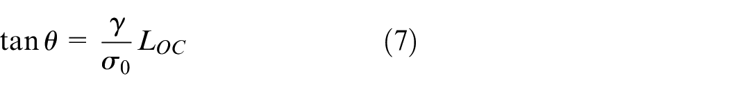
That is:
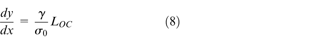
Equation (8) is the differential form of the catenary equation, we can find that when the ratio of
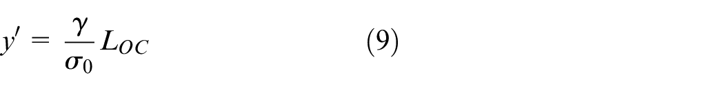
by differentiating both sides of the equal sign of the equation (9), it can be obtained:
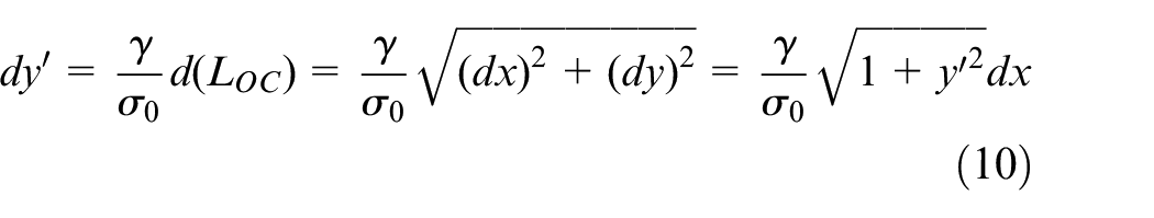
By separating variables and integrating on both sides of the equal sign of equation (10), it can be obtained:
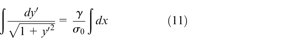
Namely
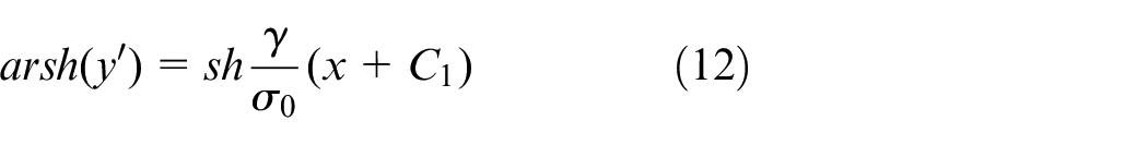
rewrite:
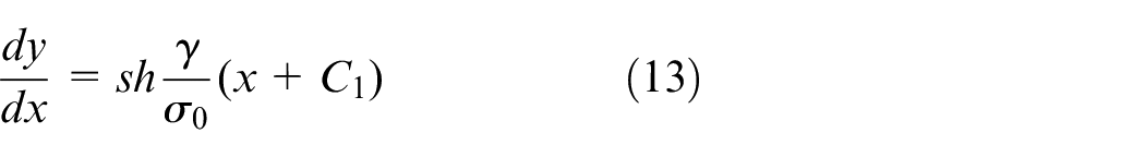
by integrating both ends of formula (13), it can be obtained:
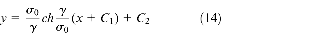
Equation (14) is the general form of integral of the catenary equation. Where
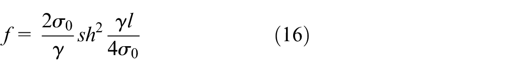
To simplify the calculation, the catenary equation of the same high suspension point is analyzed. Because of symmetry, the lowest point of the overhead line is in the center of the interval. The origin of coordinates is set at this point, as shown in Figure 4.
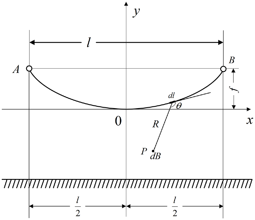
The catenary of the same high suspension point.
When
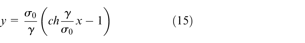
By the formula (15) can be seen, the overhead catenary shape completely by the ratio of
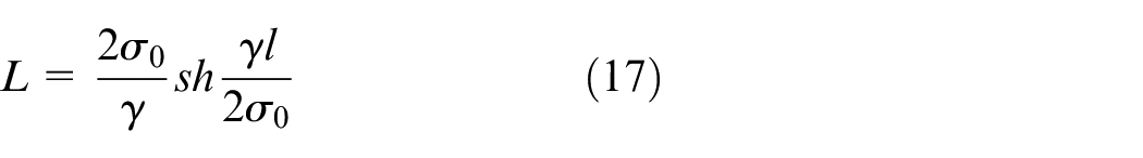
As shown in Figure 4, each current element
Optimize simulation current method
The key of SCM is how to determine the position, number, and shape of simulated current. Once these parameters are determined and the magnetic potential error of the check-points meets the requirements, the equations for solving the simulated current are determined. Therefore, the accuracy of the calculation results will be affected by these parameters. In SCM, the values of these parameters are determined by experience, but the experience is uncertain, so the calculation accuracy is difficult to guarantee and there are many other factors that can influence the actual distribution of magnetic fields, such as trees and metal towers in space, overhead ground wire and the earth’s own magnetic field. Because the error of these factors on the results is small and too random, all the studies conducted in this paper ignore the influence of these factors.
Since the research object is the transmission line, the shape of the simulated current is determined as the line current. In the OSCM, the position and number of simulated currents are determined by the intelligent optimization algorithm, and the flow chart is shown in Figure 5. The SCM was defined as a function of the position and number of the simulated current. First, the parameters of the intelligent optimization algorithm and the independent variables of the SCM function are initialized. Then after calculating the results of magnetic induction intensity distribution, the value of fitness function is calculated. Finally, the independent variable of SCM is updated according to the value of fitness function, until it completes the loop, and the distribution result of magnetic induction intensity is obtained.
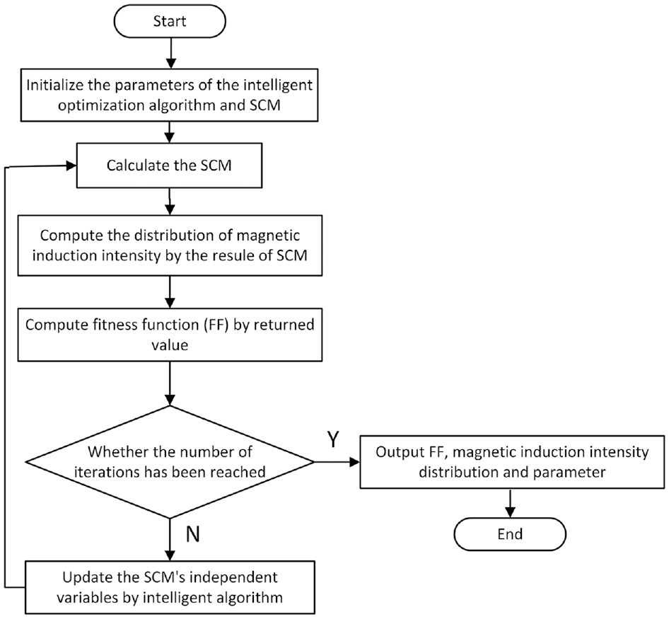
The flow chart of OSCM.
Particle swarm optimization
Particle swarm optimization (PSO) is a global random search algorithm based on swarm intelligence, which simulates the migration and clustering behavior of birds in the process of foraging. PSO was first proposed by Kennedy and Eberhart.
32
The PSO is one of the effective parallel optimization methods, and it was paid more attention to by many researchers in recent years.33–35 In PSO, each potential solution of optimization problem is a bird in the search space, called a particle, all particles have a decided by be optimized function value, the fitness of each particle has a velocity determine their moving direction and location of the particle following the current optimum particles search in the solution space. The updating formulas of velocity
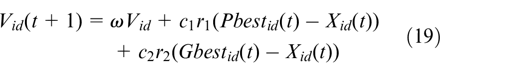

where
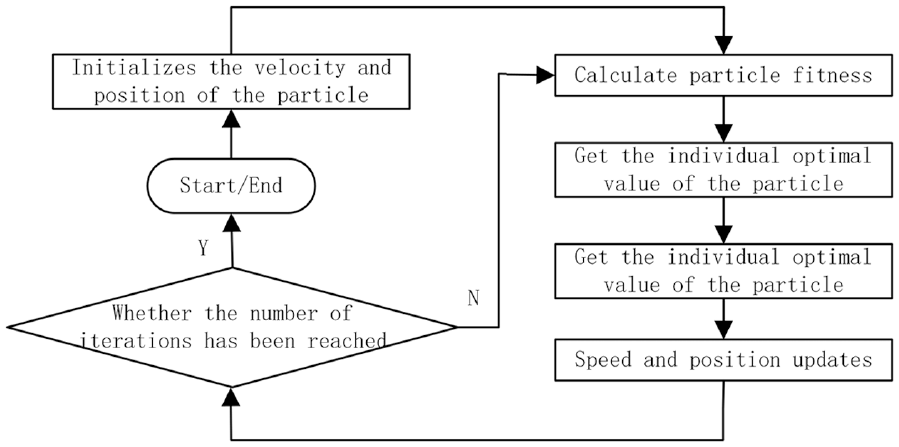
The flow chart of PSO.
Differential evolution algorithm
The differential evolution (DE) algorithm is proposed by Storn and Price. 36 The DE is derived from the genetic algorithm (GA). The core operation of DE includes three parts: variation, crossover, and selection. Different from GA, the variation vector of DE is generated by the difference vector of the parent generation. Therefore, DE is more effective. The flow of DE is shown in Figure 7.
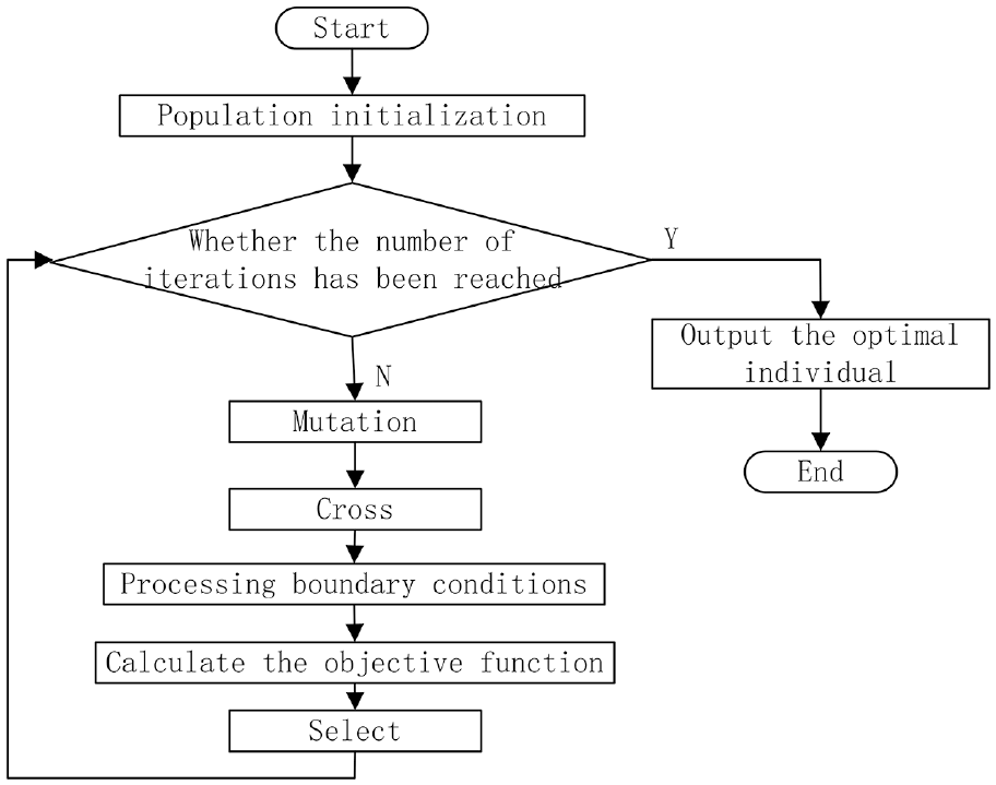
The flow chart of DE.
There are many variation mechanisms of DE, and the most commonly used method is:

where
Commonly used crossover methods include binomial crossover and exponential crossover, in which binomial crossover refers to generating a 0–1 random decimal number for each component. The crossover is performed when the random decimal is less than the crossover operator. The larger the crossover operator coefficient is, the larger the information transmitted by the mutation individual is. On the contrary, the smaller the crossover operator is, the stronger the local search ability is. 37 The cross formula is as follows:
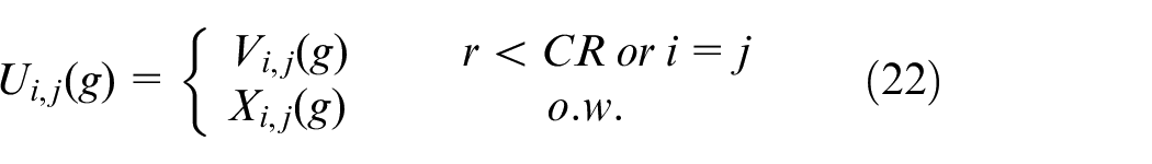
Where
Selection operation in differential evolutionary algorithm refers to comparing the fitness function value of the current population individual and the cross individual to select the good individually as the next generation of the population individual.
Fitness function
In the SCM, the number and position of the simulated current directly affect the calculation result of magnetic induction intensity. In the 3D calculation model, the calculation result is also affected by the shape of the simulated current.
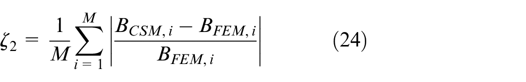
In order to make the calculation result of the SCM more accurate, the fitness function is constructed and the position and number of simulated currents are optimized. The fitness function consists of the mean magnetic position error of the match points and the check points in SCM and the error of magnetic induction intensity calculated by SCM and FEM.
The magnetic potential error between match points and check points
The distribution of match points, check points, and simulated current on the equivalent conductor cross section is shown in Figure 8.
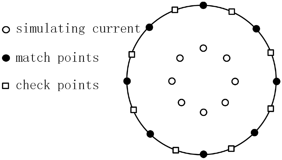
The distribution of match points, check points, and simulated current.
In a high-current system, the skin effect and the proximity effect of the wire are relatively significant, which means that the magnetic induction intensity inside the wire tends to zero. In this case, the surface of the wire can be regarded as an equal magnetic potential line. Therefore, the magnetic potential of the matching point and the check point on the same wire should be equal theoretically. The magnitude of each simulated current and the magnetic potential
Error of SCM and FEM
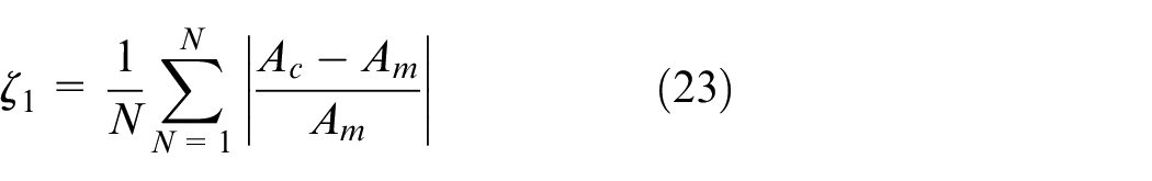
The calculation accuracy of magnetic induction intensity under overhead transmission line by SCM is affected by the number and the position of simulated current. It is also affected by the shape of the simulated current in the 3-D calculation model. In order to obtain these parameters, we used the results of FEM to test the results of SCM. MAXWELL software is used to build the 3D computing model, set the initial conditions and solution domain, and divide the grid adapted. Under the same initial conditions, the average error calculated by the SCM and the FEM is:
Where
Composition of fitness function
The fitness function constructed is the calculation error, and the optimization algorithm is used to find out the location of its minimum value, to obtain the parameters of simulated current, and then the optimal parameters of simulated current are used to solve the magnetic induction intensity. The fitness function is:

The value of
Results and discussion
Analysis of examples
Because of the low current of low-voltage transmission lines, the magnetic field they generate is also very weak, which is easily affected by external conditions and almost harmless to the human body. In the high voltage transmission lines, 1000 and 750 kV transmission lines account for a small proportion. 500 kV transmission line technology is very mature, accounting for more than 95%, 38 and its magnetic field is also large. Therefore, this paper takes the 500 kV transmission line as the calculation model, and the transmission power is 1000 MW, as shown in Figure 9. The lowest suspension point of the transmission line is 24.8 m above the ground, and the conductors of each phase are spaced as shown in the figure. The distance l between the two towers is 400 m. The type of conductor used is LGJ-500/45 four split steel core aluminum stranded wire.
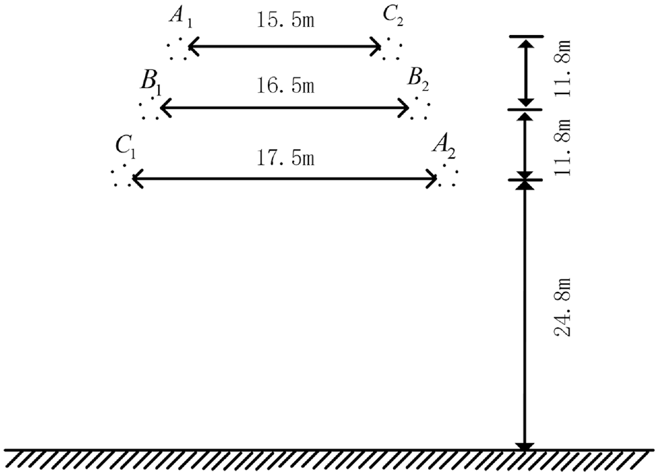
The distribution diagram of three-phase overhead line.
Results of traditional methods
We use the simulation current method and the finite element simulation to solve the above examples, and get the corresponding magnetic field distribution results.
Results of SCM
First, the split wire is simplified as a cylindrical wire, and its equivalent is 8 :
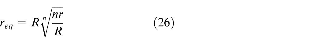
Where req is the equivalent radius,
According to the distribution in Figure 8. With the first matching point as the reference point of zero magnetic potential. The following equations can be constructed based on the calculation method of magnetic potential
Where
Under the condition that the magnetic potential error between the match point and the check point meets the requirements, the magnetic induction intensity coefficient of each simulated current is calculated. And the magnetic induction intensity created by the simulated current can be calculated by using formula (3). The actual magnetic induction intensity value to be calculated is obtained by superimposing the magnetic induction intensities. When the calculated height is 1.5 m, the results of three-dimensional magnetic induction intensity obtained by the SCM is shown in Figure 10.
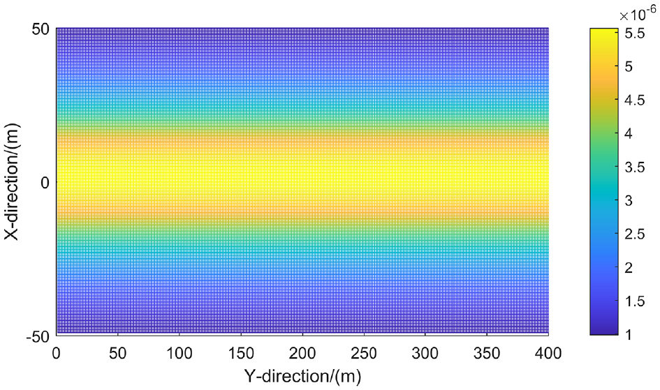
The 3-D calculation results of SCM.
Results of FEM
MAXWELL software was used to simulate and solve the same model. For this practical problem, the simulation conditions are as follows39,40: Maxwell 3D Version 6 is the analysis type; The boundary condition is the default natural boundary condition in software. The excitation condition is current; solution type is magnetostatic; Mesh type and size are adaptive. Maximum number of pass is 10; percent error is 10%; Refinement per Pass is 30%. The calculation results are shown in Figure 11.
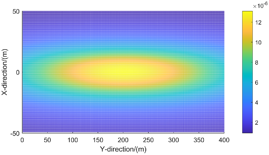
The 3-D calculation results of FEM.
By comparing Figures 10 and 11, it can be find that the two calculation methods have similar results for 3D magnetic induction intensity. The calculation results of the two methods are identical in that the magnetic induction intensity presents unimodal along the X-axis direction. The difference is that the calculation results of FEM show that it presents a convex distribution along the Y-axis, while the results of SCM show that it remains unchanged along the Y-axis. The 2D method regards the transmission line as an infinitely long straight wire, while the 3D method considers the variation of the wire height above the ground. It is not difficult to see from the results that it increases with the decrease of the wire height above the ground.
Figure 12 shows the distribution at different observation points. 2D-SCM is the distribution at height of 1.5 m above the ground obtained by the 2D calculation method. 3D-SCM1 is the distribution at y = 0 m and z = 1.5 m obtained by the 3D calculation method, and 3D-SCM2 is the distribution at y = 200 m and z = 1.5 m obtained by the 3D calculation method. The comparison results show that the shape of the wire has an impact on the magnetic induction strength, especially at the position from −20 to+20 m directly below the wire.
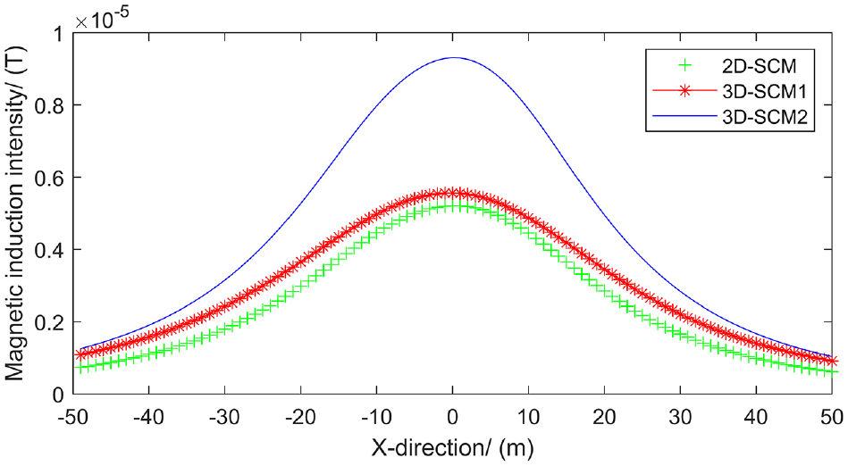
The comparison of magnetic induction intensity.
Optimization SCM and analysis
For SCM, the key is how to select the appropriate number and location of simulated current. Firstly, we use PSO and DE to optimize the position and number of simulated currents. Then combined with the catenary equation of the transmission wire, an OSCM is formed. Finally the magnetic induction intensity is solved.
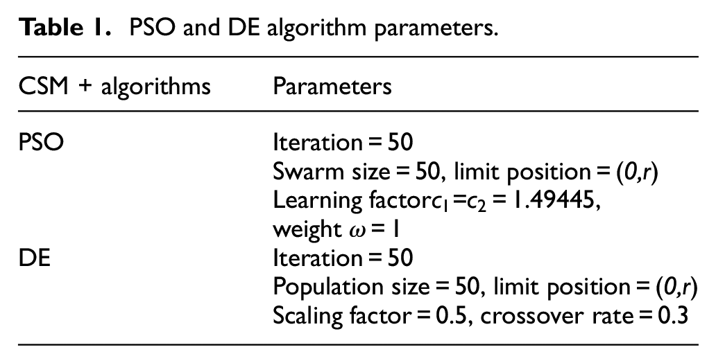
Table 1 shows the calculation parameters of the two intelligent algorithms. To balance the calculation time and convergence of the algorithm, we set the number of iterations and population size of the two algorithms as 50. According to the past experience and experimental results, when the learning factor of PSO is 1.49445 and the inertia weight is 1, the experimental effect is better. The optimization is more efficient when the scale factor and crossover probability of DE are 0.5 and 0.3, respectively.
PSO and DE algorithm parameters.
Parameter optimization based On 2-dimensional model
The positions of simulated current match points and check points are set according to Figure 8. Suppose the search range of the number of simulated currents is 1–15, and the search range of the positions of simulated currents is 0–1 times the equivalent radius.
As shown in Figure 13, with the increase of the number of simulated currents, the magnetic potential error gradually decreases, but at the same time, the computational complexity also increases sharply. As shown in Figure 14, when the simulated current position range is 0.1r–0.4r, the magnetic potential error is small. And the closer the position of the simulated current is to the center, the shorter the mutual distance and the greater the mutual influence. In order to balance the calculation accuracy and calculation error, the number of simulated currents in this paper is 8, and the position coefficient is 0.35.
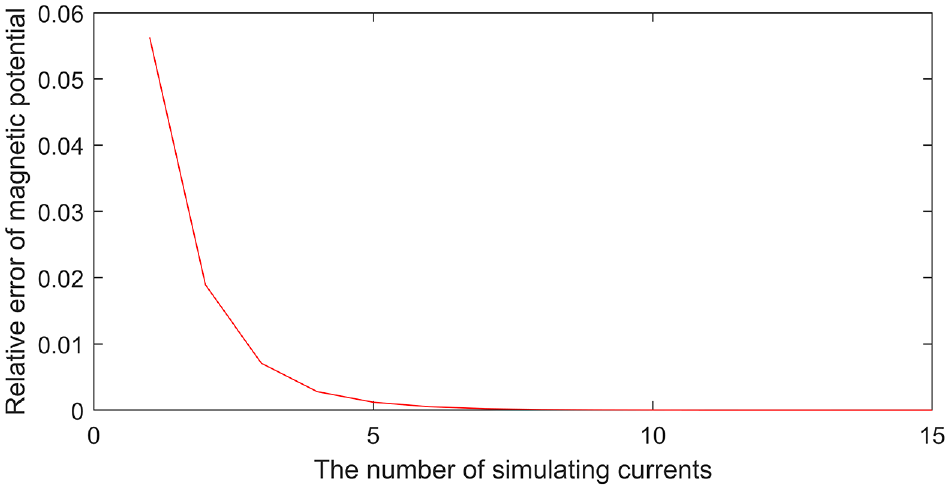
The relationship between the number of simulated currents and magnetic potential errors.
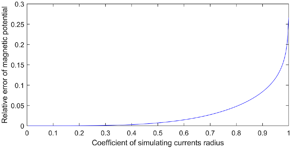
The relationship between position of simulated current and magnetic potential error.
Parameter optimization based on 3-D calculation model
Due to the actual transmission conductor for catenary shape, and the magnetic induction intensity with wire increase with the decrease of the height from the ground. So, consideration of transmission wires as infinitely long and straight leads to a large calculation error. Therefore, after optimizing the position and number of the simulated current, the influence of the actual shape of the transmission wire on the calculation results should be considered. In the example shown in Figure 9, the optimization algorithm is combined with SCM, and the actual shape of the transmission line is taken into account to calculate 3D magnetic induction intensity. After 50 iterations, the convergence results of the two optimization algorithms are consistent.
In Figure 15, PSO and DE are respectively used to optimize the fitness function constructed by the equation (25) with a minimum value. The convergence results of the two optimization methods are consistent. After the optimal point is found, the location of the optimal point is recorded, and the number and location coefficient of the simulated current at this time is calculated as 4 and 0.040056, respectively.
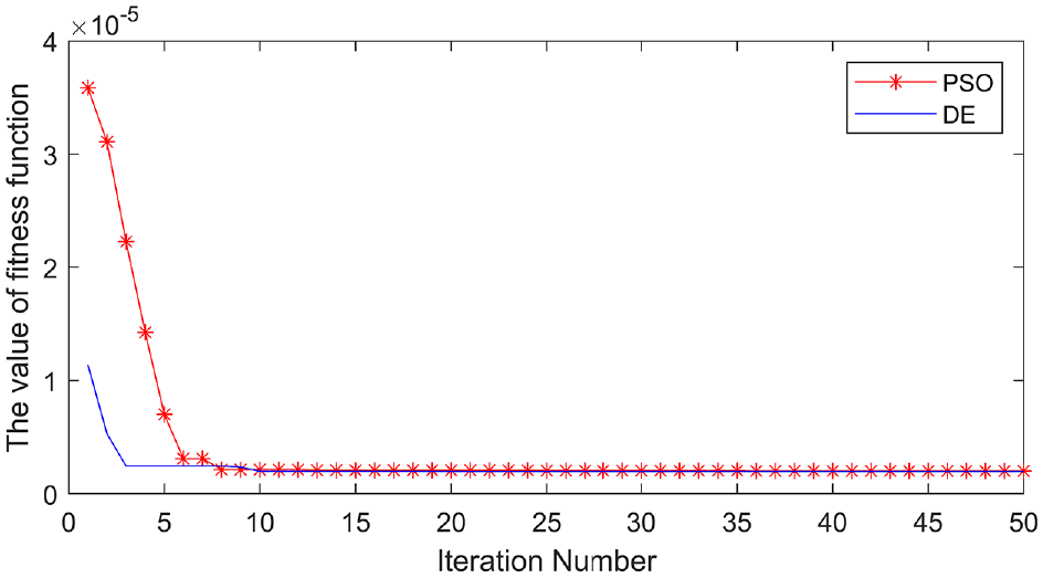
The relationship between the number of iterations and the fitness function value.
Comparison and analysis
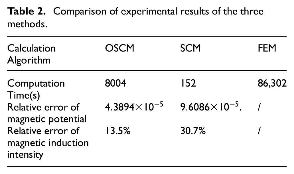
We can find that from Table 2, the calculation time of FEM is as high as 86,302 s due to complex modeling and high calculation accuracy. Due to the added optimization process for PSO/DE, OSCM’s computation time was about 50 times that of SCM, but the computation time was still in the acceptable range. The magnetic potential error of the matching point and the checking point in OSCM is smaller than that of SCM, but the magnetic potential error is within the range of 10−5. In this paper, by using PSO/DE to find the optimal parameters of SCM, and then calculating the magnetic field distribution strategy, the magnetic induction intensity error of OSCM is 13.5% which is significantly lower than 30.7% of SCM. Therefore, combined with calculation time and calculation error, OSCM has a great improvement over the general simulated current method.
Comparison of experimental results of the three methods.
On the observation plane 1.5 m above the ground, the results obtained by three calculation methods are shown in Figure 16. SCM does not consider the sag of the circuit and does not optimize the parameters of simulated current. In order to see the difference between the three results clearly, the results at y = 200 m, z = 1.5 m, and x = [−50,50] were extracted, as shown in Figure 17. The results show that the calculation results are basically the same, but the results of SCM are different from those of FEM.
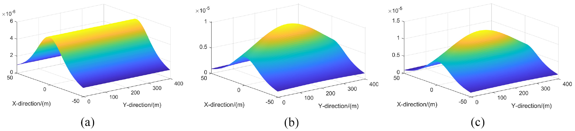
The magnetic induction intensity distributions of SCM, OSCM, and FEM: (a) SCM, (b) OSCM, and (c)FEM.
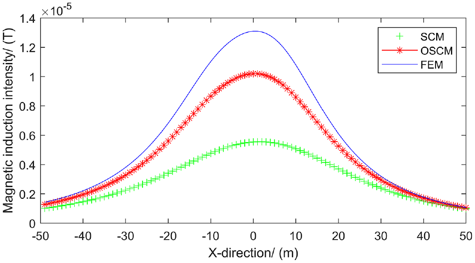
The magnetic induction intensity distribution of SCM, OSCM and FEM (y = 200 m, z = 1.5 m).
The area with high magnetic induction intensity under the line is concentrated in x = [−20, 20]. The value of other regions is very small due to the sharp decrease of magnetic induction intensity, so the significance of the study is not significant. In the region x = [−20, 20], the value of magnetic induction intensity is large and fluctuates greatly. In the region x = [−20, 20], because PSO/DE is used to optimize the parameters, the error of OSCM on magnetic induction intensity is 21.81%, which is 34.9% higher than the 56.71% of SCM.
Conclusions
We calculate the magnetic field distribution under the actual overhead wire using a 3D magnetic induction intensity calculation method based on OSCM. The PSO/DE algorithm was combined with SCM to obtain the optimal simulated current number and its position, and then the magnetic field distribution was solved. The result of PSO is consistent with that of DE, which verifies that the optimization result is not accidental. At the same time, MAXWELL software was used to simulate the same problem, and the results of FEM were used to verify the results of OSCM.
Based on the calculation model of 500 kV overhead transmission line, we use PSO and DE respectively to optimize the SCM. The fitness function of the optimization algorithm is composed of magnetic potential error and magnetic induction intensity error, so that the results are both accurate and robust. The magnetic induction intensity distribution of the OSCM is close to that of the FEM, which indicates that the optimization of SCM by particle swarm optimization and differential evolution algorithm is feasible.
According to the calculation results, the relative error of magnetic potential is
There are still many problems that can be further studied in this paper. In parameter optimization of SCM, the number of simulation current is more conveniently represented by a parameter, while the location parameter is represented by 0–1 times of the equivalent radius. Although this can achieve better optimization, it will set the simulation current in the same circle, which has limitations. Subsequently, multiple parameters can be used to characterize the position parameters of the analog current, so that the simulation current can be distributed in any position within the equivalent radius, there is no limit, so that better position parameters can be found, and the calculation can be more accurate; The influence of different transmission lines on ground height, transmission loop, split conductor and conductor arrangement on magnetic field distribution under the line can also be explored.
Footnotes
Acknowledgements
The authors would like to thank the State Grid Sichuan Electric Power Company maintenance Company. We got the money, the data and the equipment through their project “a wireless power extraction device near an UHV transmission line.”
Author contributions
The authors’ individual contributions are provided as follows: Conceptualization, W.O. and J.Z.; methodology, W.O. and J.Z.; software, W.O. and W.D.; validation, J.H. and W.L.; writing-original draft preparation, W.O. and J.Z.; writing review and editing, W.O., J.H., W.L., and D.W.; supervision, J.Z. and J.H. All authors have read and agreed to the published version of the manuscript.
Declaration of conflicting interests
The author(s) declared no potential conflicts of interest with respect to the research, authorship, and/or publication of this article.
Funding
The author(s) disclosed receipt of the following financial support for the research, authorship, and/or publication of this article: This research was funded by National Natural Science Foundation of China grant number 61705127 and National Natural Science Foundation of China grant number 61902237.