
Abstract
Stabilizing the purchase cost of metal raw materials is of great significance to the metal manufacturing industry. Most enterprises use futures hedging strategies to cope with the risks arising from fluctuations in the prices of metal raw materials. However, the difference between spot and futures prices of metals makes it impossible to fully control the risk. In order to further improve the efficiency of hedging and controlling corporate risks, it is necessary to accurately predict futures prices. However, the decomposition algorithms in traditional mixed models are prone to modal aliasing and have limited ability to extract nonlinear features from futures prices. Therefore, this paper proposes a variational modal decomposition-sample entropy-Cascaded Long Short-Term Memory Neural Network Model (VMD-SE-CLSTM). This paper proposes SE combined with VMD algorithm to determine the decomposition number to suppress the aliasing phenomenon of subsequence patterns, and introduces CLSTM network to improve the extraction ability of nonlinear features in futures data. The experiments are compared with 10 mainstream model methods and the method proposed in this paper. The experimental results show that the model reduces the prediction error and improves the prediction accuracy of the model, which is of great significance for enterprises to improve hedging efficiency, reduce operating risks and control production costs.
Keywords
Introduction
Metal is vital for industrial production. 1 With the rapid development of the modern industry, the enterprises’ demand for metal materials is gradually rising, denoting that metal materials have an important role in social development. 2
Changes in metal futures prices are influenced by a variety of factors, such as monetary policy, environmental protection policy, resource endowment, supply, demand, etc. It is a typical non-stationary time series.3,4 For metal processing enterprises, the purchase cost of raw materials can account for more than 60% of enterprise costs, 5 and price fluctuations can have a significant impact on enterprise production. Hence, enterprises wish to establish a profit and loss hedging mechanism between the metal raw material futures market and the spot market through hedging strategies to reduce the risks associated with futures price fluctuations.6,7 Among them, hedging strategy refers to a company’s trading in the spot market and futures market in equal but opposite directions, expecting to buy or sell futures at some point in time to compensate for the price risk caused by price fluctuations in the spot market. The error between spot and futures is called the forward margin. 8 The premise of this strategy is that the volatility of the forward margin is highly coordinated. However, the volatility of the forward margin is obvious, and when the difference is too large, it is difficult to hedge risks using conventional financial means. Therefore, if we can achieve accurate forecasting of metal futures prices in the futures market, we can guide enterprises to improve the effectiveness of hedging, which helps them to achieve overall cost control in production and operation and avoid the risk of metal raw material price fluctuations. 9
With the continuous development of the futures market, two types of futures price forecasting models have been formed: traditional single forecasting models and hybrid forecasting models. 10 A traditional single forecasting model is one in which data are simply processed and fed directly into the model for forecasting. Dooley and Lenihan compared the results of a lagged futures price model and an autoregressive integrated moving average model (ARIMA) for forecasting lead and zinc price series and found that ARIMA achieved better forecasting results. 11 Although statistical models have improved forecasting performance to some extent, they all have inherent limitations and have a smaller range of applications. Statistical models can capture the linearity of the data, however, there are many non-linearities in the price series of metal raw materials. As a result, statistical models cannot achieve good prediction accuracy. 12 In recent years, the use of artificial intelligence models for time series forecasting has become more and more widely used. 13 Liu et al. used decision trees to predict the short- and long-term changes in copper prices and achieved robust prediction results with better prediction accuracy than traditional regression models, 14 but traditional artificial intelligence models dealing with time series tend to fall into local optima. 15 Among them, the recurrent neural network-based improved long- and short-term memory network (LSTM) has obvious advantages in time series modeling, improving the long-term dependency problem in Recurrent Neural Networks (RNN), and is suitable for modeling time series. 16 Compared with other time series prediction models, LSTM has a more complete network structure with the design of forget and memory gates and has better prediction ability for highly nonlinear time series data, which can improve the long-term dependency performance of the model.17,18 Muzaffar and Afshari used LSTM networks to predict short-term electric load changes and achieved better prediction accuracy than statistical models and traditional neural networks. 19 However, Futures price series data are highly complex and the traditional single model has many limitations in forecasting.20,21
Accordingly, a hybrid model was developed. The basic idea is to address the shortcomings of a single model and generate a synergetic effect in forecasting. 22 Hybrid models are generally divided into two types: time-series hybrid prediction methods based on residuals and time-series hybrid prediction methods based on decomposition-aggregation.23–25 Among them, the hybrid model based on the decomposition-aggregation principle decomposes the time series data into multiple subseries, reducing the volatility of the series and capturing the trend of the series more easily. 26 The model can effectively improve the forecasting accuracy and is suitable for futures price series forecasting. Empirical mode decomposition (EMD) is an adaptive signal decomposition algorithm proposed by Huang. 27 It decomposes sequence data into smaller frequency components, which can be referred to as intrinsic modal components (IMFs). The decomposed IMF has lower volatility, which is convenient for model analysis and processing. EMD uses a recursive approach to decompose the data. Decomposition usually over-decomposes the series, which leads to the gradual accumulation of decomposition errors. Especially when there are jump changes in the data, the decomposition is likely to produce modal confounding, and the series values will fluctuate up and down several times and with large amplitude in a very short period of time, affecting the accuracy of prediction. 28 Xian et al. combined ensemble EMD and independent component analysis to predict the price of gold, extract deep features in the sequence, and obtain better prediction results. 29 Complete Ensemble Empirical Mode Decomposition with Adaptive Noise (CEEMDAN) 30 added a limited adaptive white noise to EEMD 31 to solve the incompleteness and reconstruction error of EEMD with the addition of white noise. Lin et al. used a hybrid model combining LSTM and CEEMDAN to forecast stock price changes, comparing a single model with a hybrid model, and achieved the best prediction effect. 32 Both EEMD and CEEMDAN algorithms solve the modal aliasing phenomenon by adding white noise to the original sequence. None of the above decomposition algorithms can separate components with similar frequencies, which limits the decomposition effect of the sequence. 33 Decomposition methods such as EEMD will decompose the sequence too much, and residual white noise will cause information interference. The non-original data added in the decomposition method changes the original information of the data and affects the accuracy of prediction. 34
We propose a VMD-SE-CLSTM network futures price forecasting hybrid method, which can be applied to hedging strategies, which can effectively enhance the ability of metal processing companies to respond to fluctuations in raw material prices and reduce the risks caused by market price fluctuations. VMD has a solid theoretical foundation and can decompose a time series into sub-sequences of a specific bandwidth and a specified number. 35 We use the SE algorithm 36 to calculate the SE of the sub-sequence and determine the decomposition number K to prevent the original sequence from being over-decomposed, which obviously suppresses the modal aliasing phenomenon, and does not change the original data.37,38 The SE algorithm is usually used to characterize the irregularity and complexity of the signal, and to quantify the regularity and unpredictability of the time series. Compared with approximate entropy, 39 the calculation of SE does not depend on the length of the data, has better consistency, and is suitable for measuring the complexity of financial time series. At the same time, to better extract the nonlinear features in the futures sequence data, we introduced the cascaded long-term short-term memory network, which has more nonlinear structures and deeper network levels and can better extract the features in the sequence data. 40 Enterprises can predict the changing trend of the closing price of the futures market through the proposed model and implement the hedging trading strategy in the futures market, thereby reducing the risks caused by market price fluctuations and weakening the risks caused by raw material market price fluctuations.
This study has the following contributions:
In order to better suppress the modal aliasing phenomenon in the decomposition process, we propose SE combined with the VM algorithm to clarify the decomposition number K in the variational modal decomposition process, measure the complexity of the subsequence, and prevent the original sequence from being overly decomposed.
To better extract nonlinear features in futures sequence data, we introduce a cascaded long short-term memory network. Based on this, a decomposed hybrid model VMD-SE-CLSTM combined with the futures market hedging strategy is proposed to reduce the risk of market price fluctuations.
By comparing with the single model, the advantages of the mixed model in futures price forecasting are proved. At the same time, the proposed hybrid model is compared with 10 mainstream models, and the best prediction accuracy is obtained.
This paper is arranged as follows: Section 2 introduces the framework of the hybrid model and algorithms in the models. Section 3 presents the futures data and evaluation index and model parameters in the study. Model comparison experiments and back-testing experiments are presented in section 4. Section 5 summarizes the full text.
Methods
Model construction for metal futures hedging
Considering the non-stationarity, autocorrelation, and asymmetry of the spot price series and futures price series. In this paper, we introduce the GJR (1,1) model 41 with negative information correction term to fit the expected volatility and expected volatility of the time series of asset returns. The GJR (1,1) model is constructed as:


On day
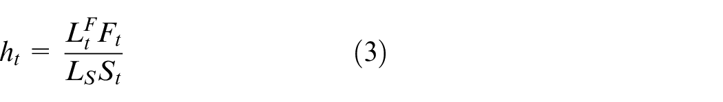
In the portfolio, the amount of spot planned to be hedged is constant, and the hedge ratio is a variable that changes dynamically over time. Therefore, the expected return rate
This paper reduces the risk of market price fluctuations by predicting the price changes of raw material futures. The hedging strategy is the most commonly used risk hedging scheme in the futures market. Therefore, the GJR model is introduced here for illustration. The core parameter in the GJR model is rt, the predicted value of the asset return at time t, which can be obtained from the mixed model in Section 2.2. Therefore, the predictive effect of the model is directly related to the effect of the hedging strategy. Decision makers can execute corresponding trading strategies by predicting price changes.
The proposed hybrid method
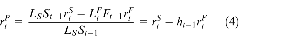
This study aims to propose a hybrid method for futures price prediction, while identifying the appropriate decomposition number, performing VMD decomposition to decrease volatility, and extracting features via the CLSTM model. The model frame structure is exhibited in Figure 1. Initially, the original futures data are imported and the original data and other preprocessing operations are normalized to integrate the data into the decomposition algorithm. After which we use the VMD decomposition algorithm to decompose the original sequence, calculate the SE of the subsequence, and select the most appropriate number of decomposition K. Decompose the original sequence into K subsequences and input them into the CLSTM network. Thereafter, the appropriate decomposition number k is determined according to SE and the sub-sequence data are incorporated into the CLSTM network. Finally, by synthesizing the prediction results of each sub-sequence, the final prediction result is obtained.
Flowchart of the VMD-CLSTM method.
VMD
VMD is a completely non-recursive mode decomposition and signal processing method proposed by Dragomiretskiy and Zosso. 35 Its decomposition process involves the construction and elucidation of variational problems. Notably, a relatively stable sub-sequence with multiple frequency scales can be decomposed by iteratively searching for the optimal solution of the variational model so that the center frequency and bandwidth of each decomposed component can be determined. VMD can decompose data into specific frequency sub-sequences, such that the bandwidth of each sub-signal in the frequency domain has a specific sparse nature. Thus, the VMD decomposition algorithm can be applied to the volatile futures price data to reduce the complexity of the sequence, suppress the appearance of modal aliasing, and obtain more sequence features.
VMD is used to decompose the original input signal
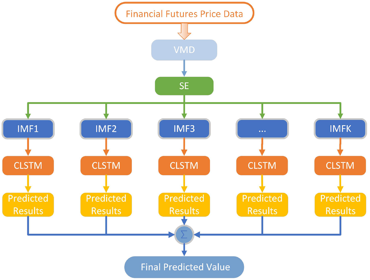
The VMD construction constrained variational problem is as follows:
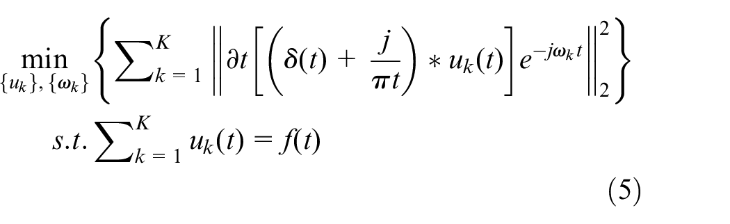
where
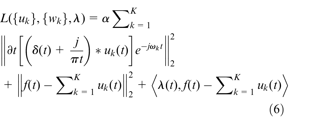
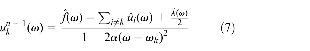
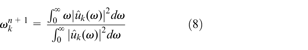
Using the alternating direction method of multipliers, the saddle point of the augmented Lagrange expression is updated iteratively, and optimal solutions are obtained. The iterative update method is as follows:
SE
SE is used to measure the complexity of time-series signals based on the approximate entropy method. It uses a nonnegative number to represent the complexity of time series and reflects the richness of information contained within. Compared to approximate entropy, SE has two advantages: the calculation of SE does not rely on the length of the data; the change of parameters
(1) For a time-series consisting of N data
(2) Reconstruct a set of vector sequences of dimension m,
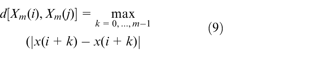
(3) We define the distance
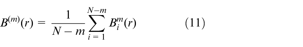
(4) For a given
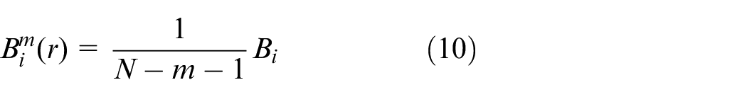
(5) Define
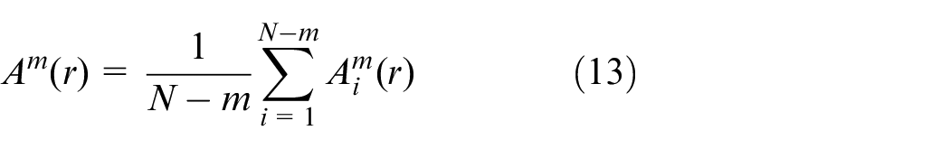
(6) By increasing the dimension to
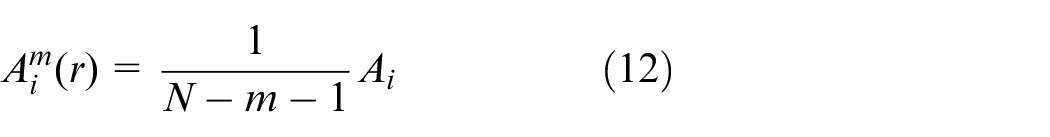
(7)

When N is a finite value, it can be estimated using the following formula:

CLSTM
LSTM is an improved recurrent neural network derived from RNN, which is used to solve the problem of gradient disappearance or explosion caused by training long-distance dependent data. Hence, it is suitable for time series, natural language processing, and other fields. The LSTM network mainly controls the input door and the forgotten door in the network structure to determine the information remembered and forgotten about the network. Moreover, the output door is also regulated to determine the output value.
The difference between the CLSTM network emphasized in this study and the traditional LSTM network is that the former can extract the main features of the time series to better fit the trend of futures prices. Primarily, the cascading structure of the model can increase the depth of the network and further extract the main features of the sequence. Moreover, adding nonlinear units can enhance the characteristics of time series, and the improved gating mechanism can better memorize the characteristics of the input sequence. The network structure diagram of CLSTM constitutes the following three parts (Figure 2):
Part I:
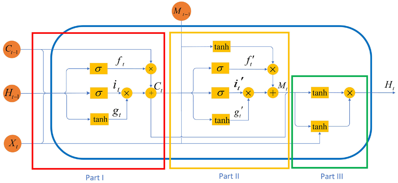
Schematic diagram of the CLSTM network structure.
The first part is to adjust on the basis of LSTM; the difference is that the current state


where
Lastly, the forgetting gate is multiplied by the last time state, and the input gate is multiplied by the control gate to acquire the updated unit state

Part II:
The network structure of the second part is similar, but the nonlinear operation is completed before the
The process of the second part is similar to that of the first part. The gate is determined by the input


where
Finally, a nonlinear operation is performed on

Part III:


The
Experimental data and index design
In this section, we introduce the datasets used in this study, the statistical metrics of the experimental results, and the setting of relevant parameters in the algorithm. These futures returns were traded from January 2010 to December 2019, lasting for approximately 10 years. The futures transaction data of each trading day are considered as the raw data, including opening price, highest price, lowest price, closing price, trading volume, and so on.
Dataset
The futures data used in this study come from four raw material futures markets in Shanghai (i.e. RB, AL, CU, ZN), comprising futures contracts with the longest trading time and the largest trading volume in the Shanghai futures market. RB represents the raw material of rebar, AL aluminum, CU copper, and ZN zinc. The data are obtained from https://www.joinquant.com/data (accessed on June 24, 2021), which can be downloaded in the sub-category of “Futures Data” under the grouping of “Data Dictionary.” The data can also be downloaded for free through github (accessed on June 24, 2021). After downloading the original data, it is normalized and then divided for each of the futures. The first 65% of the data were employed as the training set, 15% were used as the validation set, and the last 20% were utilized as the test set. Consequently, the training, validation, and test datasets of four futures with labeled data can be obtained.
Evaluation criteria
The loss error is usually used to evaluate the prediction effect and better evaluate the prediction ability of the model. Notably, this research uses three evaluation indexes. The smaller the value of the evaluation index, the better the prediction effect, including the root mean squared error (RMSE), mean absolute error (MAE), and mean absolute percentage error (MAPE). Meanwhile, the goodness of fit (
Metrics used for the evaluation of regression effects.
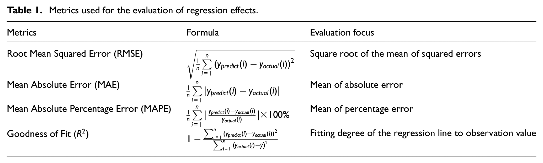
In Table 1,
MAE is the average value of the absolute error and reflects the error of the predicted value, which can better reflect the actual situation of the predicted value error and is a more general form of the average value of the error. MAPE is expressed as a percentage and has nothing to do with the ratio but can be used to compare the forecasts of different ratios. The smaller the three indicators of RMSE, MAE, and MAPE, the lower the prediction error of the model and the better the prediction effect.
Parameter settings
Model parameter settings
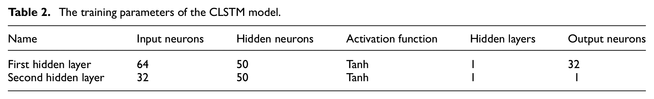
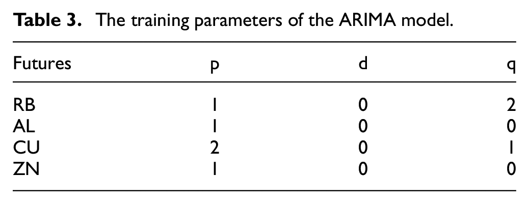
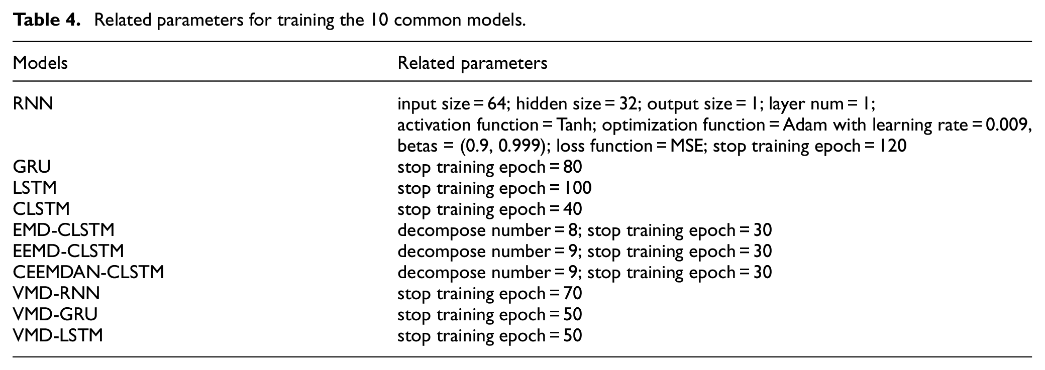
Here, we explain the setting of the CLSTM network model parameters, as demonstrated in Table 2. The model parameter table is shown in Tables 3 and 4.
The training parameters of the CLSTM model.
The training parameters of the ARIMA model.
Related parameters for training the 10 common models.
In the SE algorithm, the SE value is related to the values of
The parameter selection in the above parameter table is found through grid search, and the fairness of the comparison between models is ensured by selecting the optimal parameters in the model. Epoch is the number of training iterations for which the model is most suitable by early stopping.
Determination of the decomposition number K
This study uses a variational model to decompose the input futures price series. Among them, the key parameter decomposition number K had a greater impact on VMD decomposition. If the chosen decomposition number K happens to be too small, the sequence data will not be fully decomposed, and the volatility of the sub-sequence will still be large. Conversely, if the decomposition number is too large, the sequence data will be over-decomposed, but the difference in the sub-sequences will be small, the decomposition accuracy shall be reduced, and the modal aliasing phenomenon will also occur.
This research employs SE to measure the complexity of a sequence signal. The larger the SE, the higher the complexity of the sequence. According to the change in SE of the sub-sequence, it is determined whether the sequence is fully decomposed to ascertain the appropriate decomposition number K.
The change trend of SE after the decomposition of different futures price series are displayed in Table 1. Interestingly, the trend changes first increase and then decrease. When the value of K selected by VMD decomposition is small, the original futures price sequence is not fully decomposed. After the sequence is decomposed, the value of the SE increases instead. When an appropriate decomposition number K is selected, the SE is at a turning point, implying that the complexity of the sequence is reduced after decomposition. Still, the sequence will be over-decomposed when we choose a very large decomposition number K, and modal aliasing shall occur easily.
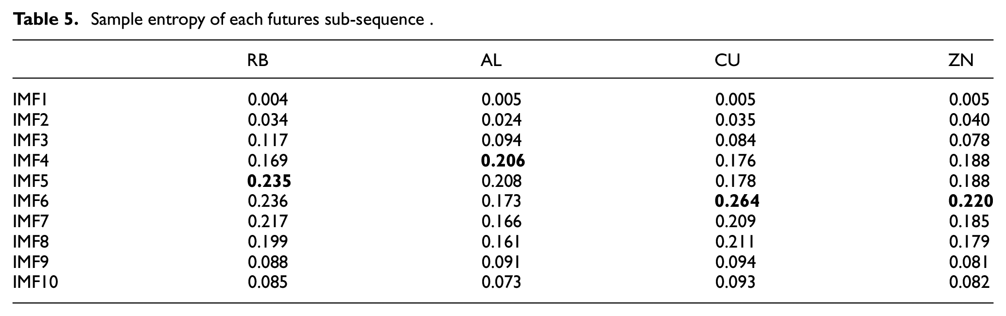
According to decomposition Table 5 of the rebar price sequence, when the number of sub-sequences is less decomposed, the intricacy of the sequence is lower, and the phenomenon of sub-sequence spectrum aliasing can be effectively suppressed, but the SE value gradually increases. When K is 5, the SE value reaches its maximum threshold, and the entropy value of the subsequent decomposition sample decreases, indicating that when K = 5, the sequence is fully decomposed. We choose the K value at the turning point where the SE tends to be smooth to prevent excessive decomposition of the original price series. The black bold part in the table is the K value of the selected decomposition number of the futures price selected by the model. Thus, 5 is chosen as the decomposition number for the rebar futures price series. Likewise, we can obtain the decomposition number of AL futures price as 4, the decomposition number of CU futures price as 6, and the decomposition number of ZN futures price as 6.
Sample entropy of each futures sub-sequence .
Experiments
In this section, the SE algorithm is used to determine the complexity of the sub-sequence and choose the appropriate decomposition number for the futures price. Then, we compare the prediction results of the single model and the mixed model with regard to the futures data. EMD, EEMD, CEEMDAN, and VMD are employed to decompose the futures price sequence and then compare the forecasts. We then compare the methods to determine the effect of the VMD decomposition number K on the model prediction effect. Additionally, we use the VMD decomposition method and the same decomposition number for the model predictions, and compare the results to the conventional regression algorithm to visualize the prediction effect of our model.
Comparison of mixed model and single model
Figure 3 highlights a comparison of evaluation indicators concerning five types of neural network models for different futures (i.e. RB, AL, CU, ZN) price series predictions.
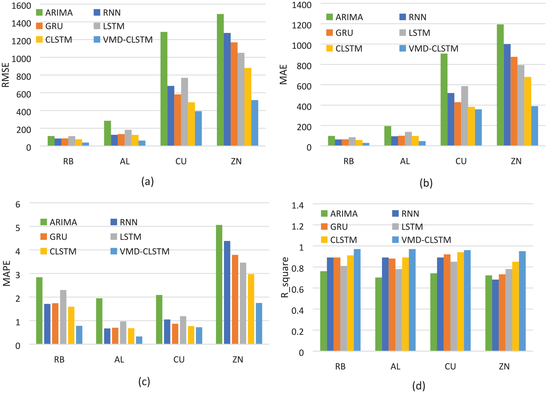
(a) Sequence diagram of the comparison of RMSE between mixed model and single model, (b) sequence diagram of the comparison of MAE between mixed model and single model, (c) sequence diagram of the comparison of MAPE between mixed model and single model, and (d) sequence diagram of the comparison of
Compared with the traditional statistical model ARIMA, the neural network model has higher prediction accuracy for financial futures time series. For example, it can be seen from the RMSE, MAPE, and MAE in Figure 3 that the prediction error of the mixed model VMD-CLSTM is less than that of a single model. Furthermore, the mixed model has the highest degree of fit for futures prices from the perspective of the goodness of fit. Compared to the single-model prediction method, the hybrid model combined with the decomposition algorithm has a good prediction effect, improves the prediction performance of the model, and minimizes the prediction error. Moreover, in the comparison between prediction and evaluation indicators of a single model, the prediction effect of the CLSTM network was better than that of the conventional time series model. When we adjusted the number of hidden layers of the model for experimental comparison, we found that increasing the depth of the model failed to improve its accuracy.
Evaluating the effectiveness of the VMD algorithm
Different decomposition algorithms are used to decompose the original sequence, including EMD, EEMD, CEEMDAN, and VMD. Subsequently, the CLSTM network is utilized to predict the sub-sequence. The outcomes obtained for the different futures price forecasts are depicted in Figure 4.
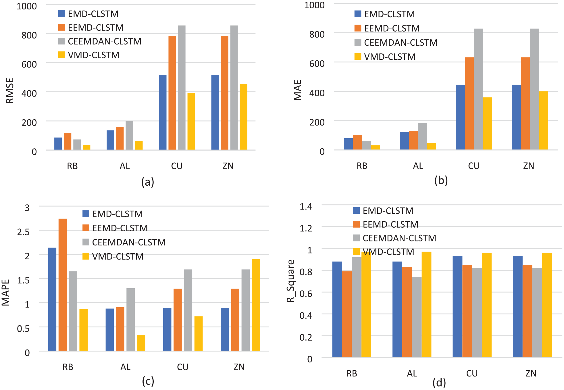
(a) sequence diagram of the comparison of RMSE of futures data forecasts with different decomposition methods, (b) sequence diagram of the comparison of MAE of futures data forecasts with different decomposition methods, (c) sequence diagram of the comparison of MAPE of futures data forecasts with different decomposition methods, and (d) sequence diagram of the comparison of
VMD has better prediction accuracy than different futures price series decomposition methods based on EMD, EEMD, and CEEMDAN (refer to Figure 4), signifying that VMD has a better futures price sequence decomposition effect. Algorithms such as EMD adopt the self-use decomposition method, which leads to excessive decomposition of the sequence and reduction of the prediction accuracy of the model. The evaluation indexes RMSE, MAPE, and MAE obtained from the VMD decomposition prediction in the experiment were also lower, and the prediction results were more accurate. This finding confirms that using the VMD decomposition method to decompose the original data can provide more sequence information and reveal the characteristics of each component more completely. The sub-sequence obtained through VMD decomposition is more stable, so the prediction of the sub-sequence after decomposition can provide a prediction result with a smaller error and better fitting degree.
Evaluate the validity of sample entropy to determine K value
In this study, we used the SE algorithm to determine the K value of the VMD decomposition algorithm. The EMD method is typically used for the data first, and the K value determined by the EMD method is used as the K value of the VMD algorithm. 33
The experiment compares the VMD decomposition number K determined by two different decomposition methods and proves that using SE to find the decomposition number can improve the prediction ability of the model. The futures price sequence is decomposed by VMD using different decomposition numbers. Thereafter, the decomposed sub-sequences are incorporated into the CLSTM network for prediction, and the final result is obtained. The results of predicting a variety of futures prices are listed in Table 6.
Influence of different decomposition numbers of VMD on the prediction.
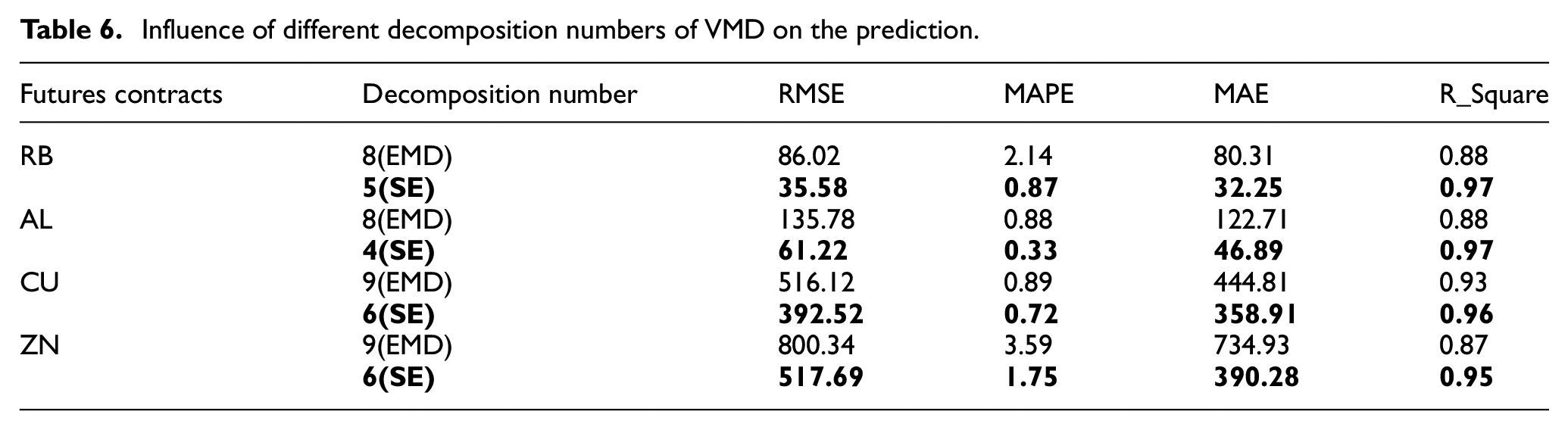
The SE algorithm selects the appropriate decomposition number by judging the change trend of the entropy value. It can be seen from the table that the decomposition number K determined by SE can achieve better prediction accuracy and smaller prediction errors than the general K value determination method. From the goodness of fit index, the decomposition number determined by SE also has a better decomposition effect on the original data.
Evaluation of the proposed hybrid model
VMD is employed to decompose the original price series and use different networks for predictions. The proposed VMD-CLSTM model can obtain more accurate prediction results, outlining that a combination of VMD and CLSTM networks can better capture the nonlinear and deep features of the original sequence (refer to Table 7). For the four raw material futures datasets, the prediction effect of the proposed VMD-CLSTM prediction model is the most accurate, validating that the proposed model has good prediction accuracy and robustness for various types of futures.
Influence of different decomposition numbers of VMD on the prediction.
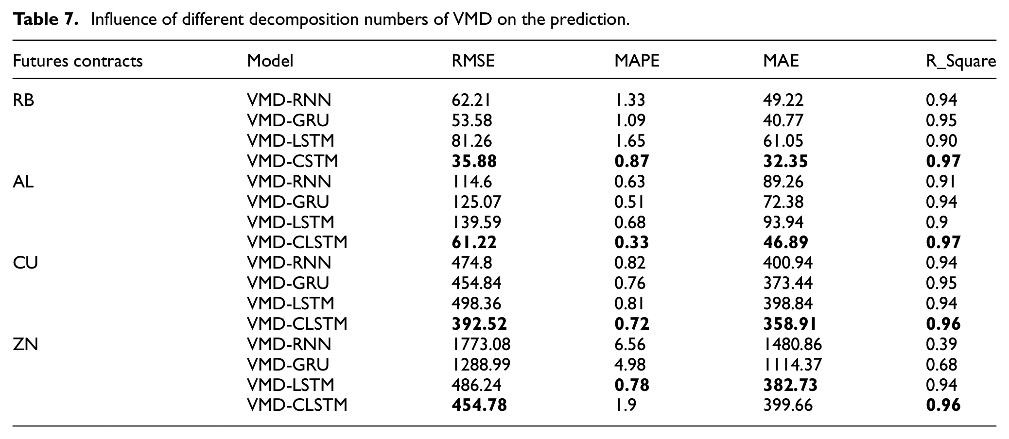
The VMD-CLSTM model shows good performance in raw material futures price forecasting and achieves the best accuracy in the above-mentioned comparison model. The MAPE, RMSE, and R side of VMD-CLSTM in the rebar futures sequence prediction were 0.87, 35.58, and 0.97, respectively. Meanwhile, the mixed model threaded steel futures forecast error is the smallest (refer to Figure 6(a)). Compared with other benchmark models, the MAPE and RMSE of VMD-CLSTM are smaller, relaying that the prediction effect of the model is better than that of the benchmark model, with a better effect in futures price prediction. From Figure 5(a), we can see that the rebar futures price prediction curve can better fit the price trend and has the highest goodness of fit. We use VMD-CLSTM to predict on other futures prices and obtain better forecast accuracy and smaller forecast errors, as shown in Figures 5 and 6. Compared with other models, this model has smaller prediction errors for out-of-sample futures prices, indicating that the model is more robust.
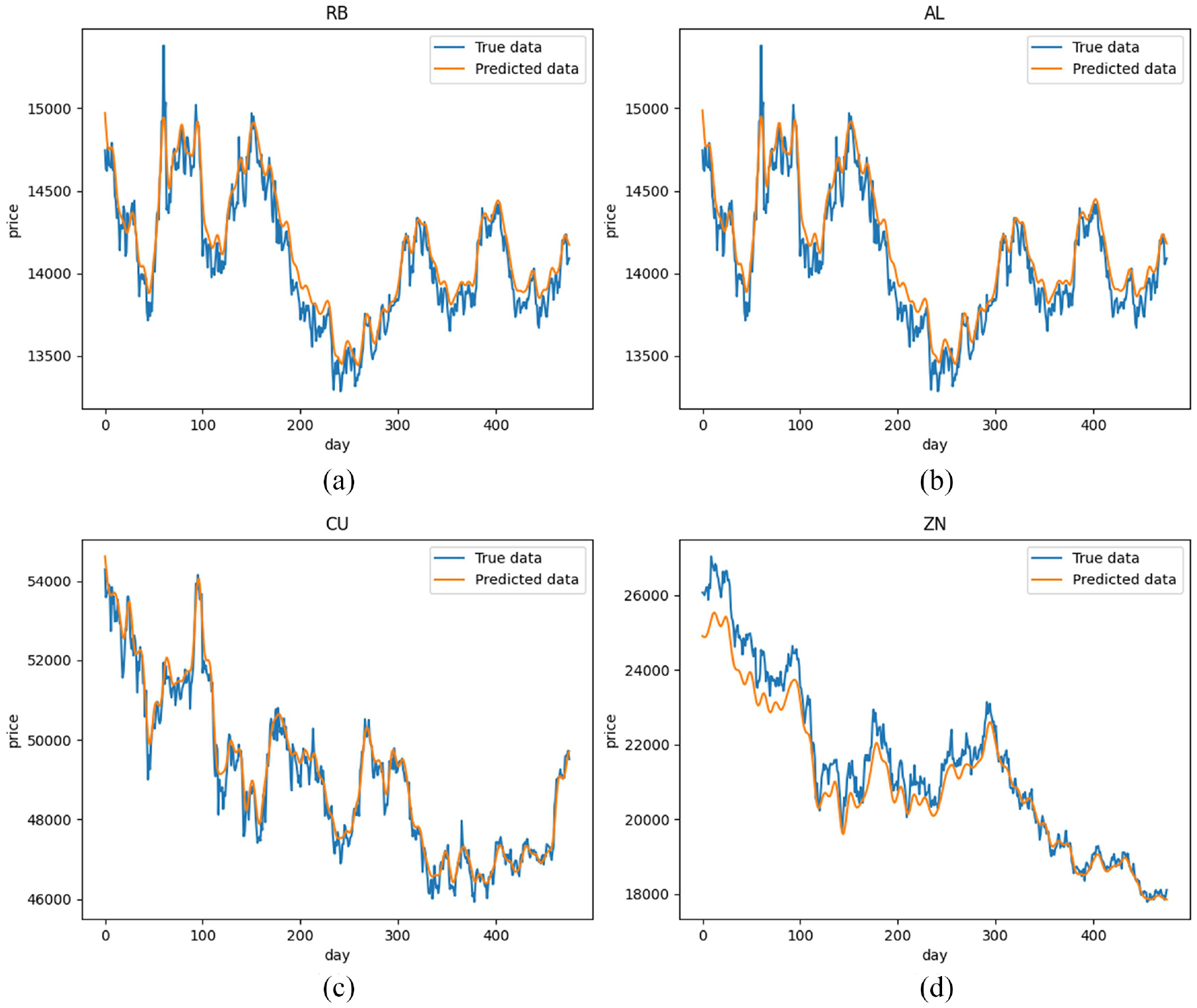
(a) VMD-CLSTM rebar futures price prediction results, (b) VMD-CLSTM aluminum futures price prediction results, (c) VMD-CLSTM copper futures price prediction results, and (d) VMD-CLSTM zinc futures price prediction results.
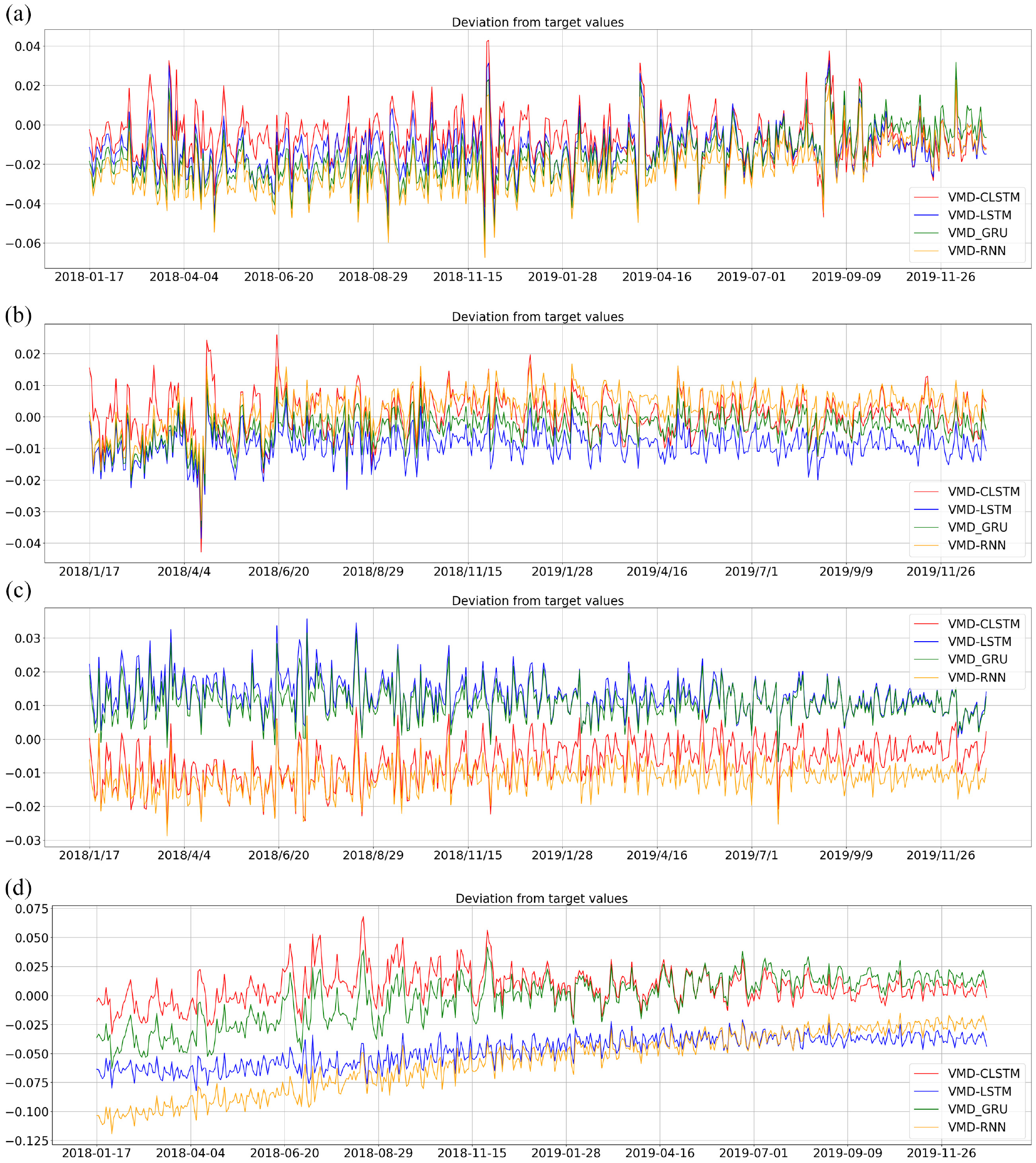
(a) Four hybrid models predicting deviation from target values of rebar futures, (b) four hybrid models predicting deviation from target values of aluminum futures, (c) four hybrid models predicting deviation from target values of copper futures, and (d)four hybrid models predicting deviation from target values of zinc futures.
As can be seen from Figure 5(d), due to the impact of the global epidemic from 2019 to 2020, the unilateral market situation of zinc futures has led to persistent deviations in all models, and the statistical characteristics of the market have been weakened. A good forecast is achieved, but overall, the model can make the best forecast for most futures prices
Evaluation of simulated trading
Using four mixed models of LSTM, GRU, RNN, and CLSTM transactions are carried out according to the predicted change trend of rebar futures prices. In this simple trading strategy, we buy the futures if the next day’s opening price is predicted to be above the current day’s opening price, accounting for the transaction costs.
As illustrated in Figure 7, the test data time range was 476 days in total (i.e. approximately 2 years). The average return rate of the VMD-RNN model is 33.21%, the average rate of return of the VMD-GRU model is 50.62%, the average rate of return of the VMD-LSTM model is 62.43%, the average rate of return of the VMD-CLSTM model is 103.26%, and the results show that under the same initial capital premise, the four futures simulated by the VMD-CLSTM model have the highest average yield, followed by VMD-GRU, VMD-LSTM, and finally VMD-RNN.
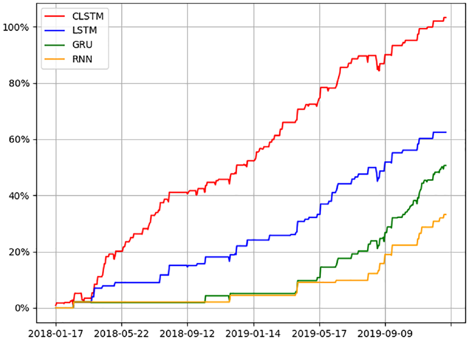
Four hybrid models simulating the futures price of rebar.
Figure 7 shows excess returns that can be obtained by all prediction models. Higher excess returns can be achieved because VMD-CLSTM has a better prediction effect. For enterprises, futures can be purchased or sold through a hedging strategy to reduce the risk in the current market.
Conclusions
This paper proposes a hybrid model, VMD-CLSTM, to predict changes in daily raw material metal prices. First, we decompose the original data based on the VMD decomposition algorithm, and decompose the original data fully according to the decomposition number K value determined by the SE value. Afterward, the decomposed sub-sequence is trained by the CLSTM network. The four data sets of the Shanghai Futures Exchange were then evaluated using three error indicators (RMSE, MAPE, and MAE) and the goodness of fit (
Research Data
sj-csv-1-mac-10.1177_00202940221105868 – Supplemental material for Risk control of metal raw materials based on deep learning
Supplemental material, sj-csv-1-mac-10.1177_00202940221105868 for Risk control of metal raw materials based on deep learning by Chen Zhao, Yexin Wang, Yuefeng Cen, Lebin Wu and Jie Zhou in Measurement and Control
Research Data
sj-csv-2-mac-10.1177_00202940221105868 – Supplemental material for Risk control of metal raw materials based on deep learning
Supplemental material, sj-csv-2-mac-10.1177_00202940221105868 for Risk control of metal raw materials based on deep learning by Chen Zhao, Yexin Wang, Yuefeng Cen, Lebin Wu and Jie Zhou in Measurement and Control
Research Data
sj-csv-3-mac-10.1177_00202940221105868 – Supplemental material for Risk control of metal raw materials based on deep learning
Supplemental material, sj-csv-3-mac-10.1177_00202940221105868 for Risk control of metal raw materials based on deep learning by Chen Zhao, Yexin Wang, Yuefeng Cen, Lebin Wu and Jie Zhou in Measurement and Control
Research Data
sj-csv-4-mac-10.1177_00202940221105868 – Supplemental material for Risk control of metal raw materials based on deep learning
Supplemental material, sj-csv-4-mac-10.1177_00202940221105868 for Risk control of metal raw materials based on deep learning by Chen Zhao, Yexin Wang, Yuefeng Cen, Lebin Wu and Jie Zhou in Measurement and Control
Footnotes
Author contributions
C.Z.: Resources, supervision, conceptualization, methodology and project administration. Y.W.: Programing, validation of the results, analyses, writing & editing, and data curation. Y.C.: Resources, supervision and project administration. All authors have read and agreed to the published version of the manuscript.
Declaration of conflicting interests
The author(s) declared no potential conflicts of interest with respect to the research, authorship, and/or publication of this article.
Funding
The author(s) disclosed receipt of the following financial support for the research, authorship, and/or publication of this article: This work was supported by the National Natural Science Foundation of China under Grant 61902349.
Data availability statement
The data are from https://www.joinquant.com/data (accessed on 24 June 2021), under the “Futures Data” sub-category of the “Data Dictionary” category. The data are also available for free through ![]() (accessed on 24 June 2021).
(accessed on 24 June 2021).
References
Supplementary Material
Please find the following supplemental material available below.
For Open Access articles published under a Creative Commons License, all supplemental material carries the same license as the article it is associated with.
For non-Open Access articles published, all supplemental material carries a non-exclusive license, and permission requests for re-use of supplemental material or any part of supplemental material shall be sent directly to the copyright owner as specified in the copyright notice associated with the article.