
Abstract
In this paper, several methods about the active noise control (ANC) system are studied. The common adaptive recognition system based on the variable step filter x least mean square (FxLMS) algorithm are elaborated. By introducing the momentum term into the variable step algorithm, the value range of the variable step is increased, so as to speed up the convergence of the algorithm and improve the effect of noise reduction. The weight of the control filter based on the improved logarithmic function variable step size least mean square (VSSLMS) algorithm is updated in the improved second channel online recognition algorithm. The initial smooth noise signal, the noise signal of increasing amplitude, and the abrupt noise signal are utilized to verify the convergence speed and the noise reduction effect of the modified ANC method. Numerical results show that the improved algorithm structure could improve the convergence speed and reduce the noises of the whole system at three different primary noises. The initial smooth noise signal, the noise signal of increasing amplitude, and the abrupt noise signal are utilized to verify the convergence speed and the noise reduction effect of the modified ANC method. Numerical results under three different primary noises show that the improved algorithm structure could improve the convergence speed and reduce the noise of the whole system.
Introduction
Noise is ubiquitous and affects our daily lives. A high-noised environment for a long time will seriously affect people’s physical and mental health. The noise originates from the various household appliances, such as the air conditioning, washing machines, refrigerators, cutting machines, ventilation ducts, compressors, and generators. Thus, noise control is essential.
Generally, passive noise control and active noise control are two effective methods to suppress the noise.1,2 Traditional noise control methods use passive noise control (PNC) techniques such as sealing and shielding to attenuate noise. However, such methods suffer from the bulky volume, expensive cost, and degradation performance for reducing low-frequency noise, which hinders its practical use. 1 Active noise control (ANC) is one of the most effective methods to control noise. 3 However, the LMS algorithm used by the traditional ANC system has a contradiction in terms of convergence speed and steady-state error, that is, to make the algorithm converge quickly, the result of steady-state error is very large, so the LMS algorithm must make a compromise.4–6 With the upgrading of hardware equipment, the calculation speed of the optional ANC controller is faster and faster, and the complexity of the computable algorithm is also higher and higher, which provides the possibility for the application of the more complex variable step size LMS algorithm in practice.7–9 The LMS algorithm is improved by the algorithm proposed in Refs.10–20 to solve this spear shield. Large stride length is applied to these algorithms so that the system converges quickly in the initial step. When the system gradually converges, the step-size factors begin to reduce, and the system maintains a small steady-state error. These algorithms are expressed by various step factors. The sigmoidal function is used to control the step length factor, and the algorithm in Davari and Hassanpour 15 and Zhang and Zhang 17 is improved based on Akhtar et al. 14 Besides, the arctangent function 16 and hyperbolic tangent function are used to control step-length factors19,20 are used to control the step-size factor, respectively.
Although the above algorithms have been greatly improved in terms of convergence speed and steady-state error performance, complex calculation, slow convergence, and poor tracking performance still occur in the above algorithm.10–20 Therefore, a new variable step size LMS algorithm based on logarithm function is proposed in this paper, and the improved algorithm is applied to ANC system of online modeling of secondary channels.
Variable step-size LMS algorithm
The traditional ANC system uses LMS algorithm to update the weights. 8 Its basic structure is shown in Figure 1.
Basic block diagram of LMS algorithm.
The LMS algorithm is a random implementation of the steepest descent algorithm. Cost function


where
In the N-tap transverse filter, the transient behavior of the steepest descent algorithm depends on the sum of N exponents. Each exponent is controlled by eigenvector R of the autocorrelation matrix. Eigenvalue


Variable step-size LMS algorithm based on the logarithmic function
Compared with “exponential,”“sine,” and other methods, the logarithm function is relatively simple without much calculation. Moreover, if the step factor and the error signal can form a logarithmic relationship, both the convergence rate and steady-state error will be improved. Key factors

where a controls the overall change of the curve; m controls the change speed at the bottom of the curve; b is the magnitude of the curve. The influence of the values of a, b, and m on the step-size curve is also discussed. Too large “a” value causes the step-size factor to miss the optimal value. These parameters should be selected reasonably in the practical application 21
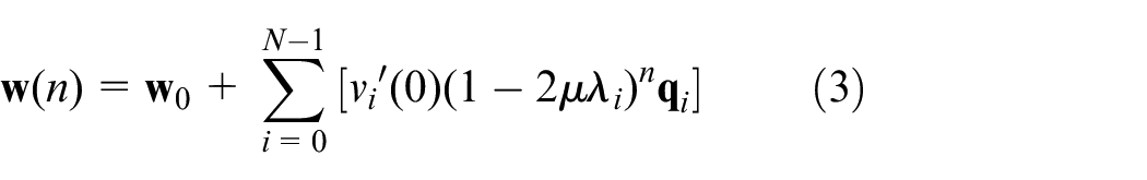
MLMS algorithm
The MLMS algorithm is improved based on the LMS algorithm. 22 A momentum term is added in the process of weight-coefficient adjustment. The algorithm is described as follows. 23
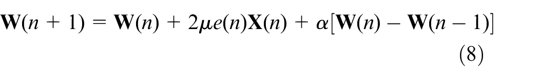
where
The correlation of weight coefficients is used in the adaptive adjustment process, and momentum term
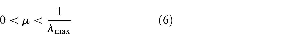
The convergence condition of the MLMS algorithm
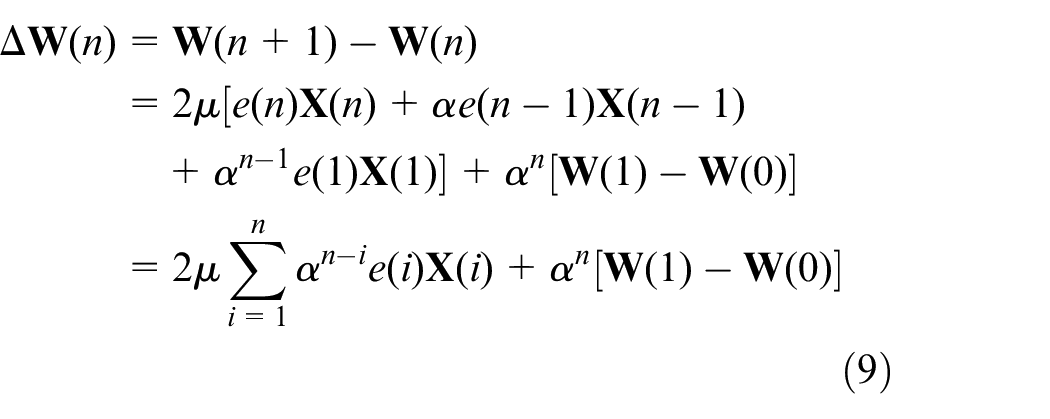
Equation (9) converges under the following conditions:

For the specific derivation process of the convergence range of the step-size factor, please refer to Tan et al. 22 and Gao and Xie. 23 The expression of the critical convergence coefficient of the system is as follows.
It is almost the same as the critical value expression of the convergence step factor of the LMS algorithm in form, except that the constant factor of MLMS is multiplied by another
Modified method
The basic step-size adjustment principle of the variable step-size adaptive filtering algorithm is to keep a large step size factor in the initial stage to converge the algorithm. When the error signal is relatively stable, the step-size factor is adjusted to a small value, 14 which reduces the steady-state error. The reference error is greatly less than 1 in the steady-state stage. The increased orders of the error term improve the steady-state performance in the step-size variation algorithm. The modified variable step-size LMS adaptive filtering algorithm is extended as:
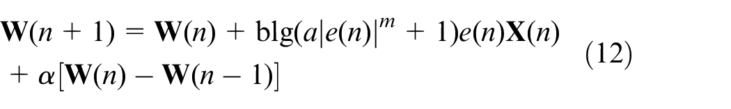
where step factors a, b, m and momentum factor
This algorithm is based on the variable step-size LMS algorithm in Zhou.
21
By adding constant 1 to logarithm function
Figure 2 describes the comparison of error values with/without the momentum term, the smooth noise signals with a variance of 0.1 is used as a primary noise signal. The red line represents the added momentum term (
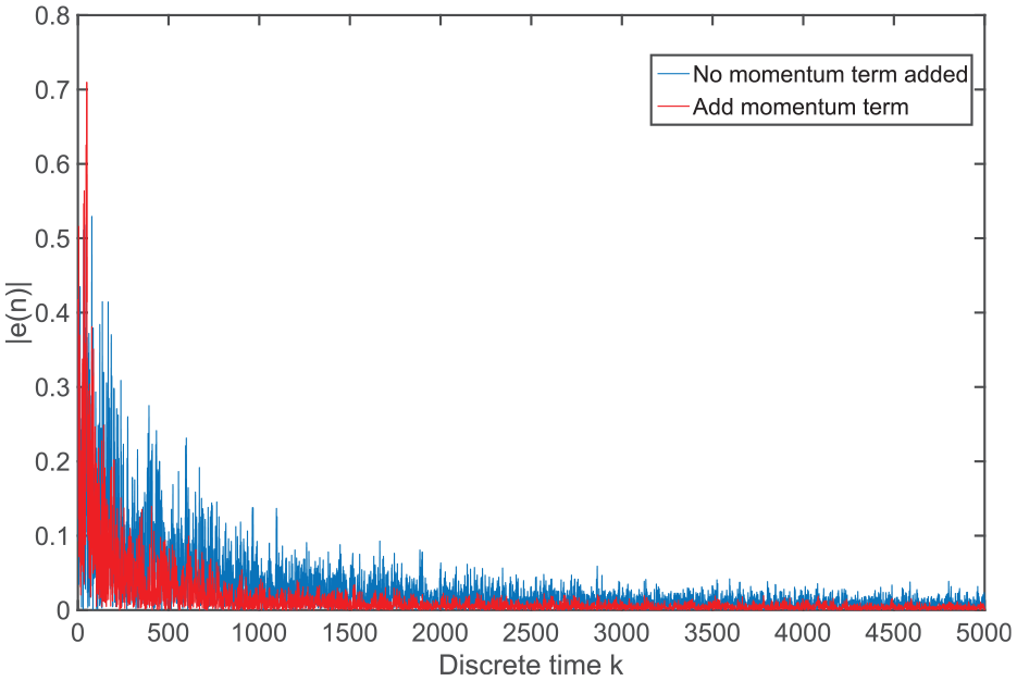
Comparison of error values with/without the momentum term.
The measurement standard is defined as the follows to intuitively compare the improved the algorithm by different momentum coefficients.25–27
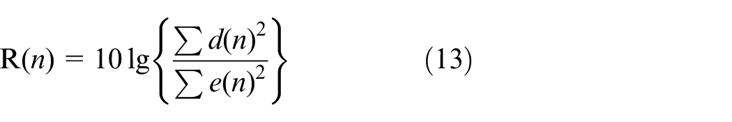
where
Figure 3 illustrates the convergence curve at different values. The noise reduction effect gradually improves with the increased momentum term at
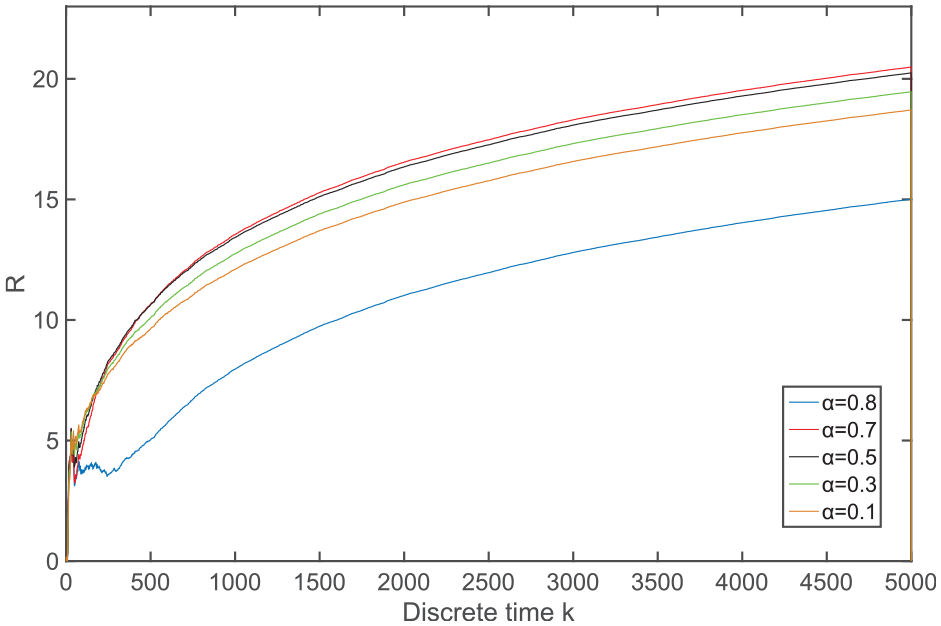
Convergence curves corresponding to different
When
In Figure 4, when the discrete-time is higher than the step of 1000, the noise reduction of the improved algorithm is higher than that of the previous method. Besides, the noise-reduction gradient gradually increases with time, demonstrating the noise reduction effect of the improved logarithmic function term.
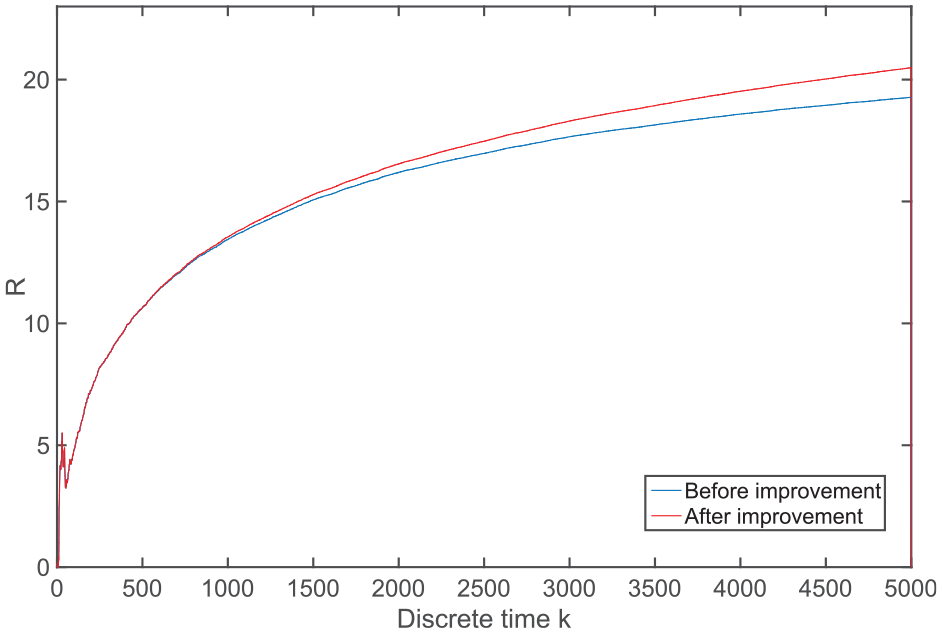
R-value comparison between the previous method and the improved logarithmic function term.
Online modeling approach for secondary channels
Several existing online modeling methods for ANC secondary channels are described in the following section, and the improved algorithm is introduced to optimize the convergence rate and steady-state error.
In the actual physical system, the secondary signals processed by the LMS algorithm need to be output through the secondary loudspeaker before being offset with the primary noise. The error signals are fed back to the ANC controller after the acoustic-sensor acquisition, filtering, and A/D conversion. Secondary-channel S(z) is included in the DAC unit, smoothing filter, power amplifier, speaker, acoustic channel from the speaker to error sensor, error sensor, preamplifier, anti-aliasing filter, and ADC unit.
Effective secondary-channel estimation is essential. The convergence step size consistently changes, and the iterative steps constantly increase. The system cannot be stable when the improper estimation makes the difference between the phase estimate of the transfer function and the actual value greater than 90°. In general, both offline and online modes are included in secondary-channel estimations.
Predecessors method
Figure 5 shows the online modeling system of the secondary path proposed by Eriksson and Allie. 24 Figures 6 and 7 respectively show the improvement schemes of Zhang and Akhtar for the online modeling of Eriksson’s secondary channels. Their work mainly focuses on optimizing the accuracy of the modeling of the secondary channels and maintaining the correctness of the feedback values of the control filter to optimize the original model, and good optimization results have been achieved.
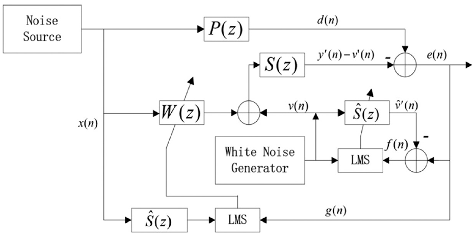
Eriksson’s secondary-path online modeling system.
Zhang’s secondary-path online modeling system.
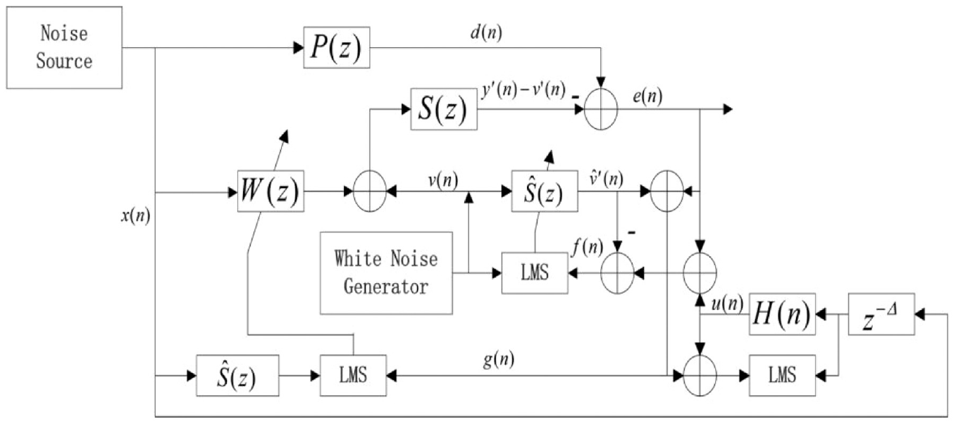
Akhtar’s secondary-path online modeling system.
Propose method
With the upgrading of hardware equipment, the calculation speed of the optional ANC controller is faster and faster, and the complexity of the computable algorithm is also higher and higher, which provides the possibility for the application of the more complex variable step size LMS algorithm in practice.
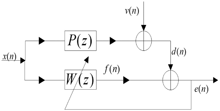
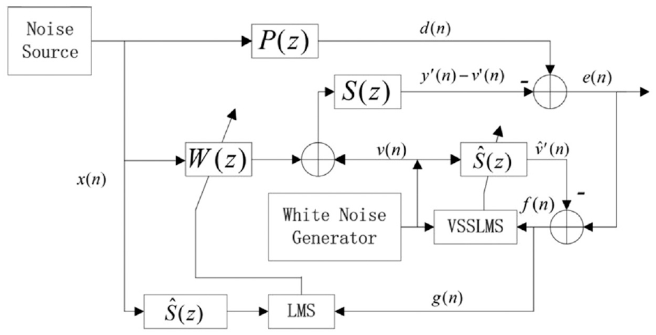
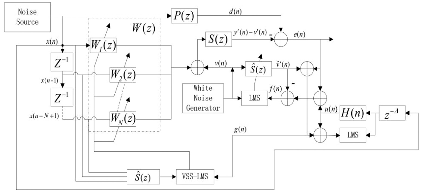
In order to optimize the convergence rate and noise reduction effect, VSSLMS algorithm is considered to optimize and improve Zhang’s model and Akhtar model. Previous optimization schemes focus on the secondary-channel modeling. In this paper, the overall noise reduction effect and convergence rate of the optimization model are considered, so the improved focus is focused on the control filter
The improvement of the above two methods is shown in Figures 8 and 9. VSS-LMS algorithm is used to update the weight of the control filter
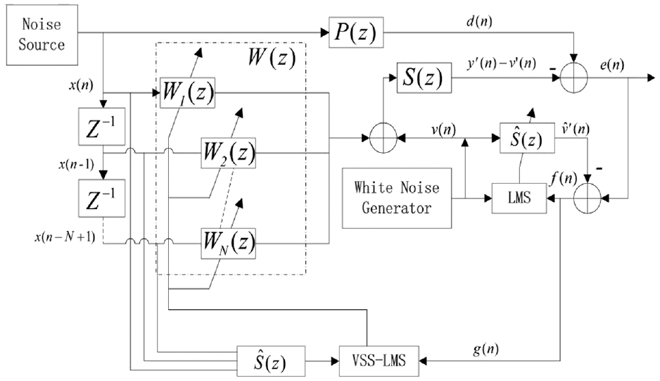
The optimization model based on Eriksson’s secondary-path online modeling system.
The optimization model based on Zhang’s secondary-path online modeling system.
Algorithm MATLAB simulation
In the following section, three different initial signals are substituted to verify the changes of the optimized model to the original model in different noise conditions. Where, the transfer function of the primary pathway is:
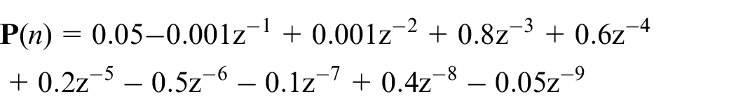
The transfer function of the primary pathway is:

Simulation of the random noise signal
The smooth noise signals are regarded as a reference signal to study the effect of noise suppression by various secondary-channel models of ANC. Figure 10 shows the smooth noise signals with a variance of 0.1.
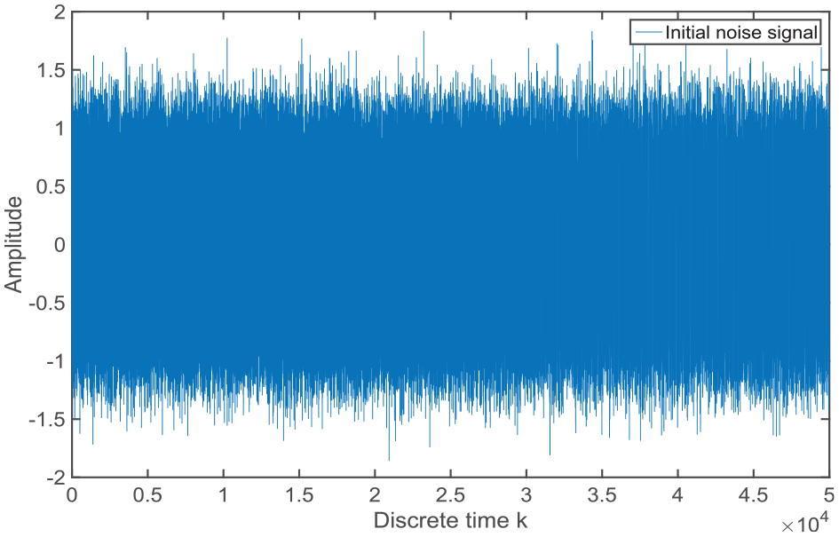
Initial noise signal l of steady fluctuation.
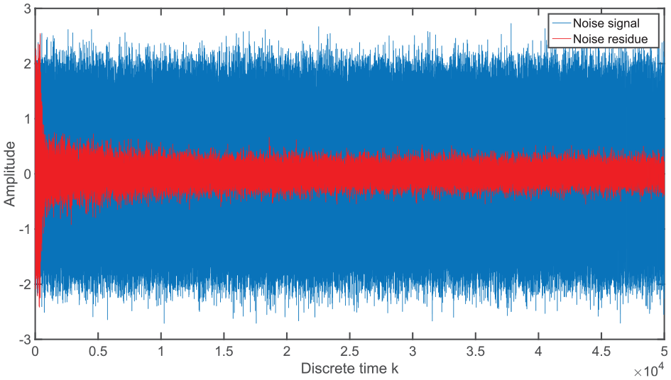
Figure 11 displays the noise reduction effect of Eriksson’s method. The blue line represents the original smooth noise signal, and the red line denotes the error signal obtained after inputting the secondary signal. In the initial time, the error signal sharply decreases and fluctuates slightly during a sudden change. Then it develops into stable fluctuation. The noise signals of using Eriksson’s method are lower than original smooth noise signals. Eriksson’s method can achieve a good noise reduction effect and reach stable fluctuation after convergence.

Noise reduction effect of Eriksson’s method.
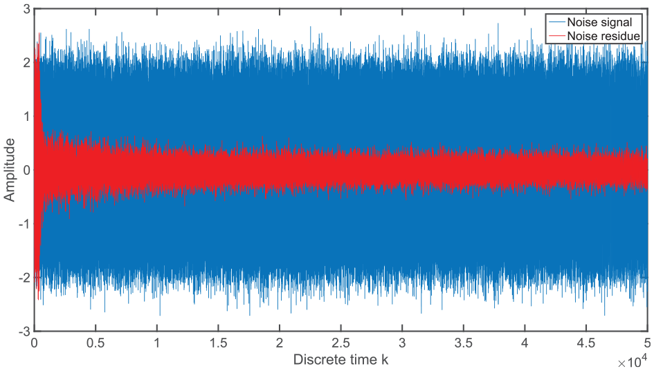
Similar to the noise reduction effect of Eriksson’s method in Figure 9, Zhang’s method and Akhtar’s method can reduce the noise signals compared with original smooth noise signals in Figures 12 and 13.
Noise reduction effect of Zhang’s method.
Noise reduction effect of Akhtar’s method.
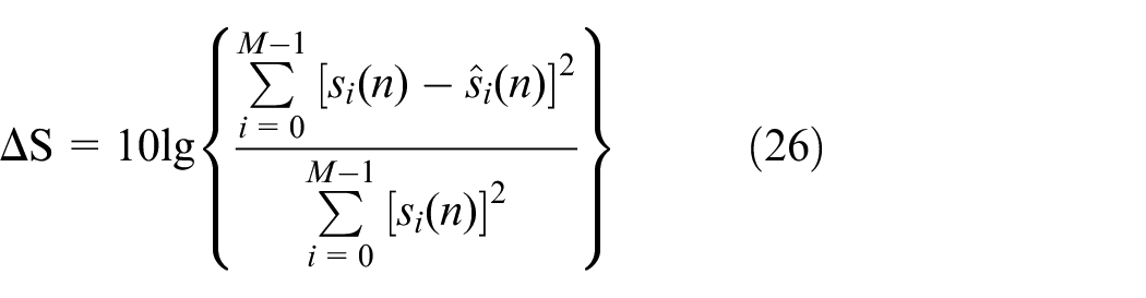
The measurement standard is defined as follows to measure the steady-state effect and noise reduction of the system.25–27

where
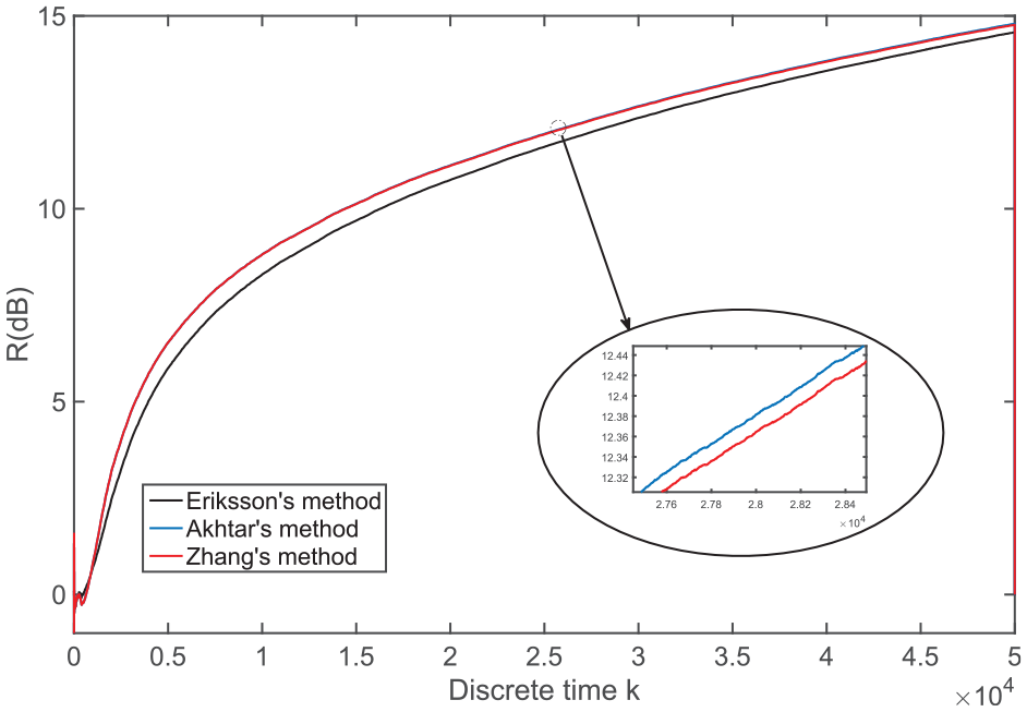
The three models mentioned above are substituted into the equation. Figure 14 shows the comparison of R-values in three previous schemes. The red, blue, and black lines represent Eriksson’s, Akhtar’s, and Zhang’s methods, respectively. R-value sharply increases in the initial stage and slowly increases in the middle and later stages. The noise reduction effect (R-value) of Zhang’s model is higher than that of Akhtar’s and Eriksson’s methods.
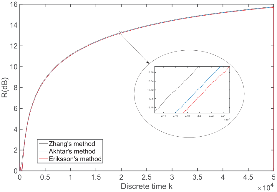
Comparison of R-values in three schemes.
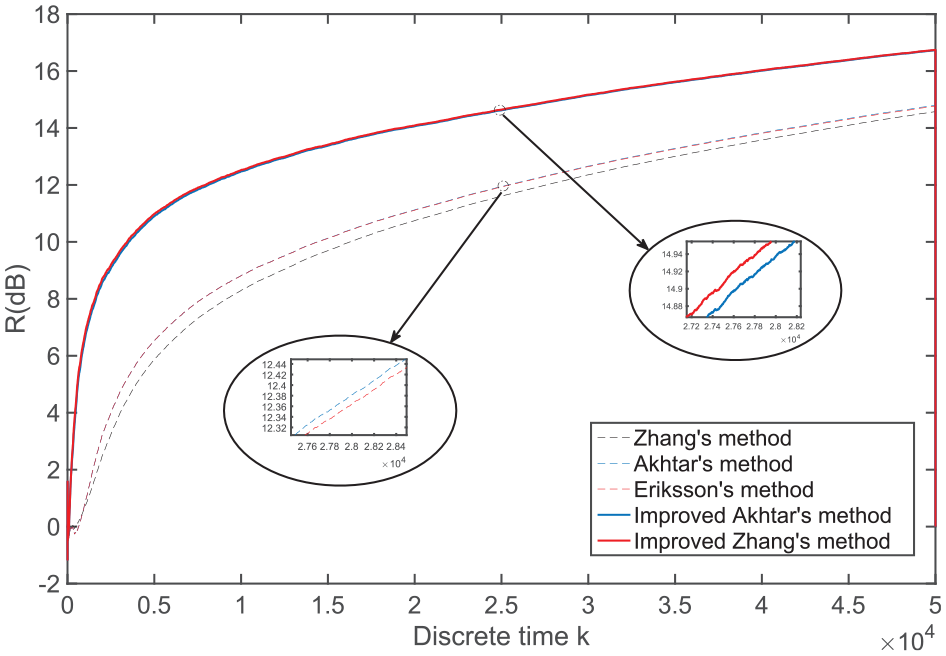
In Figure 15, the solid red and blue lines represent the noise reduction effects of the improved Akhtar’s and Zhang’s methods, respectively; the dotted line represents the values of three traditional schemes. The convergence speed and noise reduction effect of the improved Akhtar’s and Zhang’s methods are significantly higher than that of three traditional schemes in the discrete-time. Secondary-channel recognition error
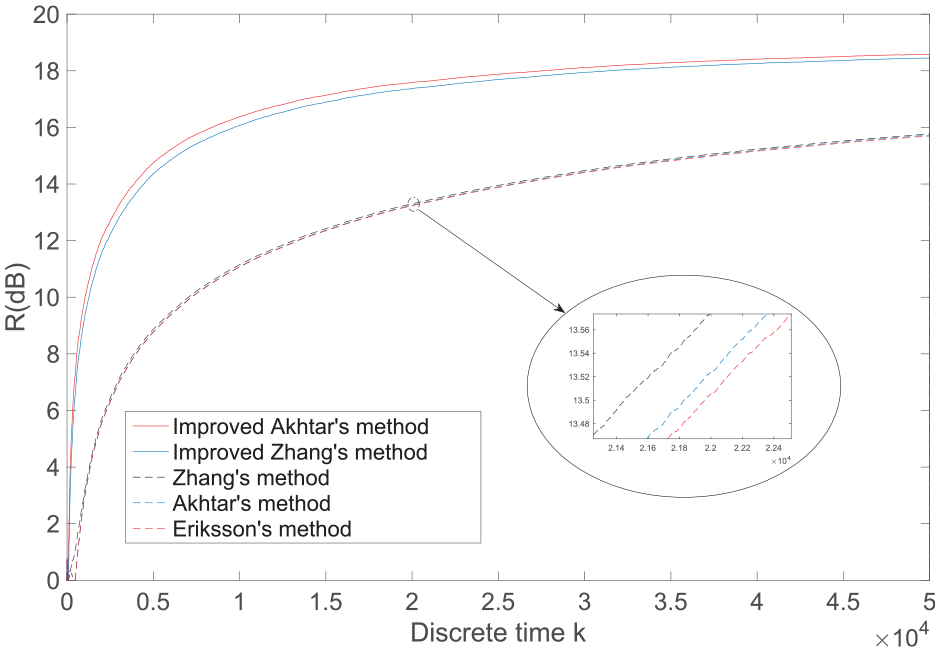
Comparison of R-values in three schemes and the result after introducing the improved algorithm.
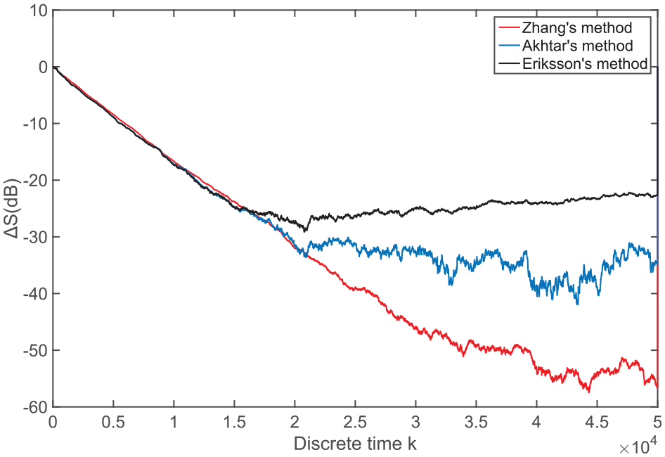
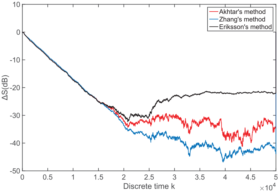
Similarly, the above three models are substituted into the equation. Figure 16 displays the comparison of ΔS values in the three schemes. The red, blue, and black lines represent Eriksson’s Akhtar’s and Zhang’s methods, respectively.
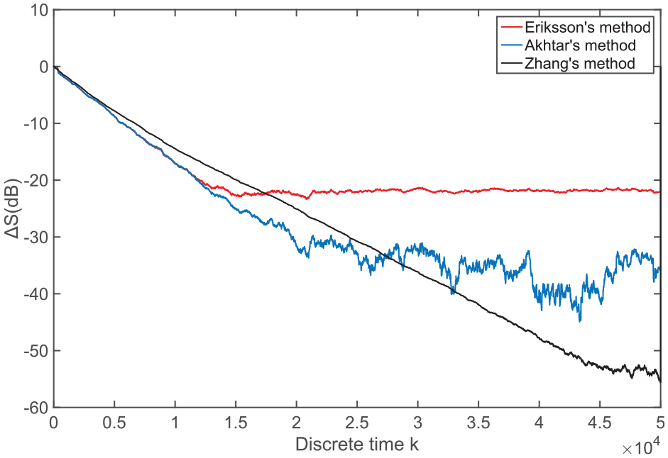
Comparison of ΔS values in the three schemes.
The convergence speed and fitting effect of the secondary-channel are judged by studying the falling speed and the minimum value of the curve. In Figure 16, Akhtar’s method can achieve better fitting of secondary-channel
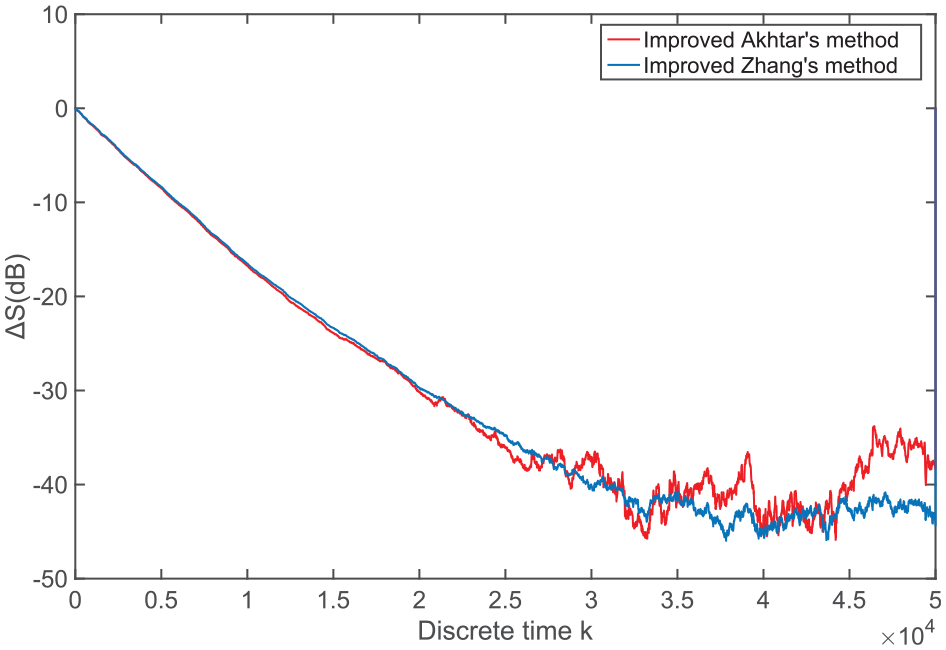
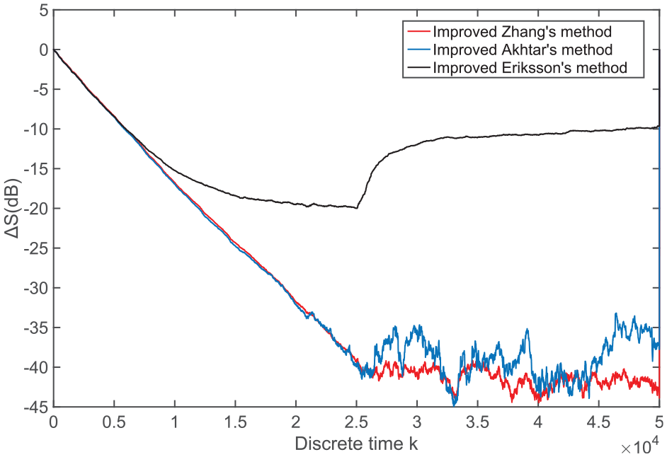
The two improved models are optimized by using the proposed algorithm. In Figure 17, the improved secondary-channel modeling has been significantly improved in convergence and fitting effects.
Comparison of ΔS values in the result after using the improved algorithm.
Simulation of the gradient noise signal
The initial noise signal of increasing signals is regarded as a reference signal to study the effect of noise suppression by the secondary-channel modeling of ANC, thus discussing the experimental effect under different initial signals. Figure 18 displays the initial noise signal of the increasing amplitude.
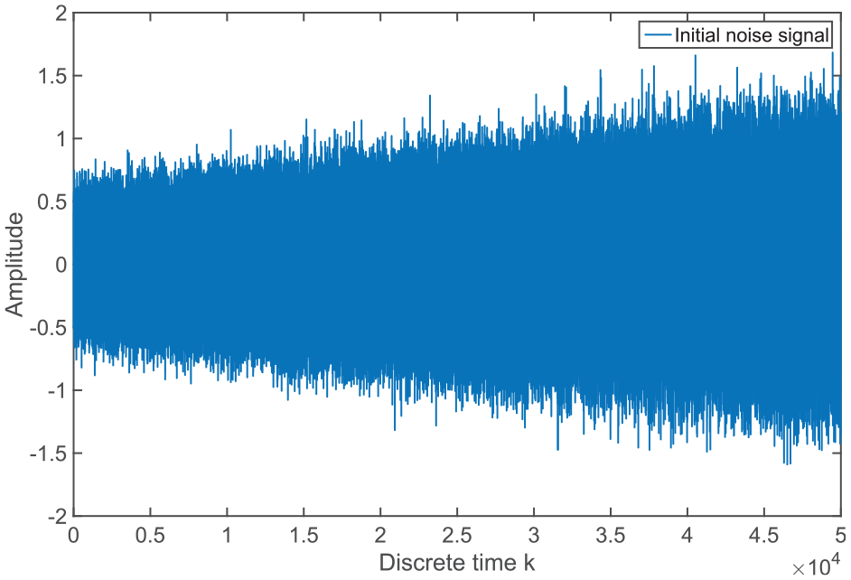
Initial noise signal of the increasing amplitude.
The set noise signals are substituted into the three initial models (Eriksson’s, Akhtar’s, and Zhang’s methods) to obtain the results in Figures 19 to 21.
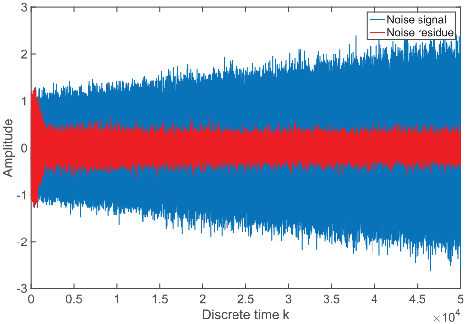
Noise reduction effect of Eriksson’s method with the increasing amplitude.

Noise reduction effect of Zhang’s method with the increasing amplitude.
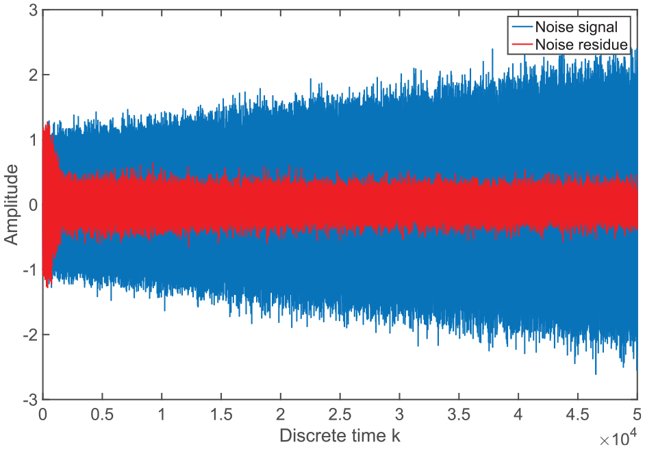
Noise reduction effect of Akhtar’s method with the increasing amplitude.
Figures 19 to 21 show that the three models can achieve a stable noise reduction effect under the gradient initial noise signal and fluctuate steadily within a certain range. The error is substituted into the formula to compare R-values (see Figure 22).
Comparison of R values in three traditional schemes.
Figure 22 shows the comparison among Eriksson’s, Akhtar’s, and Zhang’s methods. The noise reduction effects (R-values) of Akhtar’s and Zhang’s models are higher than that of Eriksson’s method with the discrete-time. R-value of Akhtar’s method is slightly better than that of Zhang’s method. Thus, Akhtar’s and Zhang’s methods are further extended to obtain a more effective noise-reduction effect.
In Figure 23, R-values gradually increase with the increased discrete-time, the convergence speeds and noise reduction effects of the two improved methods are higher than those of the three previous methods. Meanwhile, the noise reduction effect of the improved Zhang’s method is slightly higher than that of the improved Akhtar’s method.
Comparison of R-values among three traditional schemes and two improved algorithms.
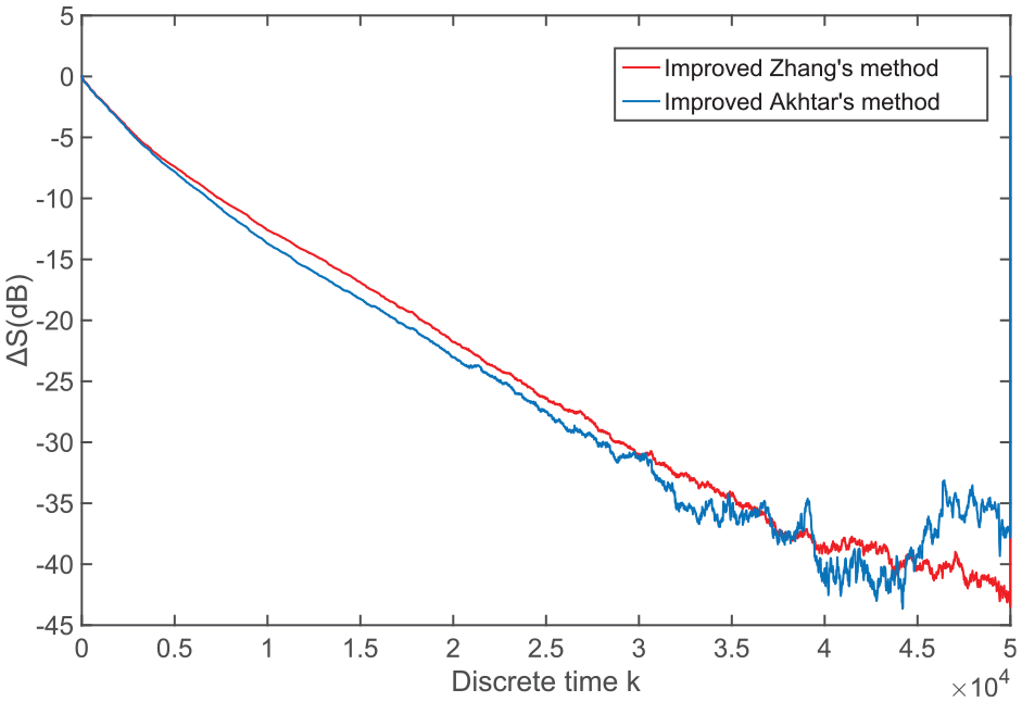
Comparison of ΔS values between Figures 24 and 25 shows that the improved Zhang’s and Akhtar’s methods can achieve a good fitting effect in the secondary-channel.
Comparison of ΔS values in three schemes.
Comparison of ΔS values in the result after using the improved algorithm.
Simulation of the abrupt noise signal
The abrupt noise signals are daily environmental noises. The abrupt noise signals are used to verify the modified models in the following subsection. Figure 26 shows the original abrupt noise signal for the test. When the discrete-time is 2.5, the amplitude of the noise signal sharply increases.
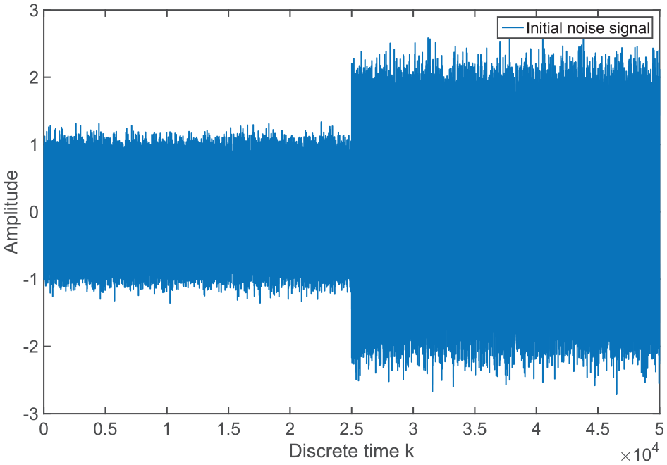
Initial abrupt noise signal.
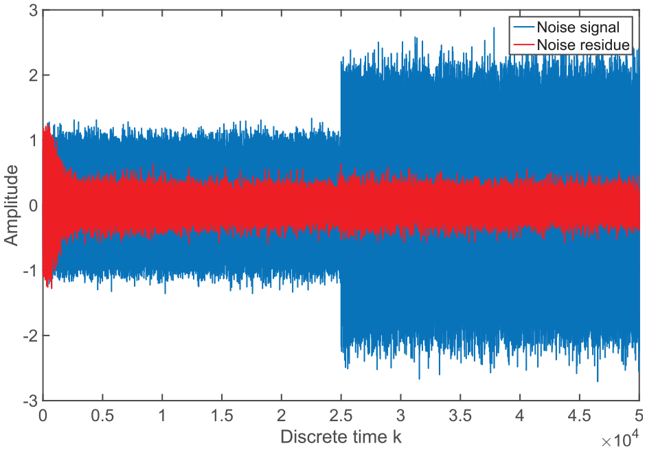
Figure 27 compares the noise reduction effect of Eriksson’s method. The blue line represents the noise signal obtained after the initial noise signal passes through the secondary-channel, and the red line represents the error signal obtained after inputting the secondary signal. The noise signals of using Eriksson’s method are low. The noise signals are suppressed using Eriksson’s method.

Noise reduction effect of Eriksson’s method.
Similar to the noise reduction effect of Eriksson’s method in Figure 17, the initial model has good anti-interference when the initial signal changes suddenly. The error signal fluctuates slightly and returns to stable fluctuation in Figures 28 and 29.

Noise reduction effect of Akhtar’s method.
Noise reduction effect of Zhang’s method.
The mutational initial signal is processed by more intuitive reflection through comparing R-values. In Figure 30, the black, blue, and red solid lines denote the R-values of Zhang’s, Eriksson’s, and Akhtar’s methods, respectively. R values gradually increase with time. R-value of Akhtar’s method is greater than that of Eriksson’s method.
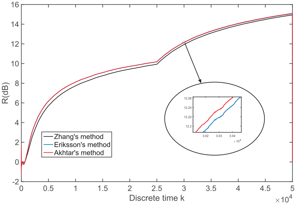
Comparison of R-values in the three schemes.
In Figure 31, the solid red and blue lines represent the effects of the improved Akhtar’s and Zhang’s methods, respectively; the dotted line represents the value before improving the three models. The convergence speed and noise reduction effect are optimized for the three improved models compared with those of the three traditional schemes.
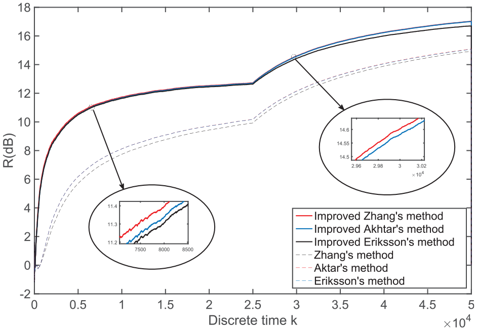
Comparison of R-values in three schemes and the result after using the improved algorithm.
Figure 32-33 compare the effects of secondary-channel modeling before and after the improved algorithm In Figure 32, the three original schemes have an approximate modeling effect, but Figure 33 shows that the improved Zhang and Akhtar’s methods have more effective convergence performance than that of Eriksson’s method. Fast and stable convergence performance of noise reduction for the improved Zhang and Akhtar’s methods is obtained in the fitting of the secondary-channel.
Comparison of ΔS values in the three schemes.
Comparison of ΔS values in the result after using the improved algorithm.
Conclusions
A new variable step size was proposed based on the logarithmic function of the Fx-LMS algorithm for secondary-channel online identification in the ANC system. The algorithm was used to optimize the step size of weight regeneration. The convergence speed and noise reduction of the ANC system were improved in the modified algorithm of ANC. The initial smooth noise signal, noise signal with the increasing amplitude, and abrupt noise signal were used to study the convergence speed and the noise reduction effect of the modified ANC method.
The results showed that the convergence speeds and noise reduction effects of the two improved methods were higher than those of the three previous methods. Meanwhile, the noise reduction effect of the improved Zhang’s method was slightly better than that of the improved Akhtar’s method.
Footnotes
Declaration of conflicting interests
The author(s) declared no potential conflicts of interest with respect to the research, authorship, and/or publication of this article.
Funding
The author(s) disclosed receipt of the following financial support for the research, authorship, and/or publication of this article: This work was supported by National Natural Science Foundation of China (11872337 and 11902291), Key Research and Development Program of Zhejiang Province (Grant No. 2020C01027) and Science and Technology Plan Project of Zhejiang Province (LGG21E060003), Natural Science Foundation Key Projects of Zhejiang Province (LZ22E060002), and the Science and Technology Key Plan Project of Zhejiang Province (2021C01049, 2020C04011).