Cough classification of MEMS microphone signal using time-series and tabular machine learning algorithms

Abstract

Cough is a protective mechanism of the proximal respiratory tract. The frequency and severity of cough provide useful information for the diagnosis of upper respiratory diseases and the evaluation of their treatments. Manual cough classification is subjective, labor-intensive, and time-consuming. In this study, a cough classification technique based on a microelectromechanical system microphone is proposed. For the classification process, various tabular and time-series machine learning algorithms were applied, and their results were compared. With respect to the time-series algorithms, the random interval decision tree, random interval spectral forest, and random convolution kernel transform (ROCKET) methods were used. With respect to the tabular algorithms, a convolution neural network (CNN) with 40 Mel-frequency cepstral coefficients (MFCCs) and a recurrent neural network with 40 MFCCs were used. Voluntary cough and noncough (throat clearing, expiration, speaking, and rest) signals were recorded from 10 healthy subjects. The ROCKET method showed the best accuracy (98.40%). In addition, while its training took the longest time (1628.80 s), this algorithm took a reasonably short time for prediction (0.27 s). The CNN showed the second-best accuracy (97.81%) with short training (454.13 s) and prediction (0.40 s) times. Thus, given its accuracy and prediction time, the ROCKET method is recommended for this type of classification over the CNN algorithm. To validate the application of the proposed methods, two methods were applied to a public Coswara data set. To classify one cough class and three non-cough classes, the ROCKET and CNN showed reasonable accuracies of 90.33% and 89.16%, respectively.

Introduction

Cough is a protective mechanism of the proximal respiratory tract. The frequency and severity of cough provide useful information for the diagnosis of upper respiratory diseases and the evaluation of their treatments. ¹ Conventionally, cough has been assessed manually, using methods such as cough visual analog scores and a diary scorecard. ² However, these methods have the limitation of being subjective. Nevertheless, the gold standard method for counting coughs is the manual counting of the cough sounds from near-patient audio recordings by an experienced expert. ³ However, this method is also subjective, as well as labor-intensive and time-consuming. Therefore, several attempts have been made to develop automated cough-detection techniques. Cough is known to consist of the following sequential stages: an inspiration state, during which air is drawn into lungs; a compression stage, during which the muscles cause forced expiration against the closed glottis; and, an explosive stage that accompanies the opening of the glottis and rapid air outflow. ³ This sequence provides several signals, such as voiced sound, chest wall motion, and airflow pressure. These signals can be captured by appropriate sensors and used to detect cough events. ⁴

Many studies have attempted automatic cough detection.^5–15 With regard to the sensor type, the majority of the studies have used audio sensors, such as audio microphones or contact microphones.^5,6 Birring et al. ⁵ collected cough signals from patients using an audio acquisition system called the Leicester Cough Monitor. They then used hidden Markov model algorithms to detect cough, achieving a sensitivity of 91.0% and specificity of 99.0%. ⁵ Drugman et al. ⁷ used multiple sensors, including an electrocardiogram, thermistor, chest belt, and accelerometer, for cough detection. After collecting voluntary cough and noncough signals from 32 healthy subjects, they achieved a sensitivity of 64.9% and specificity of 95.3% with an artificial neural network (ANN) classifier. Drugman’s group also used audio and thorax contact microphones and achieved a sensitivity of 94.7% and specificity of 95.0% with the ANN. Simou et al. ⁸ used a long-short term memory (LSTM) neural network model with heterogeneous datasets, achieving a sensitivity of 90.0% and specificity of 99.0%. Their heterogeneous datasets were unique, as they were collected from several online repositories. In addition, the LSTM model exhibits memory effects and thus shows reasonable performance, especially in the case of time-series data. Kruizinga et al. composed a training set of cough and non-cough sounds from various publicly available sources. They fit a Gradient Boost Classifier on the train data and validated on samples from 14 patients. They showed an accuracy of 99.6%, a sensitivity of 99.6%, and a specificity of 99.9% in the training set. The validation set results showed a sensitivity of 47.6% and a specificity of 99.96%. Abdelkhalek et al. used a convolution neural network (CNN) to detect coughs from publicly available data. They achieved a sensitivity of 92.7%, a specificity of 92.3%, and an accuracy of 92.5% using a sampling frequency of 750 Hz. Jokic et al. used a CNN with triplet network the situations that multiple individuals have to be monitored in shared environments. They applied this method to smartphone-based audio recordings from nocturnal coughs and asthmatic patients and showed a mean accuracy of 88.0%.

A few studies have used acceleration sensors. Mohammadi et al. ¹⁴ used cervical accelerometry, wherein an accelerometer is attached on the midline, below the laryngeal prominences, for cough detection. They used a binary genetic feature selection algorithm and a support vector machine classifier to achieve an accuracy of 99.3% in the discrimination of voluntary cough and rest accelerometry signals. Pahar et al. ¹⁵ applied a deep neural network algorithm with the results of bed-mounted accelerometer measurements and showed an area under receiving operator characteristic value of 0.98.

In general, two types of data are used in machine learning: tabular (or cross-sectional) and time-series. In the former case, the observational data samples are assumed to be independent and identically distributed (i.i.d.).^7–27 However, in the latter case, the order of the data samples carries intrinsic information. These tabular methods themselves show excellent performances in various fields of application such as healthcare and medical predictions. Although the LSTM algorithm is derived from an ANN and utilizes the characteristics of time-series data,^24,25 several algorithms, including those mentioned above, are tailored for tabular data. Recently, time-series machine learning algorithms have been introduced and are now being employed in various fields.^28–33

In this study, a cough classification method based on wearable audio signals is proposed. A microelectromechanical system (MEMS) microphone is used to realize a wearable sensor system. Several classification algorithms, including various time-series algorithms and conventional tabular data algorithms, are applied, and their results are compared. The proposed system was evaluated on healthy subjects from whom voluntary cough and noncough signals were recorded. The main contribution of this study can be summarized as follows.

• This study compares the suitability of several time-series machine learning algorithms for the classification of cough sounds.

• This study uses a compact MEMS microphone, which can be used as a wearable cough-detection device.

Materials and methods

Data acquisition system

To acquire the acoustic signals, sensor and processor boards were used (Figure 1). The sensor board (Adafruit I2S MEMS Microphone Break board, 16.7 × 12.7 × 1.8 mm³, Adafruit Industries LLC, NY) contained a MEMS microphone sensor (SPH0645LM4H, 18-bit, I2S, 3.50 × 2.65 × 0.98 mm³, Knowles, IL) to capture the acoustic signals. The processor board (Adafruit Feather M0 Adalogger, ARM Cortex M0 processor, 48 MHz, 51 × 23 × 8 mm³, Adafruit Industries LLC, NY) read the acoustic signals from the sensor board through an inter-integrated sound interface and sent the signals to a PC at 4000 Hz. The PC received the acoustic signals and saved them for analysis. The sensor and processor boards were connected to the power supply and the I2S interface using 1.5-m flexible wires.

Figure 1.

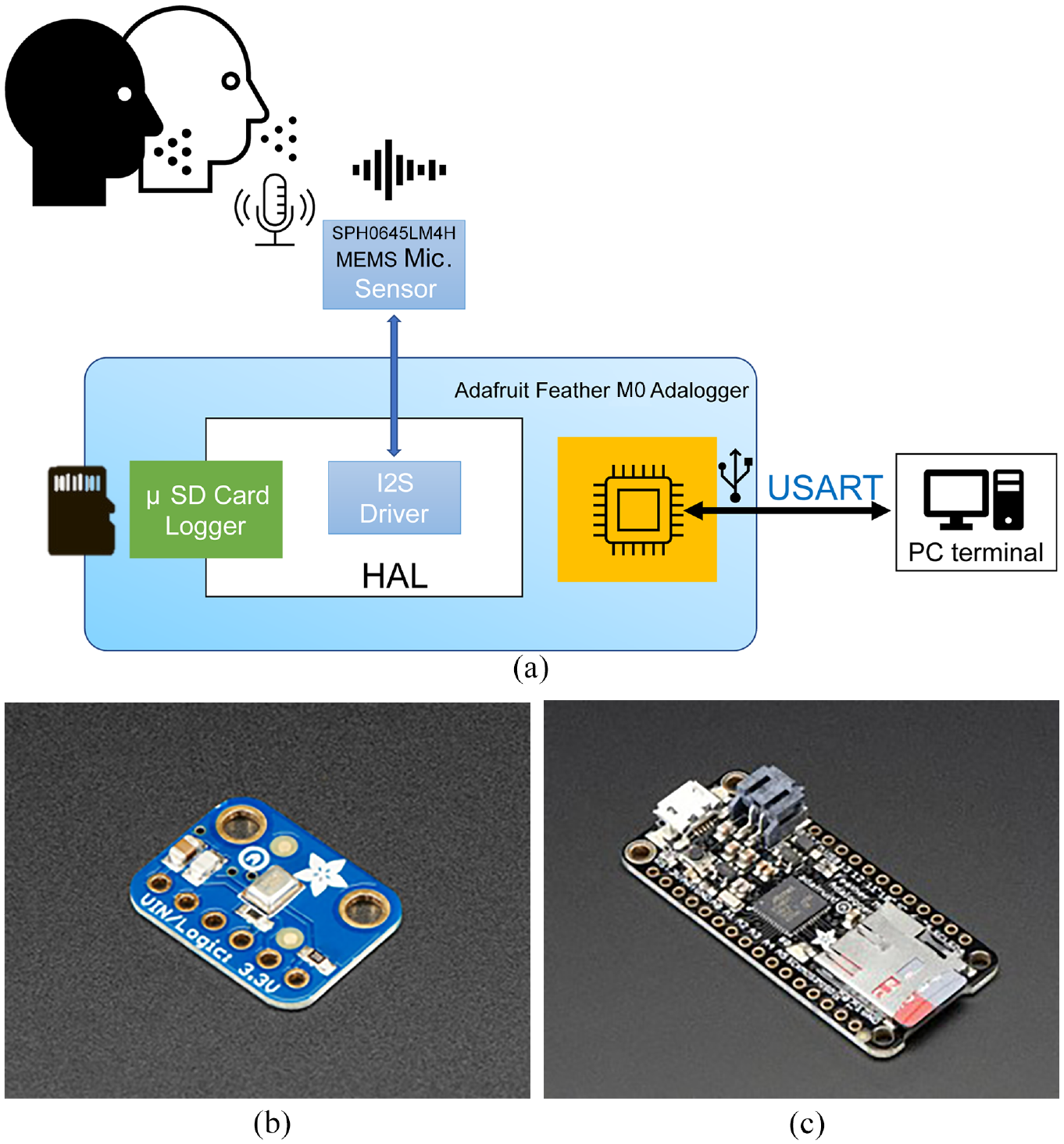
Data acquisition system: (a) block diagram, (b) MEMS microphone sensor, and (c) processor board.

Experimental protocol

The sensor board mentioned earlier was attached to the subject’s thorax (just below the suprasternal notch and on the body of the sternum), while the processor board was placed on a desk. The subject was made to sit on a chair during the experiment. Ten healthy subjects (four males and six females, mean age: 20.0 years, range: 22–26 years) participated in this experiment. All the participants provided written informed consent.

During the experiment, five classes of sound were captured: clearing the throat (“clear”), voluntary coughing (“cough”), expiration (“exp”), pronunciation of alphabet H (“h”), and resting (“rest”). For the first four classes of sound, the subjects made the corresponding sounds in response to a text display queue over 2 s. For the resting condition, the subjects were asked to stay calm for 2 s (Figure 2).

Figure 2.

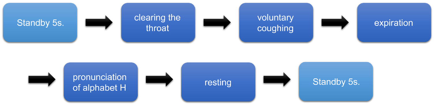
Block diagram of the experimental protocol.

Each type of sound was collected 12 times during a session. In addition, each session was repeated 10 times for each subject. Hence, 1200 sound samples were collected for each type, and a total of 6000 sound samples were collected for all the subjects and types.

Data segmentation

Each sound sample’s length was 8000 points, as the samples were collected for 2 s at 4000 Hz. Although the samples were segmented into 8000 points during the experiment, each sample was segmented once more into 3000 points as follows. First, the sound starting point was automatically detected based on the signal variation. Each variation over a sliding window with 2000 points was calculated (Figure 3 (bottom)). In this sliding window, the point at which the variation crossed over the maximum value was detected and considered the starting point of the sound sample. Then, the starting point was marked based on the sliding window size and backward 500 points margins. The ending points were calculated from the detected starting point and the fixed 3000-point length (Figure 3 (top)).

Figure 3.

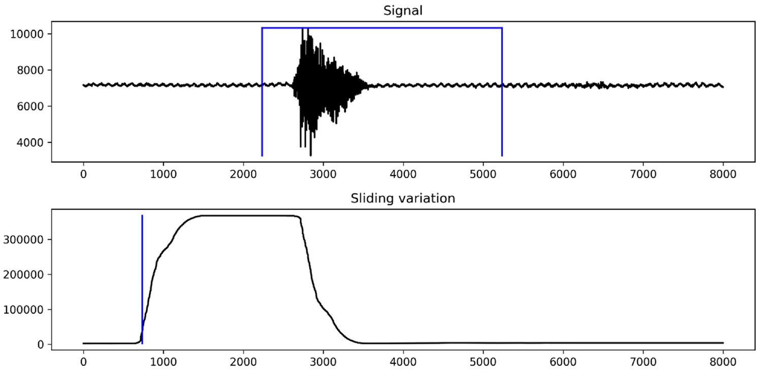
Sample segmentation: (top) sample signal with segmented area and (bottom) sliding variation.

Each segmented sample was plotted and checked by a person who did not participate in the experiment. Most of the samples could be segmented properly using this method. For the remaining ones, their starting points were determined manually.

Figure 4 shows typical example signals for the five classes. From the time-domain signals given in the top panes, it can be seen that the “clear” signal consists of a single burst of vibrations with a triangular shape. The “cough” signal rises sharply and then plateaus. The “exp” signal has a small amplitude but can be distinguished from the “rest” signal. Finally, the “h” signal consists of two consecutive bursts of vibrations. The frequency-domain shapes of the samples show that they have distinctive patterns. From these observations, it can be concluded that the time- and frequency-domain characteristics contain important information for signal classification.

Figure 4.

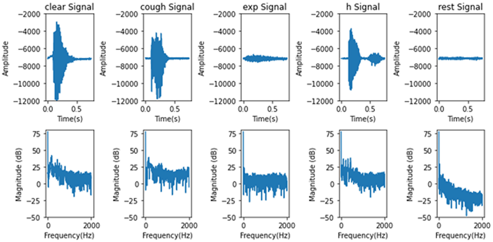
Example microphone signals: (from left on top) “clear,”“cough,”“exp,”“h,” and “rest.” Top and bottom panes correspond to time and frequency domains, respectively.

Tabularized time-series methods

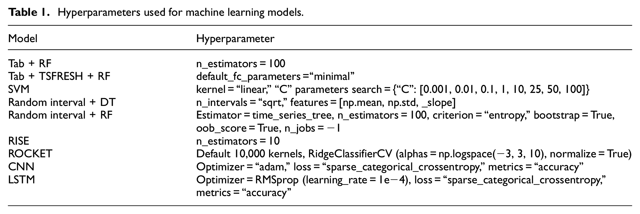
Tab + RF method: The simplest method for time-series classification is to convert the time-series data into tabular data (tabularization) and then analyze this converted data using a tabular method. In this case, the order of the time-series data samples was ignored, and the 3500 data points were assumed to be i.i.d. and treated as independent features. For the starting point, the random forest (RF) method was used. RF is an ensemble algorithm that averages the training performances of multiple decision tree (DT) models. The RF classifier creates a set of DTs from a randomly selected subset of the training set. It then aggregates the votes from the different DTs to decide the final class of the test object. The RF method is generally used as a baseline classifier for comparison with other algorithms. In this study, the “RandomForestClassifier” from “sklearn 0.0” Python package was used (n_estimators = 100). The hyperparameters are shown in Table 1.

Table 1.

Hyperparameters used for machine learning models.

Model	Hyperparameter
Tab + RF	n_estimators = 100
Tab + TSFRESH + RF	default_fc_parameters =“minimal”
SVM	kernel = “linear,”“C” parameters search = {“C”: [0.001, 0.01, 0.1, 1, 10, 25, 50, 100]}
Random interval + DT	n_intervals = “sqrt,” features = [np.mean, np.std, _slope]
Random interval + RF	Estimator = time_series_tree, n_estimators = 100, criterion = “entropy,” bootstrap = True, oob_score = True, n_jobs = −1
RISE	n_estimators = 10
ROCKET	Default 10,000 kernels, RidgeClassifierCV (alphas = np.logspace(−3, 3, 10), normalize = True)
CNN	Optimizer = “adam,” loss = “sparse_categorical_crossentropy,” metrics = “accuracy”
LSTM	Optimizer = RMSprop (learning_rate = 1e−4), loss = “sparse_categorical_crossentropy,” metrics = “accuracy”

The performance was validated with fivefold cross-validation. The entire data (6000 samples) were divided into five-folds (1200 samples for each fold, and 240 samples for each class) and iterated five times. For each iteration, four-folds (4800 samples) were used for training, and one-fold (1200 samples) was used for testing. The performances such as training time, prediction time, and accuracy were averaged for the five iterations. This fivefold cross-validation was used with the other methods as well.

Tab + TSFRESH + RF method: In this method, using the tabularized 3500 data points, nine types of features, such as the sum, median, and mean, were extracted. For this feature extraction process, the “tsfresh 0.10.0” Python package was used. ²⁹ With default_fc_paramter = “minimal” setting, features such as sum, median, mean, length, standard deviation, variance, mean square, maximum, and minimum were extracted.

DWT + SVM methods: In this method, DWT-derived features are extracted and fed into an SVM classifier. This type of method has shown excellent performances, especially audio classification including cough classification. ²⁴ DWT decomposes a signal into detailed coefficients using a wavelet kernel. The levels of detailed coefficients are carrying spectral information. SVM is well known to be calculation-effective and to show excellent classification performance. SVM seeks a hyperplane with boundaries that separate classes in an optimal way. In this study, approximate level and five-level detail coefficients were used. From each of these six coefficients, eight measurements (standard deviation, mean, root mean square, Shannon entropy, approximate entropy, permutation entropy, sample entropy) were calculated similarly to the reference 24. A total of 48 features were used for each sample. Daubechies-6 kernel was used for the wavelet.

Time-series methods

Random interval + DT method: First, this method splits the time-series data into random intervals with random start positions and lengths. Then, features such as the mean, standard deviation, and slope are extracted. Finally, a DT is trained on the extracted features. These steps are repeated until the required number of trees have been built or the time runs out. ³⁰

This process of feature extraction uses the order of the time-series to improve the performance with respect to the time-series data. The extracted features are then used with a DT classifier. The “RandomIntervalFeatureExtractor” from “sktime 0.7.0” Python package was used for the feature extractor (n_intervals = “sqrt,” features = [mean, std, _slope]). ²⁹

Random interval + RF method: In this method, multiple instances (100 in this study) of the random interval + DT method are ensemble-averaged. This ensemble is expected to improve the performance in the case of increased computation loads. The “ComposableTimeSeriesForestClassifier” from “sktime 0.7.0” Python package was used (estimator = time_series_tree, n_estimators = 100, criterion = “entropy,” bootstrap = True, oob_score = True, n_jobs = −1).

RISE method: The random interval spectral forest (RISE) is similar to the random interval + RF method. However, it uses a single time-series interval per tree and employs spectral features instead of the summary statistics. ³¹ In this study, the spectral features included the fitted autoregressive coefficients, estimated autocorrelation coefficients, and power spectrum coefficients. The “RandomIntervalSpectralForest” from “sktime 0.7.0” Python package was used (n_estimators = 10).

ROCKET method: The random convolution kernel transform (ROCKET) method randomly generates a wide range of convolution kernels and extracts two features for each convolution (the maximum and the proportion of the positive values) (Figure 5). ROCKET uses a large number (10,000 in this study) of different parameters (random lengths, dilations, paddings, weights, and biases) to capture the patterns corresponding to the different frequencies and scales. ³² For the classifier, the “RidgeClassifierCV” from “sklearn 0.0” Python package was used (alphas = logspace(−3, 3, 10), normalize = True).

Figure 5.

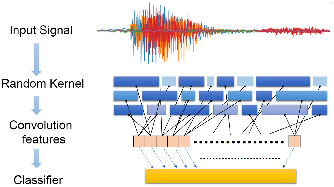
ROCKET model architecture.

ANN methods

CNN: The convolution neural network (CNN) is a deep learning algorithm model inspired by the biological structure of the visual cortex. The CNN is known to successfully capture the spatial and temporal dependencies in an image based on the use of various convolution kernels (filters). The CNN itself is designed for tabular data, including images. However, time-series data can be transformed into a tabular image and classified with a CNN.^16–18

In this study, two convolution layers were stacked and had 40 and 20 kernels. Both layers were max-pooled with a pooling size of 2 (Figure 6). After these two convolution layers, a dropout layer with a ratio of 0.4 was included to prevent overfitting during training. For the features, 40 Mel-frequency cepstral coefficients (MFCCs) were used with a window length of 1024 and hop length of 256.^34,35

Figure 6.

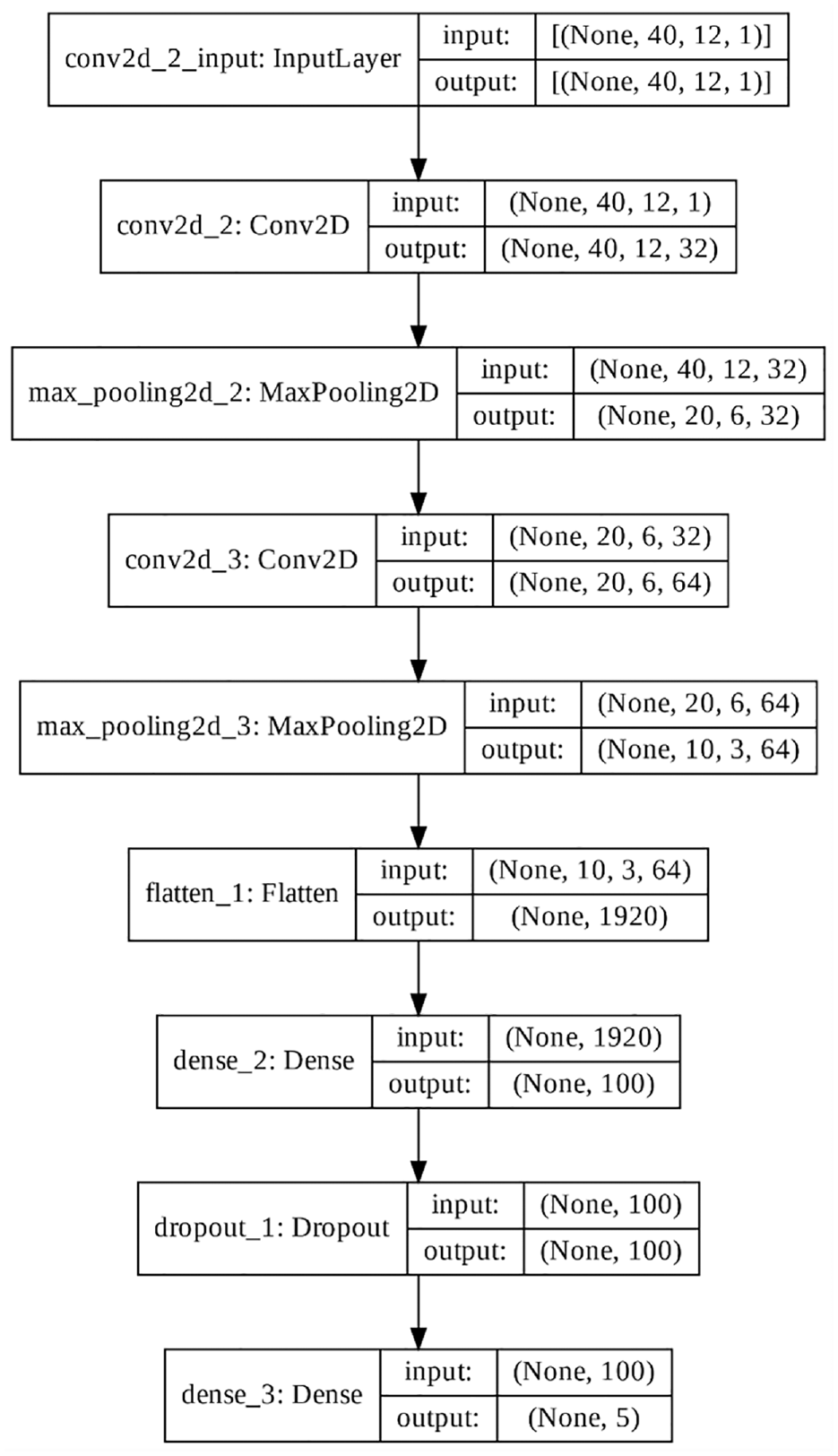
CNN model architecture.

The Keras 2.7.0 was used for the CNN (filters = 32 or 64, kernel_size = 3, activation = “relu,” padding = “same,” optimizer = “adam,” loss = “sparse_categorical_crossentropy,” metrics = “accuracy”).

LSTM: The LSTM is a recurrent neural network that takes the output of one neuron and returns it as the input to another neuron or feeds the input of the current time step to the output of the earlier time steps.^36,37 It has a memory, which enables it to remember important events that have happened many times in the past steps. The LSTM can handle gradients and disappearing problems, especially when dealing with long-term time-series data, and each memory unit (an LSTM cell) retains the same information about the given context.

In this study, two LSTM layers were stacked (Figure 7), and both layers had 100 units. After these two LSTM layers, a dropout layer with a ratio of 0.4 was added to prevent overfitting during training. For the features, 40 MFCCs were used with a window length of 1024 and hop length of 256.^34,35,38

Figure 7.

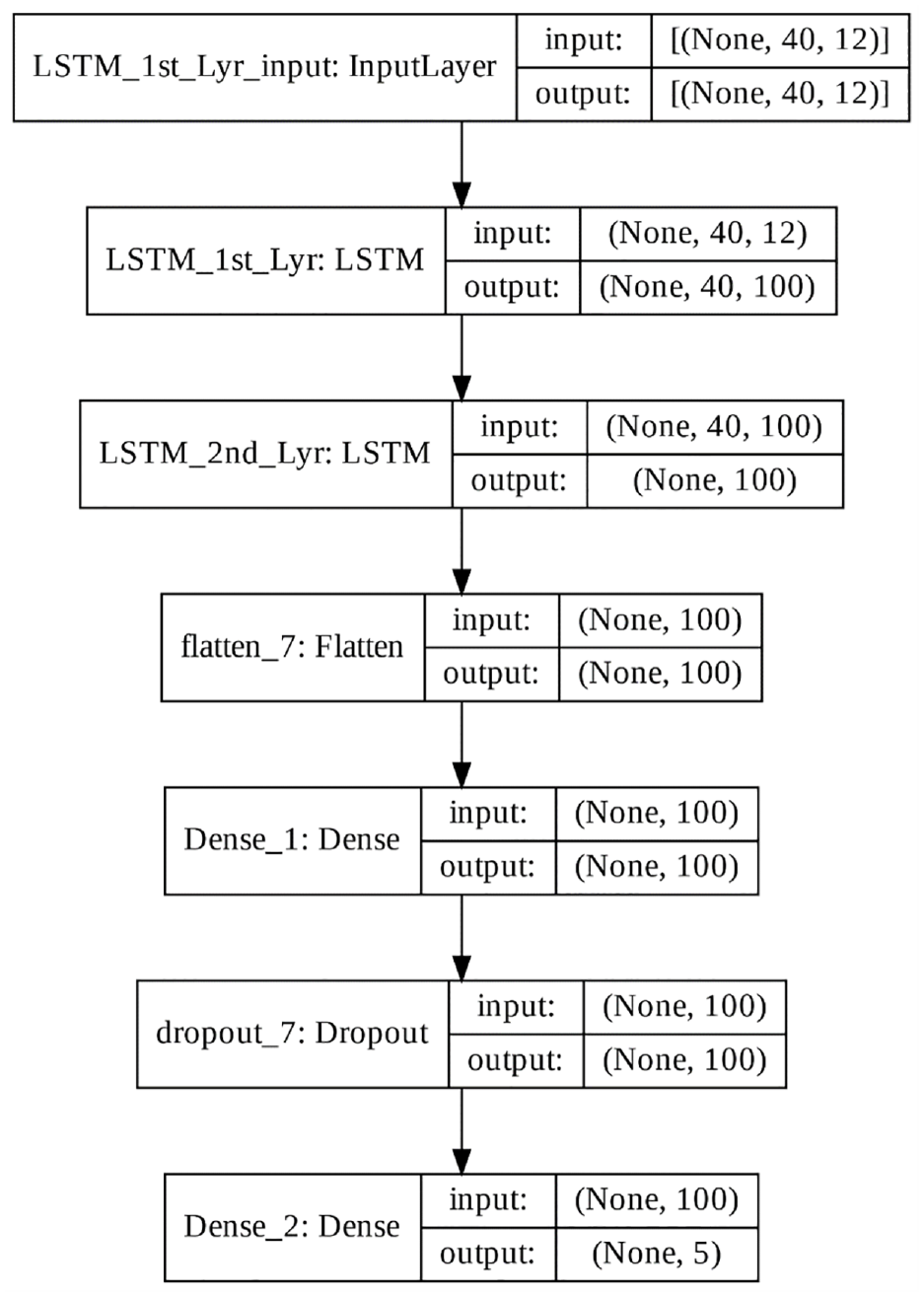
LSTM model architecture.

The Keras 2.7.0 was used for the LSTM (units = 100, optimizer = RMSpropm(learning_rate = 1e−4), loss = “sparse_categorical_crossentropy,” metrics = “accuracy”).

Results and discussion

The overall performances of the various algorithms used in this study are shown in Table 2. They are average values of fivefold cross-validation as described in the method section. The RF method with the tabularized features from the time-series data showed the lowest accuracies (84.05% for Tab RF and 83.70% for Tab + TSFRESH + RF). This seems reasonable because these algorithms ignore the order of time-series data. The Tab + TSFRESH + RF algorithm took less time for both training and prediction than did Tab + RF, as this algorithm uses the extracted features. In addition, the fact that the features extracted using the “tsfresh” package against the tabularized features resulted in lower accuracy highlights the importance of the time-domain information.

Table 2.

Performances of various algorithms (fivefold cross-validation).

Algorithm	Training time (s)	Test data prediction time (s)	Test data accuracy (%)	Precision	Recall	F1-score
Tab + RF	29.31	0.12	84.05	0.8424	0.8405	0.8405
Tab + TSFRESH + RF	1.23	0.04	83.70	0.8369	0.8370	0.8363
SVM	32.01	0.02	96.41	0.9642	0.9641	0.9641
Random interval + DT	5.68	0.88	83.62	0.8359	0.8361	0.8358
Random interval + RF	520.86	87.30	92.25	0.9230	0.9225	0.9223
RISE	285.20	68.60	88.55	0.8877	0.8855	0.8858
ROCKET	1628.80	0.27	98.40	0.9840	0.9840	0.9840
CNN	454.13	0.40	97.81	0.9785	0.9781	0.9781
LSTM	58.06	0.97	94.83	0.9487	0.9483	0.9482

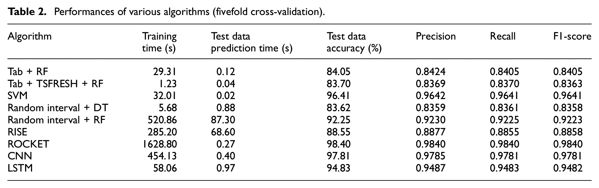
In the case of the time-series algorithms, the random interval + DT method showed no improvement in accuracy (83.62%). However, the random interval + RF method showed a significant improvement because of the ensemble effect (92.25%), although it took more time for training and prediction. The RISE algorithm showed no significant improvement (88.55%) and exhibited long training and prediction times. It can be assumed that the spectral data do not provide useful information in the case of time-series methods. The ROCKET algorithm showed the best accuracy (98.40%). However, its training took the longest time (1628.80 s), although its prediction time was reasonably short (0.27 s).

In the case of the ANN algorithms, the CNN method showed the second-best accuracy (97.81%) and short training (454.13 s) and prediction (0.40 s) times. The LSTM showed lower accuracy (94.83%) and shorter training (58.06 s) and longer prediction (0.97 s) times.

From these results, it can be concluded that the time-series algorithm ROCKET showed the best accuracy and the shortest prediction time, although it took the longest time for training. In addition, the CNN algorithm showed the second-best accuracy and a short prediction time.

Figure 8 shows the confusion matrices for the ROCKET and CNN algorithms for a specific fold. The ROCKET method confused “exp” and “h” more often compared with the CNN algorithm. However, the ROCKET method showed better discriminating performance in the case of the “clear,”“cough,” and “rest” signals. Moreover, these two algorithms showed different performance characteristics in the case of a few marginal cases. These complementary methods would likely exhibit better performance with respect to the marginal cases if used together.

Figure 8.

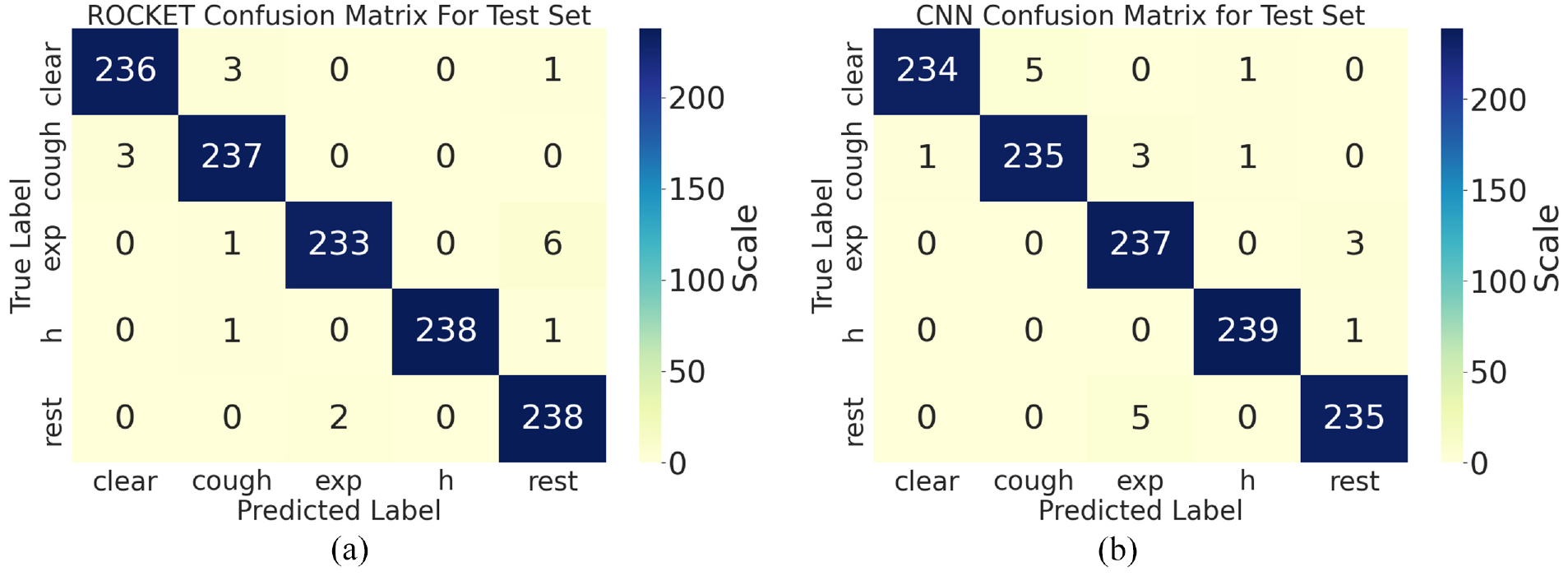
Confusion matrices: (a) ROCKET algorithm and (b) CNN algorithm.

Comparison with other techniques

The cough classification of this study shows comparable or superior performance compared with other state-of-the-art methods. To compare with other studies, we must convert our multi-class classification performance to binary classification performance. We merged the throat clearing, expiration, pronunciation of alphabet H, and resting samples to noncough samples for the specific result in Figure 8. Then we calculated the classification result of these noncough samples and voluntary cough samples. From this calculation, we got 99.33% accuracy, 98.75% sensitivity, and 99.47% specificity for the ROCKET method. The CNN method shows 99.16% accuracy, 97.91% sensitivity, and 99.47% specificity. This shows superior performance compared with other studies 91.0% sensitivity and 99.0% specificity, ⁵ 94.7% sensitivity and 95.0% specificity, ⁷ and 90.0% sensitivity and 99.0% specificity. ⁸ There was a study that showed 99.3% accuracy. ¹⁴ However, this accuracy is the performance to discriminate voluntary cough and rest accelerometry signals. In this study, no cough sample was classified as rest condition samples.

Performances on public data set

To validate the application feasibility of the proposed methods, two methods (ROCKET and CNN) were applied to a public Coswara data set. ³⁹ The Coswara is a crowd-sourced data set of sound recordings from COVID-19 positive and non-COVID-19 individuals. The volunteers provided nine audio recordings; shallow and deep breathing, shallow and heavy cough, sustained phonation of vowels (“e,”“ i,” and “u”), and 1–20 number counting (fast and normal paces). To compare our proprietary data set, four types of samples were used; deep breathing, shallow cough, fast 1–20 number counting. There are 2375 sets of samples in the Coswara data set. From these sample sets, sample sets that cannot be opened were excluded. Also, samples sets with a size shorter than 0.2 s were excluded. From the remained samples sets, 1200 samples set (48,000 samples over four classes) were randomly selected. Regarding the sampling rate, almost all of the samples were recorded at 48 kHz. For the comparison purpose, all the selected samples were downsampled to 4 kHz as in our proprietary samples. Also, regarding the duration, the samples in the Coswara data set have a duration of about 0.5–30.0 s. In this study, the duration was adjusted to 7.0 s. Samples with a shorter duration than 7.0 s were padded with the last sample point at the tails. Samples with a longer duration were cut in their tails. The ROCKET and CNN methods were applied to this prepared open data set. All the procedures were the same with the proprietary data set, including the hyperparameter and fivefold cross-validation.

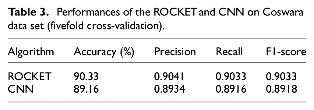
The fivefold cross-validation performances of the ROCKET and CNN methods on Coswara data set are shown in Table 3. Similar to the proprietary data set, the ROCKET method showed slightly better results. Both methods showed reasonable classification performance of about 90.0% accuracy, on a crowd-sourced data set.

Table 3.

Performances of the ROCKET and CNN on Coswara data set (fivefold cross-validation).

Algorithm	Accuracy (%)	Precision	Recall	F1-score
ROCKET	90.33	0.9041	0.9033	0.9033
CNN	89.16	0.8934	0.8916	0.8918

There is still a performance gap between the proprietary data set and the public data set. There could be several reasons for this gap. At first, from the nature of the crowd-sourced data set, there could be some data losses or low-qualified samples. Also, the single segmentation used in this case would not be efficient enough. Most of all, any optimization of model structure and parameters would be helpful.

Conclusions

In this study, a cough classification method for audio signals from a wearable MEMS sensor was proposed and evaluated. A MEMS microphone-based sensor board was attached to the subject’s thorax (just below the suprasternal notch and on the body of the sternum). Five classes (one voluntary cough class and four noncough classes) of sound samples were collected from 10 healthy subjects. In total, 6000 sound samples were collected and segmented for classification.

For the classification process, different tabular and time-series machine learning algorithms were applied, and their performances were compared. The RF method with the tabularized features from the time-series data showed the lowest accuracies (84.05% for Tab + RF and 83.70% for Tab + TSFRESH + RF). The Tab + TSFRESH + RF algorithm took less time both for training and prediction than did the Tab + RF method, as the former algorithm uses extracted features. The random interval + RF method showed a significant improvement owing to the ensemble effect (92.25%), although it took more time for both training and prediction. The ROCKET algorithm showed the best accuracy (98.40%), although its training took the longest time (1,628.80 s). However, it took a reasonably short time for prediction (0.27 s). The CNN method showed the second-best accuracy (97.81%) and short training (454.13 s) and prediction (0.40 s) times.

Thus, the ROCKET algorithm is recommended for this type of classification, based on its accuracy and prediction time, which were better than those of the CNN algorithm. Although the ROCKET algorithm took a long time for training, it would not matter in general cases, as the training would be performed once or infrequently if repeated.

To validate the application feasibility of the proposed methods, two methods (ROCKET and CNN) were applied to a public Coswara data set. The ROCKET and CNN methods on Coswara data set showed reasonable classification performance of about 90.0% accuracy, on a crow-sourced data set. There is still a performance gap between the proprietary data set and the public data set. This gap could be reduced in several ways such as checking the quality of crowd-sourced data, an advanced segmentation method, and optimization of model structure and parameters.

In future studies, the possibility of combining the ROCKET and CNN algorithms to complement each other and further improve the accuracy will be explored. In addition, the development of compact wearable cough-detection systems with cough sound processing and classification functions will be continued.