
Abstract
Previously, a nonlinear autoregressive network with exogenous input (NARX) demonstrated an excellent performance, far outperforming an established method in optimal baseline subtraction, for defect detection in guided wave signals. The principle is to train a NARX network on defect-free guided wave signals to obtain a filter that predicts the next point from the previous points in the signal. The trained network is then applied to new measurement and the output subtracted from the measurement to reveal the presence of defect responses. However, as shown in this paper, the performance of the previous NARX implementation lacks robustness; it is highly dependent on the initialisation of the network and detection performance sometimes improves and then worsens over the course of training. It is shown that this is due to the previous NARX implementation only making predictions one point ahead. Subsequently, it is shown that multi-step prediction using a newly proposed NARX structure creates a more robust training procedure, by enhancing the correlation between the training loss metric and the defect detection performance. The physical significance of the network structure is explored, allowing a simple hyperparameter tuning strategy to be used for determining the optimal structure. The overall detection performance of NARX is also improved by multi-step prediction, and this is demonstrated on defect responses at different times as well as on data from different sensor pairs, revealing the generalisability of this method.
Introduction
Guided wave testing is a commonly used non-destructive evaluation (non-destructive evaluation NDE) technique often applied to structural health monitoring (SHM), as in comparison to bulk wave inspections, it requires fewer sensors and less operator time in collecting test signals. This is because waves from permanently attached sensors can propagate over long distances in waveguides (e.g. plate-like structures and pipes). 1 The signals obtained from a network of sensors can be processed to form images to locate any defects in the inspected regions.2–4 In many structures, measured guided wave signals are dominated by the responses from structural features making the detection of responses from defects challenging. The general solution to this is based on recording one or more baseline signals when the structure is in a defect-free state, to which subsequent measurements can be compared. This forms the basis of a defect detection strategy for long-term monitoring called baseline signal subtraction.5–7 However, as the inspection may span multiple years during the lifetime of a structure, the changing environmental and operational conditions (EOCs), especially temperature, will distort the baseline signals of a defect-free structure. 8 These signals and their changes are complex, making it hard to distinguish real defect responses from those arising from changes in EOCs.
Various compensation techniques have been developed to reduce the effect of temperature on the baseline signal. This includes baseline signal stretching,9–11 optimal baseline selection (OBS),9,12 a combination of the two, 13 as well as more recent developments compensating for a range of effects besides the change in velocity.14,15 OBS, which selects the best matching baseline signal from a pool of signals, then amplitude stretched and time stretched, 13 has been compared to another data-driven approach, nonlinear autoregressive network with exogenous input (NARX), which is a machine learning (ML) method. The latter has shown superior defect detection performance. 16 Previous work with NARX 16 processed data spanning 8 years from a sparse array of permanently attached sensors on a steel tank. The network was trained using defect-free signals recorded when the structure was assumed to be pristine, and predicted baseline signals with matching EOCs when given synthetic defect test signals. The degradation of the tank over several years was assessed, and the defect detection performance of the network was further validated by introducing a physical anomaly to the tank. Other ML methods have been investigated for anomaly classification17,18; however, they require carefully designed example defect data for training.
The NARX network is an autoregressive neural network containing a single hidden layer that predicts a future point in a time-domain guided wave signal based on previous points (history) in the signal. The history points are repeated in a specific way to feed a wider input layer for the NARX network. This paper aims to improve the training robustness and physical interpretability of the network structure, by understanding how changing the length of history input, the width of the input layer and the number of future steps to predict ahead, affects its detection performance, using the same experimental data as previous work. 16 Subsequently, it aims to show the training procedure and detection performance of the network is robust to different initialisations of weights, defect responses at different times and data from different sensor pairs, revealing the potential of generalising such a network for similar defect detection problems in SHM and NDE.
The paper is organised as follows. Section 2 introduces the NARX structure, and Section 3 the data used for training, validating and testing NARX. In Section 4, the primary drawback of the previously implemented NARX is presented. Section 5 proposes an optimal network structure using a new approach to hyperparameter tuning. Section 6 shows that the new structure overcomes the drawback of the previous implementation, providing more consistent, better defect detection performance. Section 7 generalises the use of this network structure to different datasets.
NARX structure
In the current paper, NARX is implemented as a fully connected neural network with one hidden layer, which takes
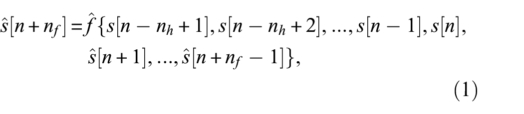
where
A flow chart illustrating the NARX implementation on time-series data is shown in Figure 1(a).
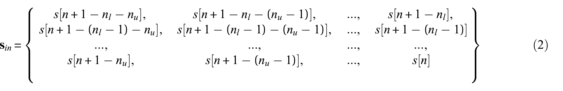
Therefore
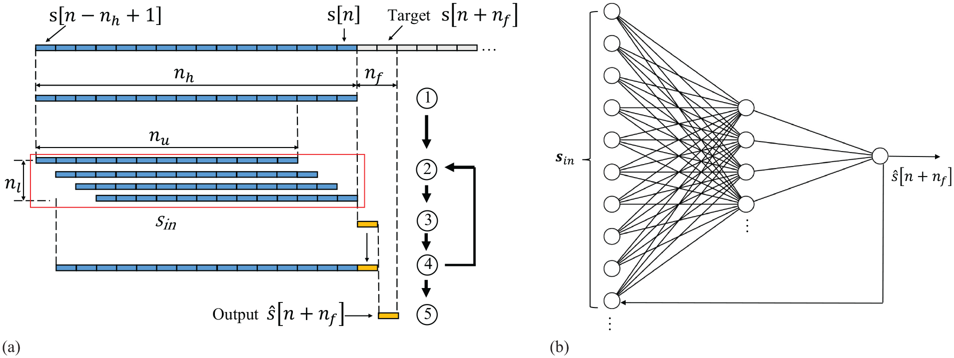
(a) Example flow chart of NARX implementation on time-series data. Blue indicates known values taken from data, and yellow indicates predicted values. (b) Schematic drawing of a NARX network.
The total number of weights and biases of the network is given by
Current work migrated the NARX network from Matlab to Tensorflow, as the latter provides greater capacity for processing large datasets and more flexibility in adapting network structure through lower level coding. This migration necessitates the use of a different optimiser, Adam, which is commonplace in Tensorflow, rather than Levenberg–Marquardt, the default for NARX in Matlab. The default learning rate of 0.001 was found to yield best performance. A batch size of 256 was found to be optimal among a range tested (from 32 to the training sample size). The network is trained to minimise the mean squared error (MSE) loss metric between
Data for training, validating and testing NARX
The experimental data consist of guided wave signals obtained from nine piezoelectric disc sensors permanently installed on a steel water tank, and monitored from 2012 to 2020, following the previous work. 16 The data from the years 2012 and 2013, which are the immediate measurements after sensor installation, are assumed to represent the tank’s pristine condition for the purposes of subsequent monitoring. The current work first investigated the NARX network in detail with data from one sensor pair: transmit on Sensor 1 and receive on Sensor 8. The training data are comprised of 20 signals chosen from the 2012 set over a relatively even distribution of EOCs. The validation data and defect-free test data are comprised of 5 and 200 signals from 2013. Later, more training data are added at random and data using different sensor pairs are also investigated.
The signals transmitted by the sensors are chirp excited,
22
and deconvolved to a five-cycle Hanning windowed toneburst with a centre frequency of 250 kHz,
16
and propagate primarily as
Artificial defect reflections, which are scaled and delayed tonebursts, were added to the defect-free test signals to form synthetic signals. Only one such defect response is added to each signal. This model is thought to be more conservative than the real measurements, because it ignores subsequent echoes and shadowing, which are likely to be bigger than the direct reflection from the defect. The defect responses were scaled to the time of the first arrival signal, referred to as the Syn1 method in previous work,
16
to simulate the beam spreading effect, and were multiplied by another scale factor, referred to as severity (given in dB),
16
to represent the size of the defect response. Therefore, the amplitude
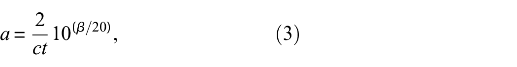
where
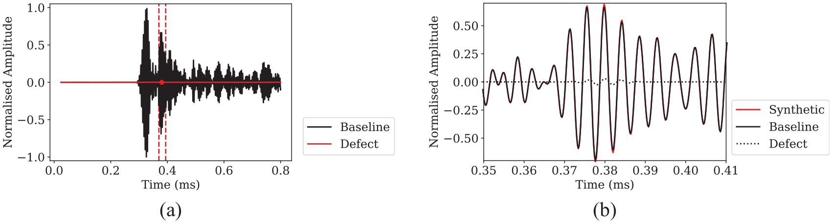
(a) Baseline signal and added defect signal of amplitude −30 dB. Red dashed line indicates the location of the defect in time. (b) Zoom-in of synthetic data at defect location.
A standard criterion is set to measure the performance of networks, a detailed description of which can be found in previous work. 16 The receiver operating characteristic (ROC) curve of each defect is computed using probability of false alarm and probability of detection (POD) at different detection thresholds. If the maximum amplitude of a defect-free residual signal exceeds a threshold, then it indicates a false alarm; if the maximum amplitude of a residual signal with defect exceeds a threshold, then it counts towards POD. The area under curve (AUC) is calculated for each ROC. Higher AUC indicates the detection performance for that defect is better. The lower limit of AUC is 0.5, equivalent to random guessing.
Shortcomings of single-step prediction
To understand the limitations of the existing approach, various training algorithms, learning rates, batch sizes and two different ML environments (Matlab following previous work
16
and Tensorflow) were investigated for the previous NARX structure:
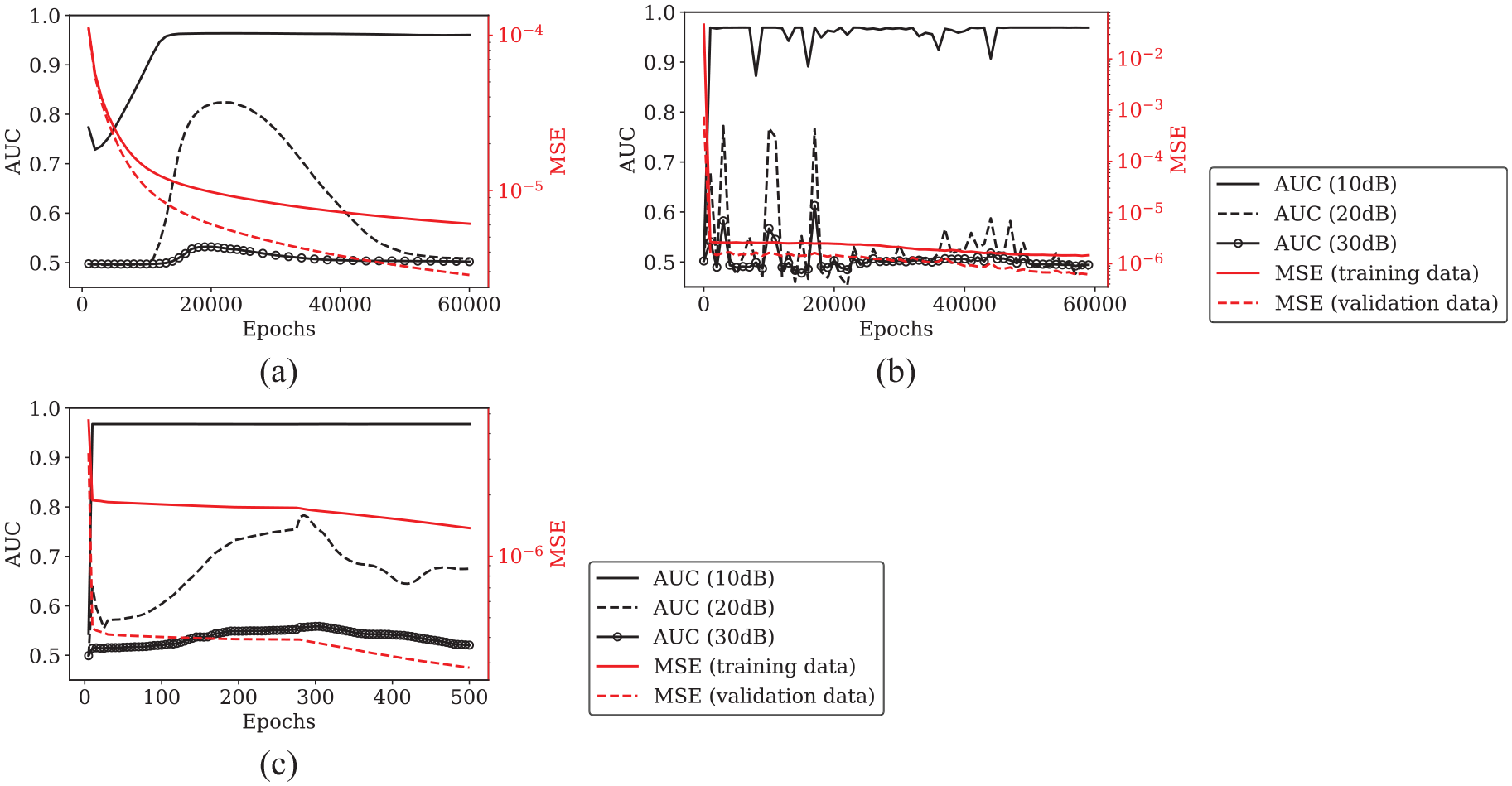
AUC, and MSE for both training and validation data evaluated over training history of single-step prediction NARX for training algorithm: (a) GDX in Matlab, (b) Adam in Python, and (c) Levenberg–Marquardt (default for NARX) in Matlab.
Increasing the correlation between MSE and AUC will improve the robustness of the training procedure, which is the main aim of this work. Validation loss is used as an indicator of how well the model will perform at its intended task: detecting defects in the test set. Although ultimately the detection performance is indicated by AUC, this is not suitable to be used as a loss metric – not only would this ramp up the computational burden, it would also require defect signals to be present in training data. This leads to difficult questions such as how big the defect should be, at what time should they occur, and are they representative of all possible defects of interest, etc, and bypasses the aim of defect-free model training.
Subsequently, multi-step prediction is investigated with the aim of reducing the disparity between the training loss metric, MSE, and the performance metric, AUC. It is believed that by predicting more steps into the future, the network will be unable to simply extrapolate forward as a way to reduce MSE between predicted and true signals. This means that when applied to a signal containing a defect response, the network should be unable to predict the defect response from data before it is visible in its input.
Hyperparameter study for multi-step prediction
This section searches for a network structure that can achieve excellent detection performance, which will subsequently enable the investigation of the AUC and MSE correlation for training robustness in the following sections. Therefore, a hyperparameter tuning strategy assisted by physical reasoning is presented, showing an efficient way to find an optimal structure without needing to test all possible combinations. Essentially, the performance of the NARX network is influenced by the following factors: how much history information is input to the network (
For the used digital time domain signals, it is more physically significant to describe
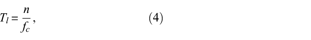
where
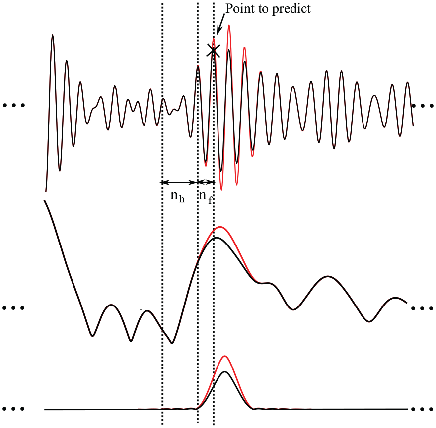
(Top) Extraction of data from an example baseline guided wave signal (black line) to be input to NARX network, and an example defect signal (red line) showing deviation from baseline signal where the defect occurs. (Middle) Signal envelopes of the example baseline and synthetic defect signal in the top graph. (Bottom) A simplified representation using only the envelopes of the windowed tonebursts at defect location.
Changing input layer width
This section aims to find the optimal combination of
To predict one cycle ahead,
Figure 5 plots the best AUC the network can achieve for detecting −30 dB defects in training history versus
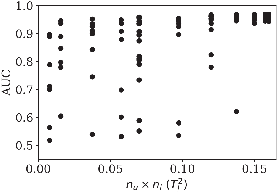
Best performance (AUC) the network can achieve throughout the training at different complexities with given history length
Changing future prediction length
The history length
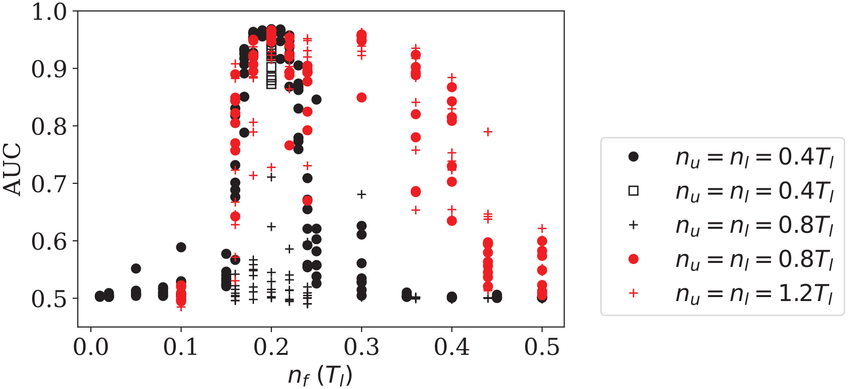
Best performance (AUC) the network can achieve throughout the training when predicting different points ahead. Results in black are from training data with 20 signals, results in red are from training data with 60 signals. Apart from results on black dots, all other results are obtained from down-sampled data.
Before more tests were carried out to see whether the network only performs best with the structure
Changing history length
Networks with increased history lengths are also assessed to determine the performance over different future prediction lengths to see whether the range for peak performances is extended this way. Both
On the other hand, increasing
To summarise, the peak performance around
Due to the presence of some abnormal measurements in the 2013 test data (4 out of 200 signals tested for sensor pair 1–8), the maximum AUC only reaches 0.97 in Figure 5 and 6. Those abnormal signals can be clearly identified from the test data, as their amplitudes are one order of magnitude lower than others. It is believed that these are a result of occasional poor electrical contacts in the relay-based multiplexors used to acquire experimental data from the array of sensors. The network can still distinguish the defects from noise in those residuals; however, a different threshold is required as the residuals are significantly lower than others, limiting the maximum AUC to below unity. The abnormal signals are omitted from the test data in subsequent sections to present the true detection performance of the network.
Repeatability of proposed NARX structure
The training metric, MSE of validation data, can be used as a good proxy for the desired performance metric, AUC, provided there is a strong correlation between the two. Therefore, this correlation is investigated using a training history of the proposed optimal structure of multi-step prediction NARX. AUC, and MSE for training, validation and test data are evaluated every 100 epochs, giving 80 checkpoints throughout training, which are plotted as training curves in Figure 7(a). The MSE of validation data is then plotted against AUC on a log scale in Figure 7(b), showing a clear monotonic trend – as MSE decreases and AUC improves. In contrast, log(MSE) against AUC for single-step prediction in Figure 7(c) (with values from training graph in Figure 3(b)) shows a lack of correlation, which explains why training lacks robustness.
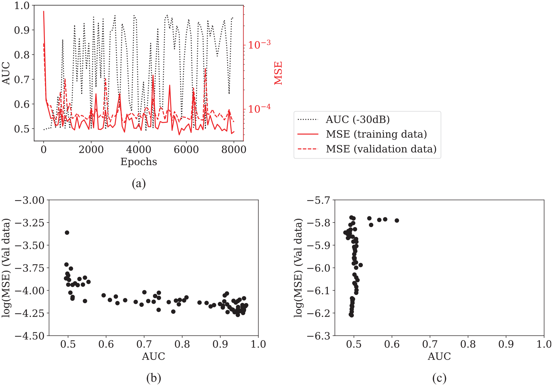
(a) AUC, and MSE for training, validation and test data evaluated at every 100 epochs over the training history of a multi-step prediction NARX with optimal structure
The Spearman correlation coefficient,
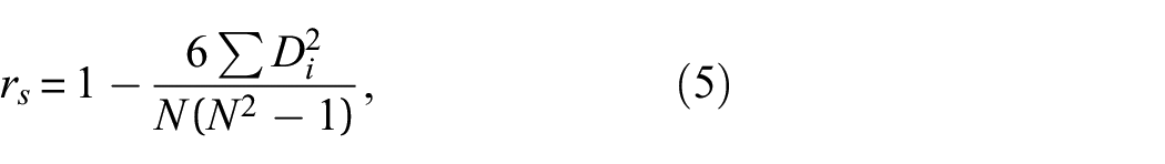
where
On this basis, the point of lowest MSE of validation data in training history in general leads to a network with good detection performance. Therefore, the multi-step prediction network with the optimal structure found in the previous section,
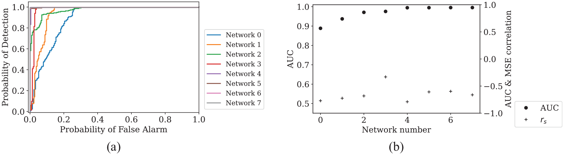
(a) ROC for detecting −30 dB defects by best performing networks trained with eight different initialisations. Networks saved at the point of lowest validation loss (MSE of validation data). Networks are ordered by detection performance from low to high. (b) Left axis: calculated AUC from the ROC curves. Right axis: Spearman correlation coefficient,
The multi-step prediction NARX network also demonstrates improved detection performance when tested with defects occurring at different times compared to the previously implemented single-step prediction network (Figure 9(a) and (b)). From the perspective of signal processing, single-step prediction gives unevenly distributed noise in the residual signal when subtracted from defect-free test data, as shown in Figure 10(a) and (b). Multi-step prediction with the optimal hyperparameters found in Section 5, on the other hand, gives more evenly distributed residual signal (Figure 10(c)). They can also maintain a good SNR when subtracted from test data with defects (Figure 10(d)), even though the average residual is much higher than that of single-step prediction networks (Figure 10(a) and (b)). The residual amplitude at the defect location is also more physically representative, as the defect in this case has an amplitude of 0.025 above the average residual. Comparing to its true amplitude of 0.027, this means defect responses are passed through the network largely unaffected. In other words, multi-step prediction with the optimal structure enhances the correlation between AUC and MSE and achieves good detection by reducing the occurrence of large values in the residual.
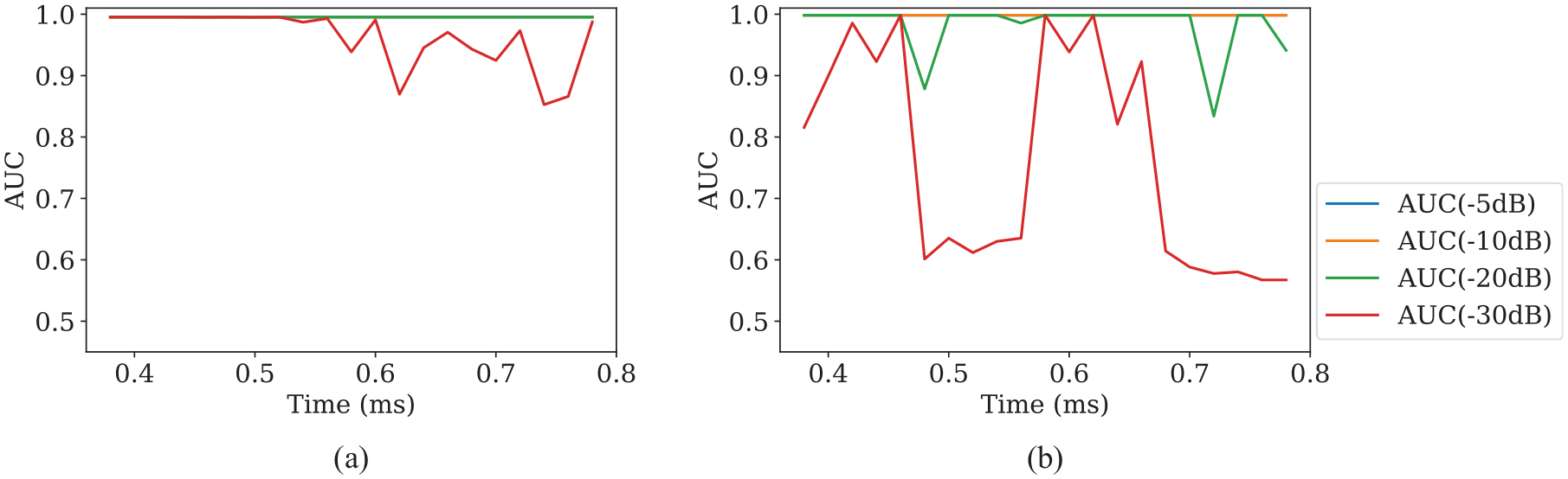
(a) Detection performance of multi-step prediction NARX with optimal structure
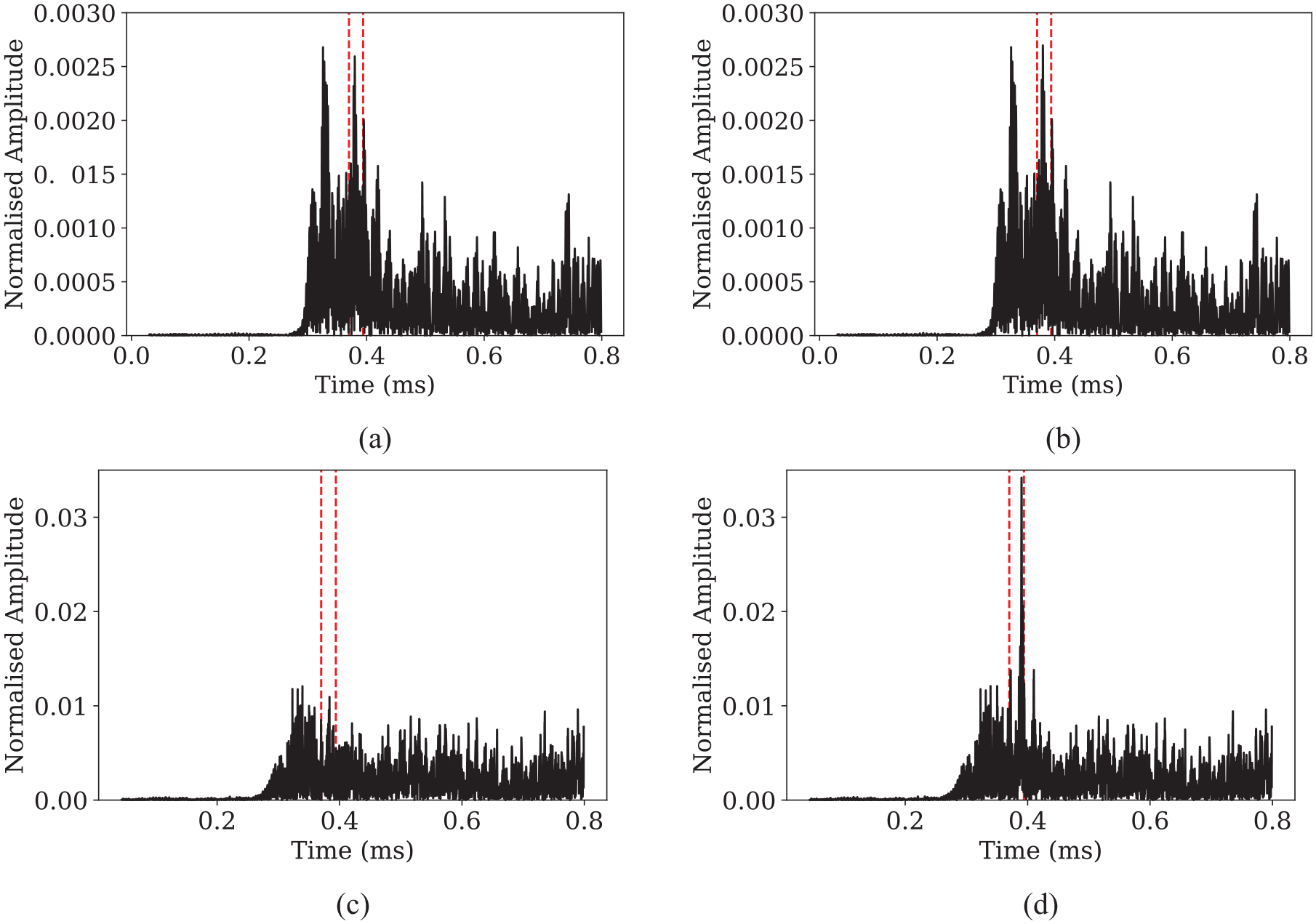
Residual signal from single-step prediction NARX (a) without defect (b) and with defect. Residual signal from multi-step prediction NARX with optimal structure (c) without defect (d) and with defect.
Generalisability of proposed NARX structure
The proposed optimal network structure,
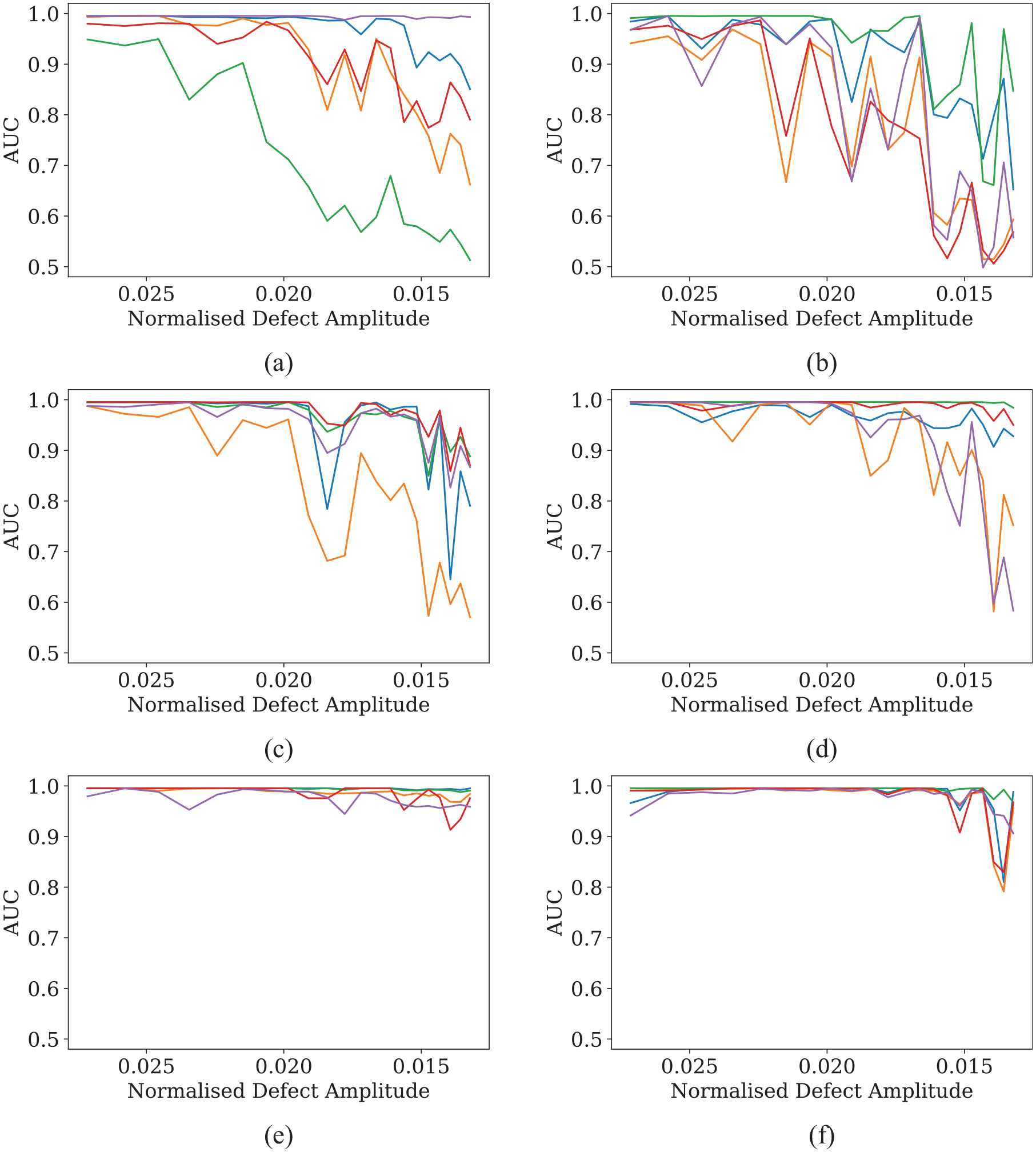
Defect detection performance of proposed optimal NARX structure trained and tested with data from (a) sensor pair 1–2, (b) sensor pair 1–3, (c) sensor pair 1–4, (d) sensor pair 1–5, (e) sensor pair 2–4 and (f) sensor pair 2–5. Defects appearing later in time are detected with smaller amplitudes due to beam spreading, so the x-axis ‘Normalised Defect Amplitude’ decreases from left to right. It follows the same direction of time as in Figure 9.
Conclusion
In this paper, the single-step prediction NARX network is found to have inconsistent defect detection performance, because the loss metric for training, MSE, is not a reliable indicator of the performance metric, AUC. By predicting multiple steps ahead, the NARX network is able to achieve a strong inverse correlation between MSE and AUC. This enables a robust training procedure to be defined, and the best performing network can be reliably selected from training history at the point of lowest MSE. The overall detection performance of multi-step prediction is also seen to be better than single-step prediction. This method is generalisable for data from different sensor pairs.
It is shown that by looking at the physical significance of the network with regard to the guided wave signals, a simple hyperparameter tuning for the optimal structure can be performed. This involves starting with a reasonable value of input history length based on a physically representative future prediction length, and then testing different future prediction lengths using the maximum network complexity for the given input history length. The input history length and the training set size should be increased when predicting further ahead.
Current work also reveals some questions that are worth future investigation, for example, how to quantitatively assess the effect of adding more input history length and training data, and where the upper limits of performance lie.
Footnotes
Acknowledgements
Declaration of conflicting interests
The authors declared no potential conflicts of interest with respect to the research, authorship and/or publication of this article.
Funding
The authors disclosed receipt of the following financial support for the research, authorship and/or publication of this article: The work reported is a continuation of a pilot project (grant no. 100374) originally supported by Lloyd’s Register Foundation and the Alan Turing Institute Data-Centric Engineering Programme.