
Abstract
The six-degree-of-freedom (6 DOF) motion of the mother-ship, which is caused by wave fluctuation, makes offshore operations difficult. To solve this problem, various heave compensation systems were proposed, as well as the law of wave motion. These heave compensation systems included passive heave compensation system, semi-active heave compensation system, and active heave compensation (AHC) system. However, the empirical formula of wave motion is not suitable for practical offshore operations, and rare AHC systems take the characteristic of compensation into consideration. To study the compensation characteristic of the AHC system based on electric-driven marine winch in the actual sea condition and improve the accuracy of compensation, this work uses the measured data of wave motion, and deduces the motion equations of multi-axial driving system. By substituting the above elements into the AHC system and designing the sliding mode controller (SMC), the simulation results show the ideal compensation effect of the system. By comparing with experimental results, it is concluded that the driving system operates in according with the specified states, and the compensation performance of system is effective. The overall work is conductive to the research on AHC system, as well as the exploitation of marine resources.
Introduction
The marine winch is an important marine equipment installed on the mother-ship, and it is usually used for hoisting and recycling operations. For example, it has been widely used in offshore pipeline laying, replenishment between ships and other fields.1,2 However, the wave fluctuation makes the mother-ship present a six-degree-of-freedom (6 DOF) motion, such as roll, pitch, and heave.3,4 The 6 DOF motion generally affects the operating accuracy of marine winch seriously, and even causes the cable to be broken.5,6 When the marine winch works, AHC technology plays a major role in reducing the impact caused by wave fluctuation. The existing researches on AHC technology generally take simplified sinusoidal wave as external excitation, while most objects of compensation are hydraulic-driven winches.7,8 In other researches, for example, Do and Pan 9 proposed a heave compensation system for hydraulic-driven double-link actuator, which estimated the force between the drill string and AHC unit. Gunvaldsen and Gunvaldsen 10 developed a dynamic simulation model for an AHC system. Richter et al. 11 used trajectory planning algorithm to compensate load displacement, while the object of compensation was a hydraulic-driven winch. Liu et al. 12 developed a suite of software programs to enable real-time monitoring of the dynamics of logging tools, and assessed the efficiency of wireline heave compensation during downhole operations. To reduce the adverse effect of unexpected vessel heave variation on the response of the underwater payloads, Li et al. 13 designed a hybrid active-passive heave compensation system with a nonlinear cascade controller. Richter et al. 14 proposed a real-time model predictive trajectory planner for an AHC system. Küchler et al. 15 proposed a prediction algorithm for the vertical motion of the vessel and formulated an inversion-based control strategy for the hydraulic-driven winch. Li et al. 16 designed a nonlinear controller and combined with sliding mode controller to compensate the heave fluctuation of load under 3–4 level sea condition. Cuellar and Fortaleza 17 proposed a hydro-pneumatic heave compensator and a semi-active control method. Zhang et al. 18 studied the semi-active drill string and established the mechanical model of a heave compensation device.
Compared with hydraulic-driven methods, the electric-driven system has the advantages of effectiveness and convenience in controlling the system. Meanwhile, the AHC system has a higher compensation rate than that of the semi-active heave compensation system. For above reasons, this work uses the electric-driven marine winch with AHC technique as the compensator. On the one hand, most researches ignore the complexity of wave motion and simplify the wave motion, making this simplification unable to reflect the reality. On the other hand, although the research on AHC has been a major topic for discussion in recent years, rare AHC researches have taken the detailed working states of driving system into consideration. Therefore, this work adopts the inertial measurement unit (IMU) to collect the data of heave displacement, and uses its expression in time domain as the external excitation of simulation model. Furthermore, the modeling of the AHC control system for the electric-driven marine winch has been completed. In this part, not only the working states of driving system have been considered,19–21 but also the corresponding controller has been designed. Finally, this work has carried out the experiments on land to verity the system modeling. These works make the research more practical and meaningful to a great extent.
System mathematical model
Figure 1 shows the process of heave compensation, and the marine winch connects the load through the rope. Generally, it is supposed that the load locates at the expected location in offshore operations. However, with the influence of wave fluctuation, the load usually puts out of its expected location. In this case, the heave compensation system adjusts the length of rope to keep the load at the required position. The AHC system discussed in this work consists of mother-ship, marine winch, three-phase asynchronous motors, programmable logic controller (PLC), IMU, cable, and equipment, Figure 2 shows the structure diagram of it. According to the principle of feedback control, IMU detects the real-time sea condition, PLC handles such information and outputs signals for controlling motor speed and rotary direction to the frequency converter, so as to drive the winch drum to rotate.
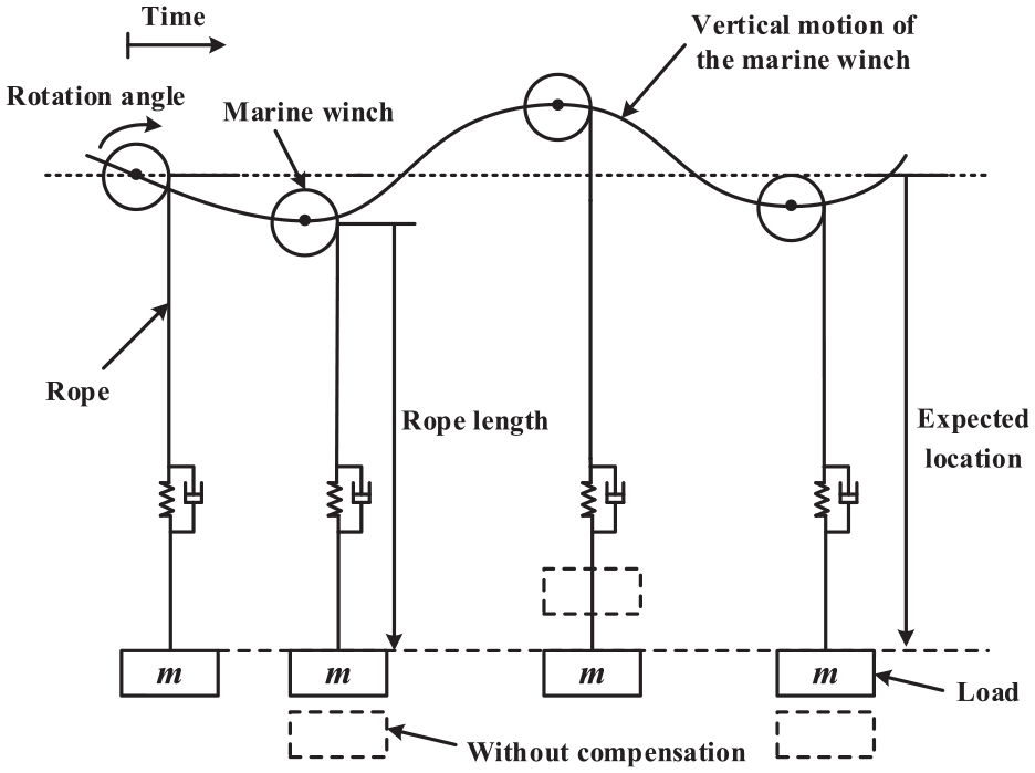
Schematic diagram of the heave compensation system.
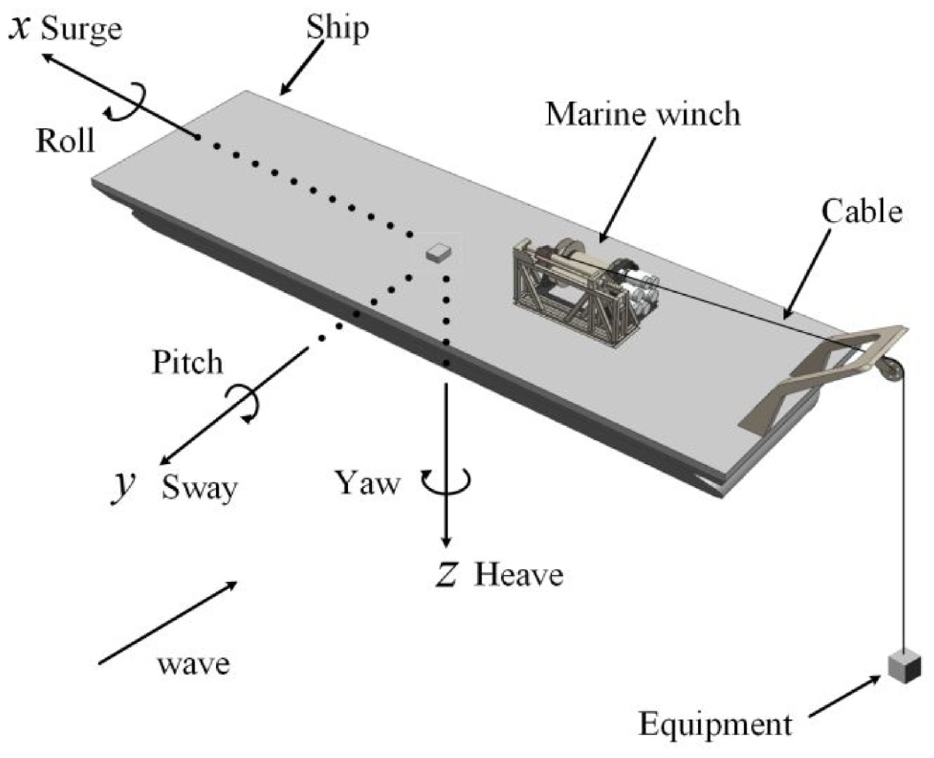
Composition of the AHC system.
Model of wave motion
The wave motion is a complex phenomenon in nature. The randomness of wind and the complex structure of wind field, along with other factors, make the wave motion present a strong randomness. Generally, the wave motion is the superposition of infinite cosine waves with different frequencies, amplitudes, initial phases, and propagation directions. Therefore, it can be expressed by formula (1). 22
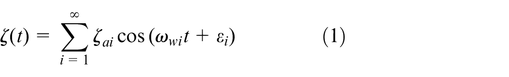
Where
From the spectral density of P-M spectrum, when the increment of angular frequency approaches 0, the amplitude of wavelet can be calculated by formula (2).
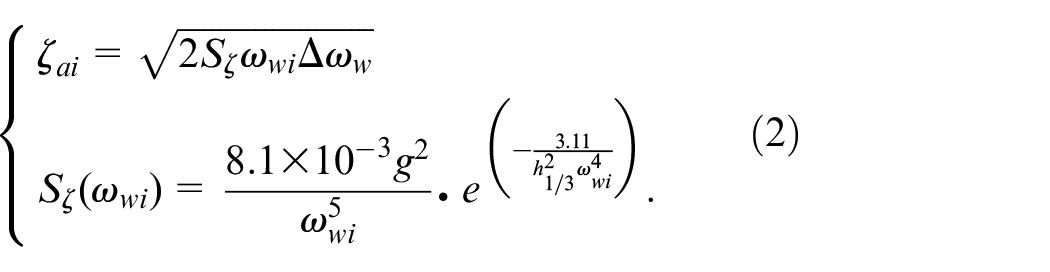
Where
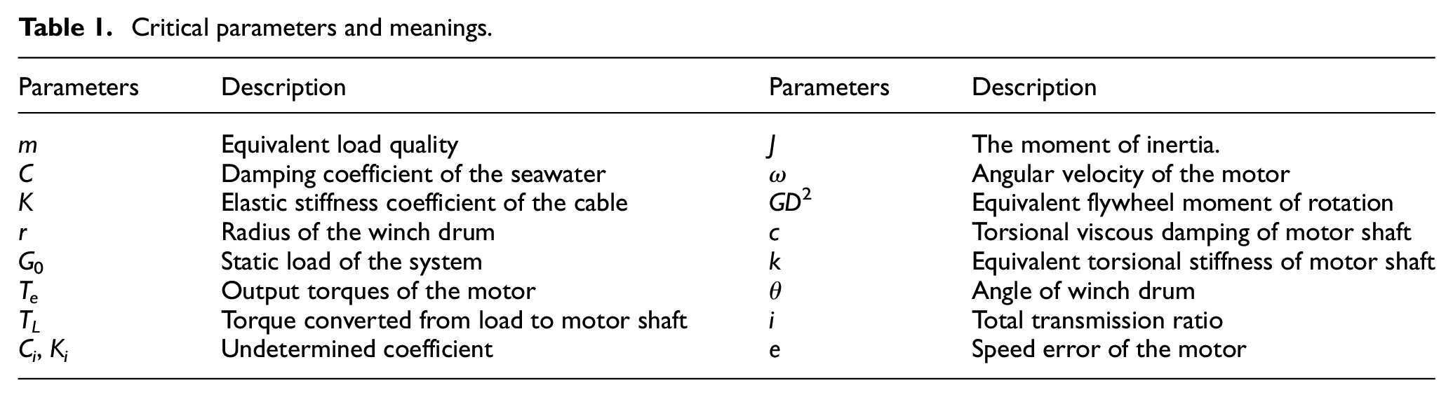
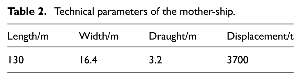
However, the empirical formula is not completely applicable to real sea conditions. Therefore, this work uses the heave displacement data collected by IMU under level 3 sea condition, so as to replace the empirical formula with the measured data. In this case, the effective wave height ranges from 0.5 to 1.25 m. Figures 3 and 4 show the spectrum and fitted curve respectively. The critical symbols and the meanings of the AHC system are shown in Table 1, the main technical parameters of the mother-ship are shown in Table 2.
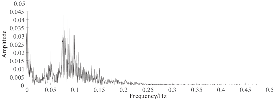
Spectrum of measured heave displacement. .
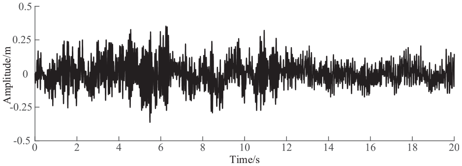
Fitted curve of measured heave displacement.
Critical parameters and meanings.
Technical parameters of the mother-ship.
Model of hoisting system
According to the reference, 23 the coupling system consists of equipment, cable, and seawater, which can be simplified as a mass-spring-damping system. The equation of motion can be expressed by equation (3).

Where
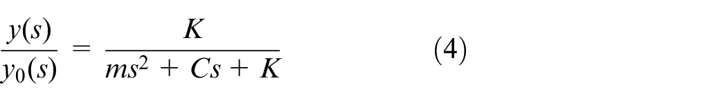
From equation (3), the transfer function of load displacement to ship displacement can be deduced as equation (4).
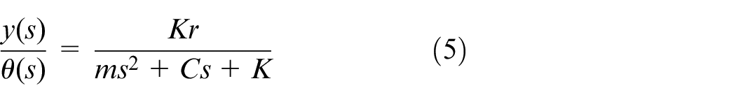
Moreover, the transfer function of load displacement to angle of winch drum can be described as equation (5).
Equation (6) is the computational equation of equivalent load quality.

Where
Meanwhile, the computational equation of damping coefficient of seawater can refer to equation (7).

Where
The elastic stiffness coefficient of the cable can be calculated by equation (8).
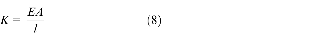
Where
Model of driving system
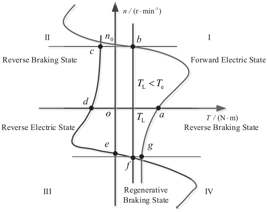
Figure 5 is the electromechanical characteristics of AHC motion. Apparently, the working quadrant of the motor is divided into four quadrants, while the three-phase asynchronous motor goes through five states. These are forward electric state (
Electromechanical process analysis of AHC motion.
When motor works in the first quadrant, the speed and torque of motor are positive, while the toque of load is negative. That is to say, the motor overcomes the torque of the load. When the speed of the motor approaches a higher value, the torque of the motor turns to be negative, and the redundant energy of the motor is consumed. This period, the process that power supply switches from forward direction to reverse direction has been completed. After that, the motor enters into the reverse braking state. It is notable that the above states of motor represent the process of hoisting load. When the speed of the motor reaches 0, the motor enters into the reverse electric state, and the speed increases inversely until it reaches to a higher value. Then, the motor enters into the regenerative braking state and the process that power supply switches from reverse direction to forward direction will happen. Finally, the motor enters into the reverse braking state and the speed of the motor decreases to 0 gradually. It is easy to find that the above states of the motor represent the process of lowering load. The analysis of this part is important to the model of AHC system, and the change of speed and torque should not be neglected.
The driving part of the marine winch is equipped with 6 three-phase asynchronous motors, while motors and winch drum are connected in meshing manner by pinions and annular gears. The simplified motion equation of the uniaxial electric driving system can be expressed by equation (9).
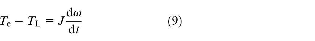
Where
Considering the transformational relationships like equation (10).
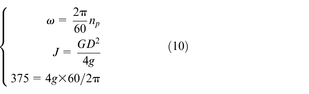
Where
Take the torsional viscous damping and equivalent torsional stiffness of motor shafts into consideration. Consequently, the operating equation of the driving system in the first quadrant can be expressed by equation (11).
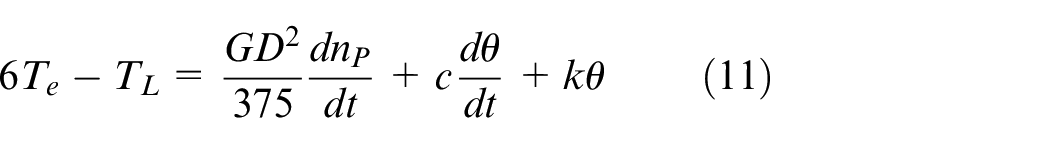
Where
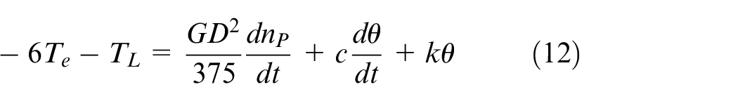
When the speed of motors approaches a higher value, the operating equation of the driving system at this period can be expressed by equation (12).
While the operating equations of driving system in the third quadrant and the fourth quadrant are expressed by equation (13) to (15) respectively.
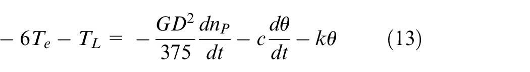
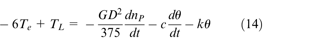
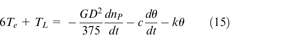
Furthermore, the torque converted from load to motor shafts can be expressed by equation (16), the total transmission ratio
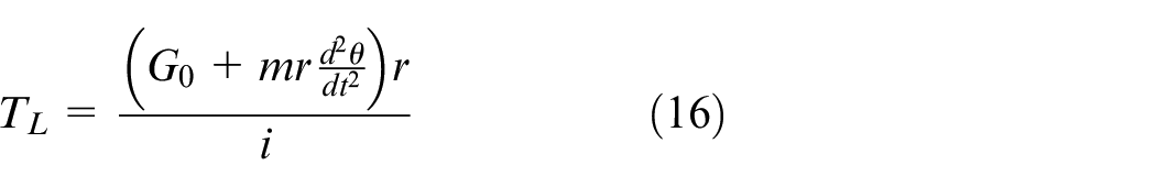
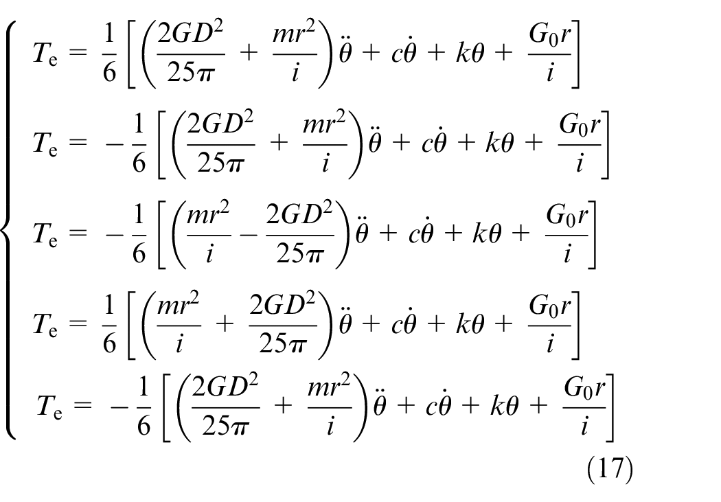
Substitute equation (16) into equations (11) to (15) separately, and the computational model of driving system at each stage can be obtained as equation (17).
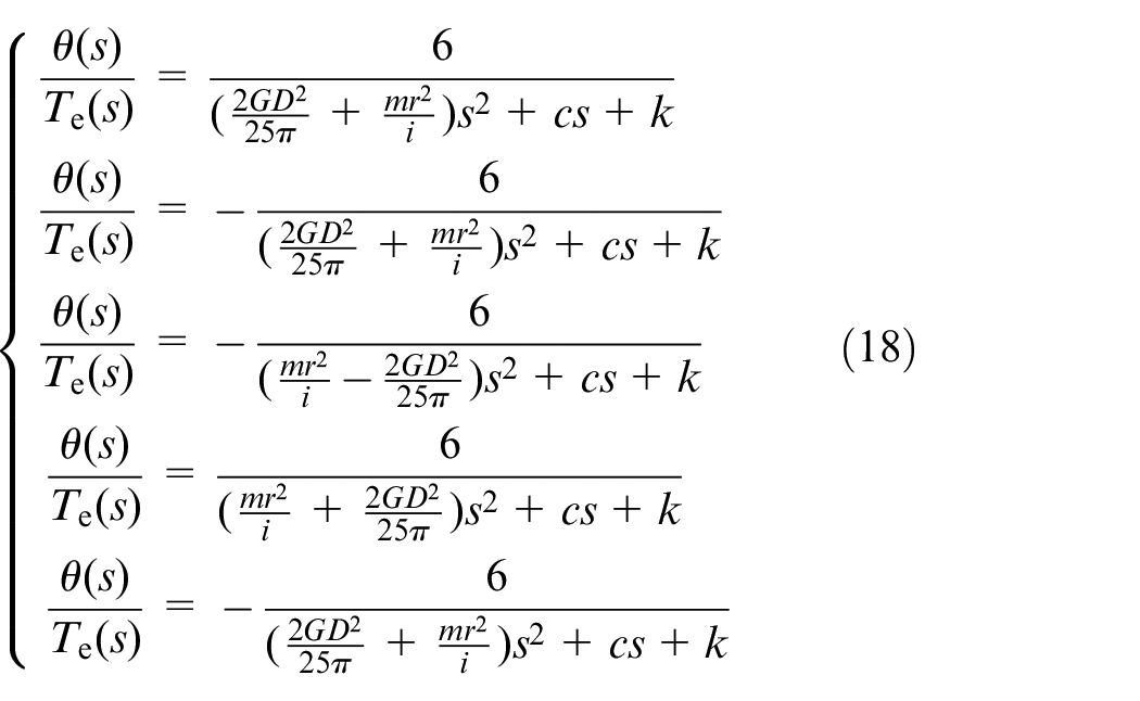
In combination with equation (5), the transfer functions of winch drum angle to motor torque can be obtained as equation (18).
Therefore, this work realizes the state equations related to the driving system by programming in Simulink.
Figure 6 is the control flow diagram of the driving system. Especially, the stability of the system in the flow diagram refers to transient stability, which indicates the system changes dynamically.
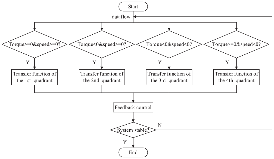
The control flow diagram of the driving system.
Model of control system for motors
The control system of the asynchronous motor has the characteristics of multivariable, strong coupling, and time-varying. To get better control characteristics of the asynchronous motor, it is necessary to realize the decoupling between stator currents. The most common used method is to combine vector control technology with the coordinate transformation theory. Thus, the voltage equation of the asynchronous motor can be described by equation (19).
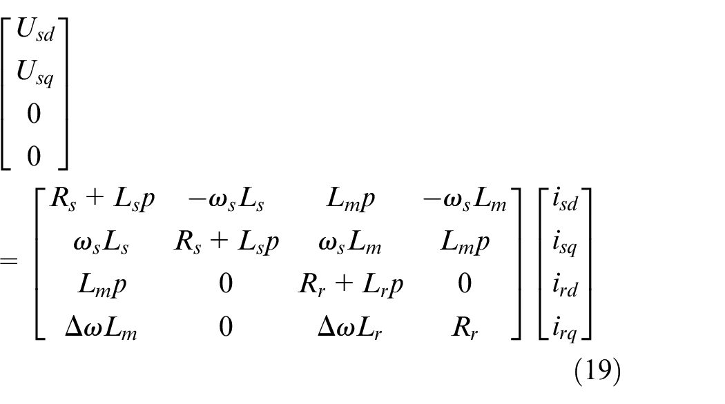
Where
Meanwhile, the equation of the asynchronous motor torque can be expressed by equation (20).
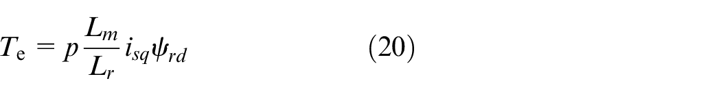
Where
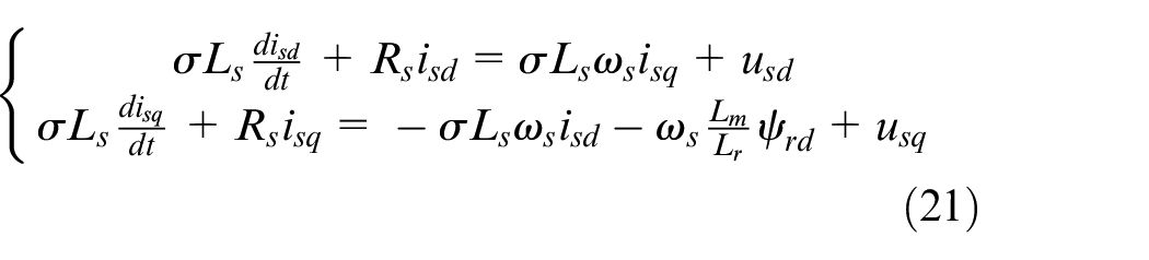
Where
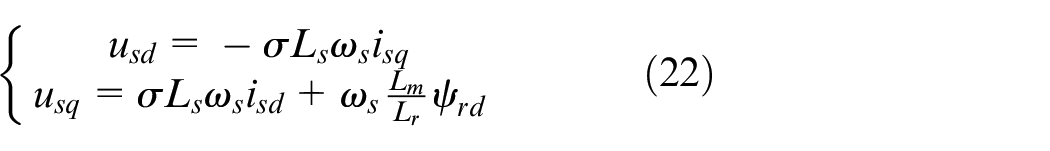
Equation (21) shows that there is coupling between d-axis stator current and q-axis stator current, it is necessary to design the decoupling circuit like equation (22).
The SMC has ideal switching characteristics with time-varying, which enables the system to move back and forth along the set sliding mode surface at a high frequency. Accordingly, it improves the sensitivity of the motor and loading capacity of the system, as well as the speed range of the system. Thus, this work attempts to replace the PI controller with the SMC in the speed regulator.
Figure 7 is the structure of SMC, the state variables of the controller are speed error

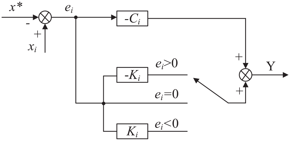
Structure of sliding mode controller.
Where
To satisfy the stability condition of the SMC and make the control approach to sliding mode surface as soon as possible, this work adopts the control rule shown in equation (24).

Where
To ensure the existence of sliding mode, equation (25) should be satisfied.

In general, the torsional viscous damping of the motor shafts and the equivalent torsional stiffness of motor shafts have little influence on the stability of the SMC. Therefore, considering the relationships in equations (9), (10) and (23), the rate of change
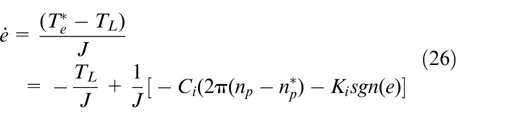
Substituting equations (23) and (26) into equation (25) yields equation (27).
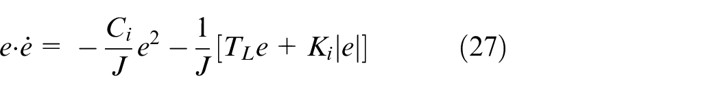
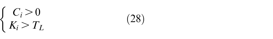
Equation (28) shows the condition for tenability of equation (27), which indicates there is a sliding mode surface in the design.
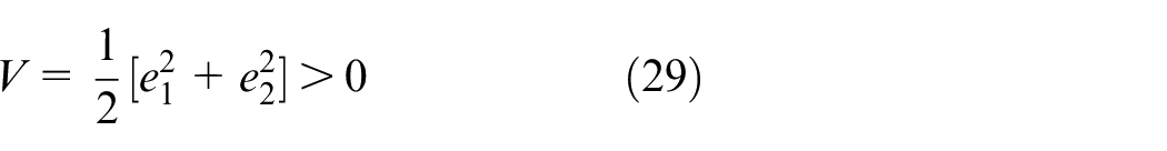
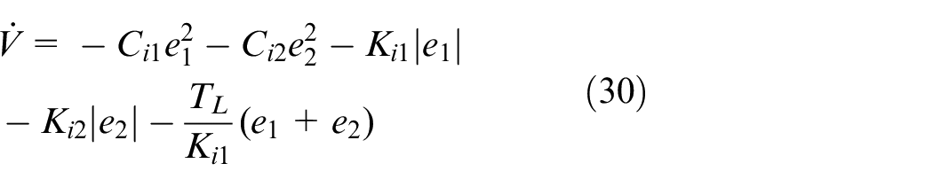
In addition, the Lyapunov function is defined in equation (29) to determine the stability of the SMC.
The derivation of equation (29) is expressed by equation (30).
To satisfy the condition
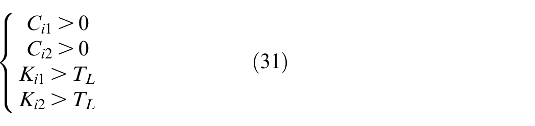
It can be inferred from equation (31) that the stability condition of the SMC is satisfied, which indicates the system is gradually stable.
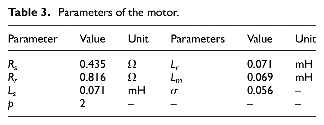
Figure 8 is a vector control system combined with SMC, the difference between the given rotor flux and the measured flux enters into the flux regulator (AFR), AFR outputs the d-axis stator current. Meanwhile, the SMC handles the speed error and outputs the given torque. The responsibility of the torque regulator (ATR) is to calculate the q-axis stator current. After calculation, the d-axis stator current and the q-axis stator current enter into the decoupling circuit, rotation transformation module, and space vector pulse width modulation (SVPWM) module, which means the signal processing has been completed once. Table 3 shows the parameters of the motor.
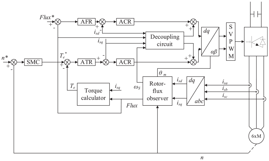
Diagram of the control system for motors.
Parameters of the motor.
Establishment of overall model
Figure 9 is the simulation model of AHC system for electric-driven marine winch, the name and function of each component are described as follows. The module marked “YY” is the input port of the measured heave displacement; the modules marked “torque-states-switch” and “angle-states-switch” are responsible for the conversion of working quadrants of the motor; the module marked “controlled motor” represents the speed control system of the motors; the module marked “Load Function” represents equation (4). The load displacement in offshore operation consists of the fixed position of load, the load displacement under the influence of excitation and the load displacement under the influence of AHC. The most critical index of the AHC system is compensated load displacement, which is the standard to evaluate the performance of the system. Generally, the smaller the compensated load displacement is, the better the effect of the AHC system is.
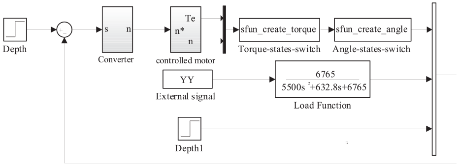
Simulation model of the AHC system.
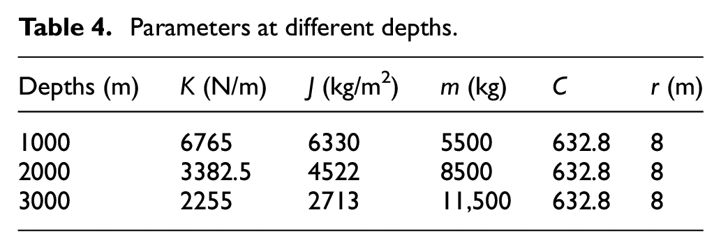
The simulation scheme assumes the load quality is 2.5 t, and the lengths of cable are 1000, 2000, and 3000 m respectively. Significantly, this work not only considers the capability of compensation, but also the change of the motor torque and the motor speed. The values of the related parameters under different conditions are shown in Table 4. We can infer from equations (4) and (5) that the length of the cable affects the transfer functions, and thereby affects the characteristics of the AHC system in varying degrees.
Parameters at different depths.
Results
The simulation results when the depth is 1000 m are shown in Figures 10 to 12. It can be seen from Figure 10 that the load displacement ranges from −0.2 m to +0.5 m. On the contrary, when the AHC function is enabled, the load displacement is greatly reduced, showing an ideal compensation performance of the system. Figures 11 and 12 are the curves of motor speed and motor torque respectively, both of them emphasize the working quadrants of the driving system. Especially, each quadrant is marked with a specific number which represents different working quadrants of the driving system. For example, at the beginning of the AHC function, the initial state of the system is lowering the load, that is the reason why the speed and torque are all negative. After that, the AHC system enters into the state of lifting the load, while the speed and torque turn to be positive. It is clear that the motor speed and motor torque in each quadrant are in accordance to what they are expected. In detail, the motor speed ranges from −700 to +300 rpm, and delta torque of the motor fluctuates between −100 and +60 Nm.
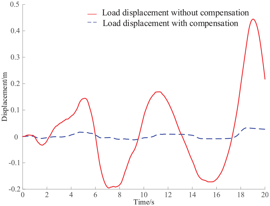
Result of load displacement when depth is 1000 m.
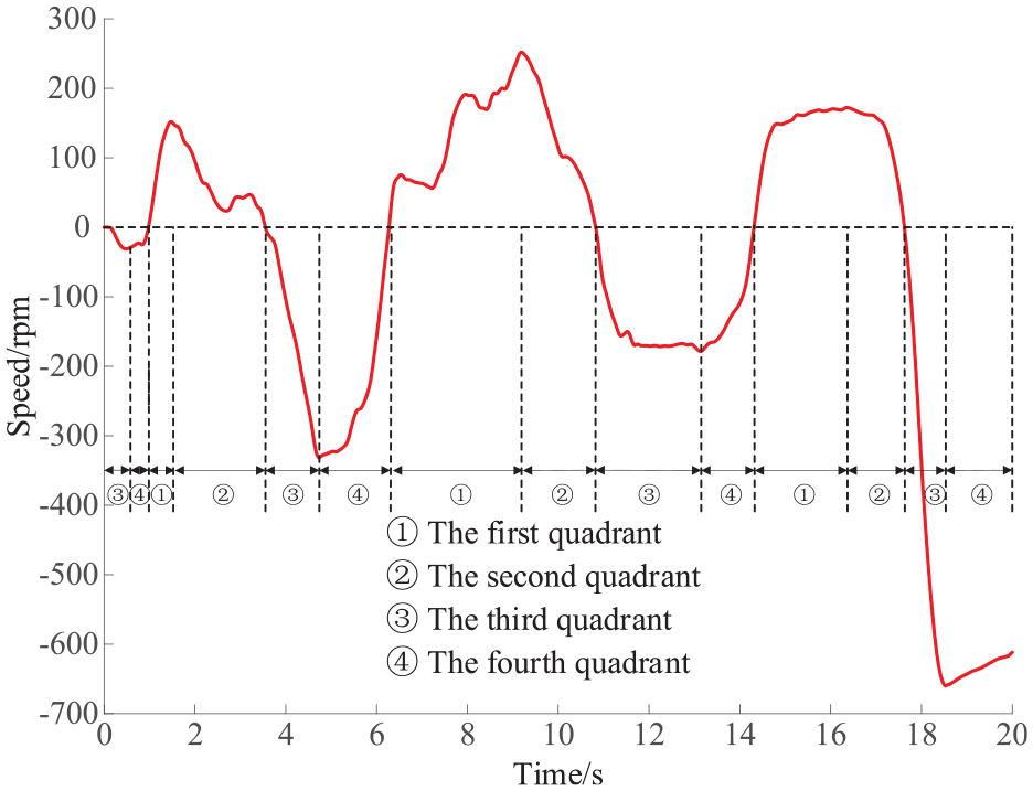
Result of motor speed when depth is 1000 m.
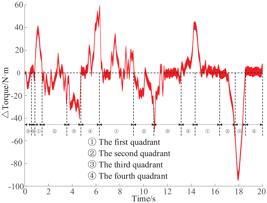
Result of motor torque when depth is 1000 m.
Contrary to the earlier simulation, the following scheme adopts the parameters when depth is 2000 m. In addition, the simulation considers the situation that motors only work in general conditions. From Figure 13, the load displacement without compensation ranges from −0.8 m to +0.8 m, while the load displacement with compensation is reduced exponentially. Compared with the previous simulation results, Figures 14 and 15 reflect some delicate changes. For example, the curves without considering working quadrants of the driving system are also demonstrated in the diagrams at the same time. By comparing the simulation results under different considerations, it can be founded that the results of the latter show no regularity in distribution of speed and torque, which reveals the irrationality of system modeling. Similarly, the motor speed ranges from −600 to +600 rpm, and the delta torque of the motor fluctuates between −160 and +80 Nm.
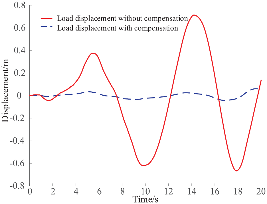
Result of load displacement when depth is 2000 m.
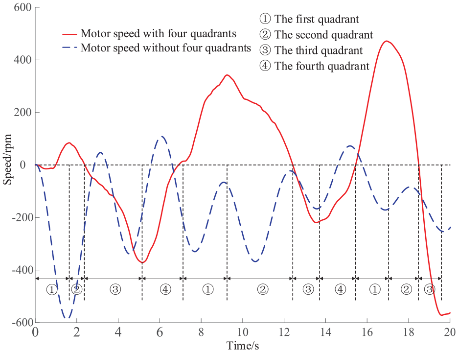
Result of motor speed when depth is 2000 m.
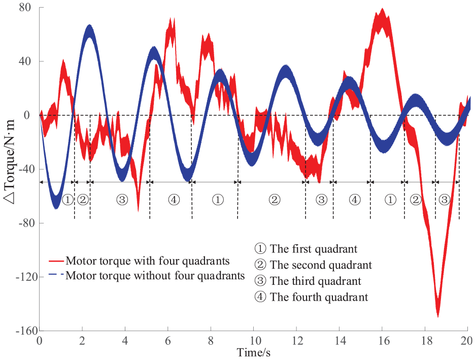
Result of motor torque when depth is 2000 m.
The last simulation scheme adopts the parameters when depth is 3000. From Figure 16, the load displacement without compensation ranges from −2.0 to +2.0 m, and the load displacement is also reduced significantly after compensation. From Figures 17 and 18, the motor speed ranges from −800 to +1000 rpm, while the delta torque of the motor fluctuates between −170 and +130 Nm. Furthermore, from the results of the motor speed and the motor torque, the same conclusions can be obtained just like those of previous simulations.
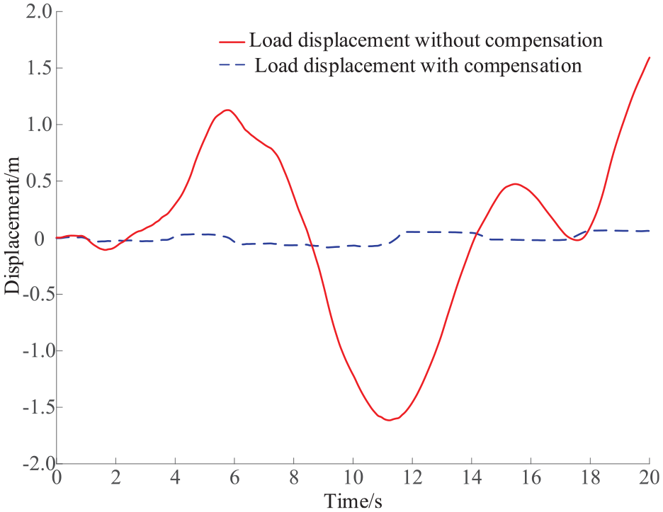
Result of load displacement when depth is 3000 m.
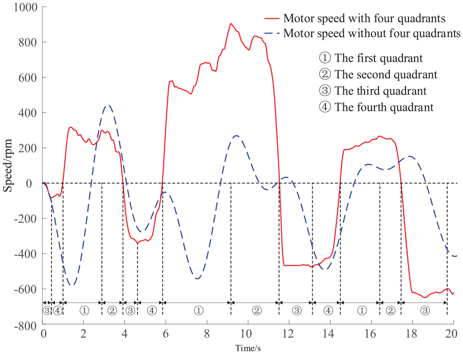
Result of motor speed when depth is 3000 m.
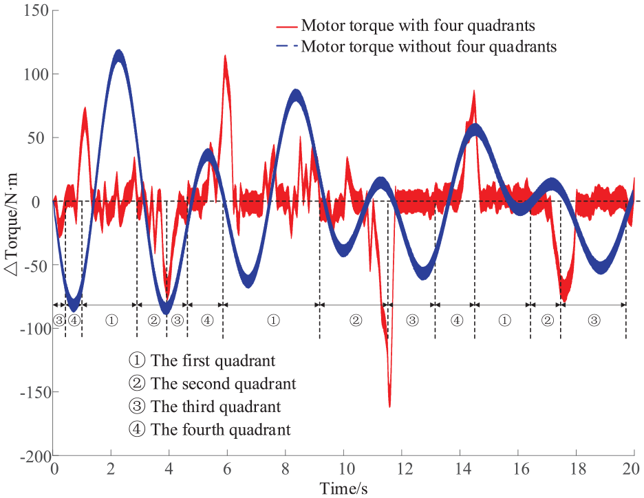
Result of motor torque when depth is 3000 m.
From the ordinate systems in different figures, the compensation performance at different depths is proved to be ideal. The absolute values of different compensated load displacements are used to evaluate the performance of the system. The absolute value in the first simulation is smaller than 0.05 m, the second simulation is smaller than 0.1 m, while the last simulation is smaller than 0.2 m.
By comparing simulation results under different assumptions, some potential patterns can be exploited. For instance, with the increase of the depth, the variation range of the load displacement becomes larger. Meanwhile, similar information can be obtained from the curves of the motor speed and the motor torque. That is, the larger the depth is, the larger the variation range of the motor speed is, as well as the motor toque. It can be inferred that depth is one of the factors which is related to the effect of the AHC system. Moreover, from the phenomenon that the variation range of the motor torque increases, the conclusion that deep-water operation is more complex and dangerous than offshore operation can be obtained, verifying that deep-water operation causes the cable to be broken more easily.
In offshore operation, the compensation capacity of the AHC system is required to be
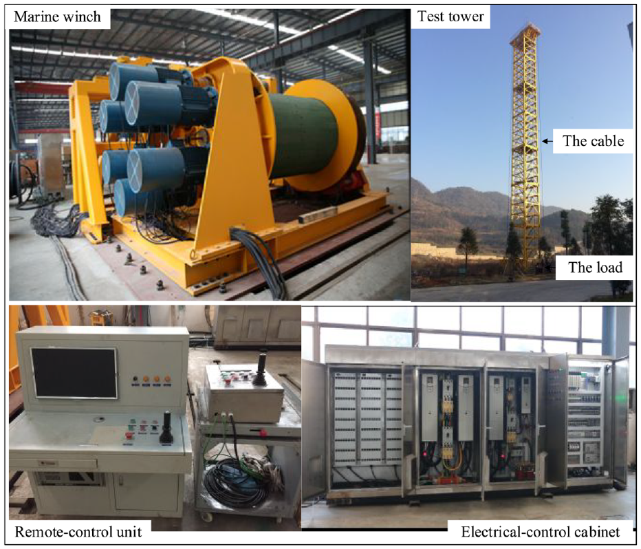
Experimental platform.
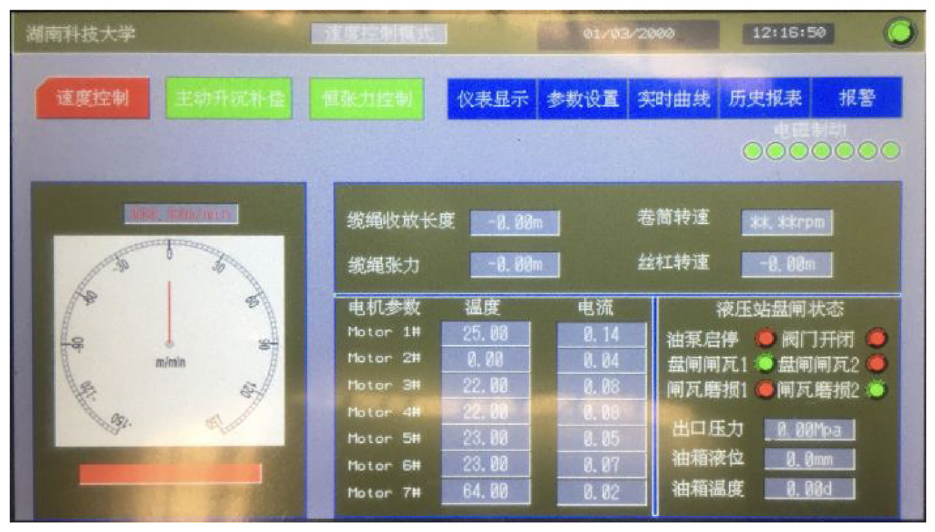
Diagram of the computer monitoring interface.
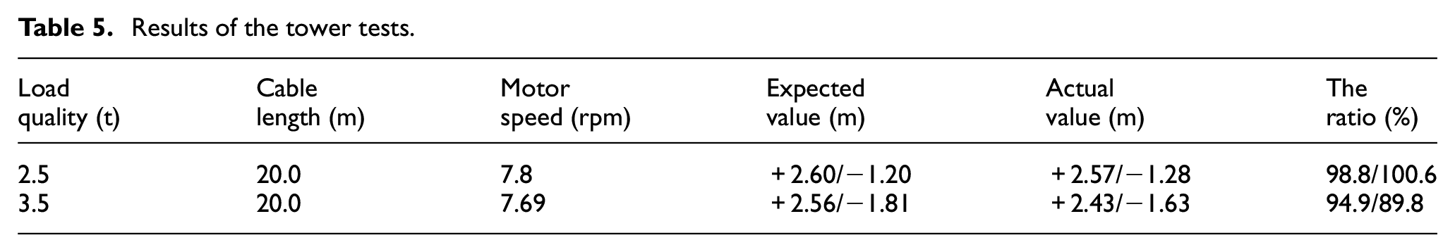
The detailed scheme supposes the marine winch is fixed, and the equivalent quality of the load is replaced by adopting the method of counterweight. The test results, which adopt the average value of repeated tests, are shown in the form of historical reports. Eventually, the reports are shown in the form of curves. Typically, to verify the correctness of system modeling, the results when equivalent qualities of the load are 2.5 and 3.5 t will be introduced, and the experimental data are displayed in the form of tabular data to give an intuitive representation (Table 5).
Results of the tower tests.
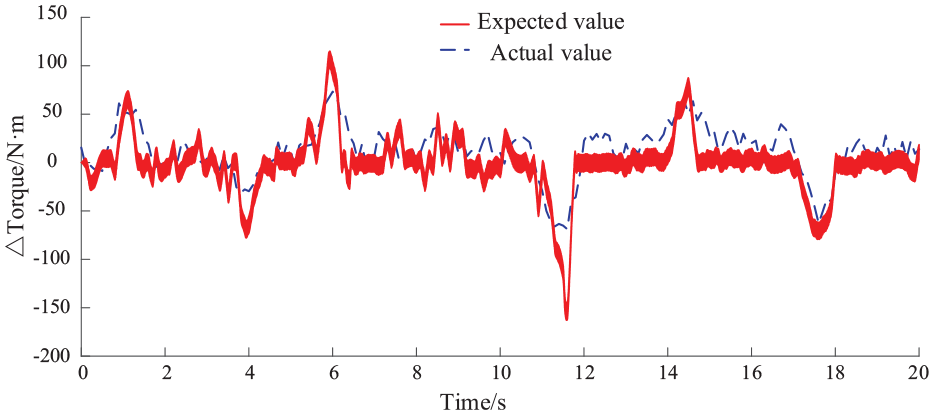
The experimental results of the load displacement and the motor torque are shown in Figures 21 to 23. Obviously, the experimental load displacement is greatly reduced after compensation, which means the decoupling of wave motion and load motion is realized. Meanwhile, it can be founded that the experimental torque result is essentially consistent with that of simulation, which proves the validity of system modeling.
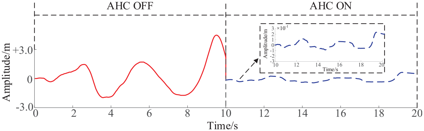
Result of the experimental displacement.
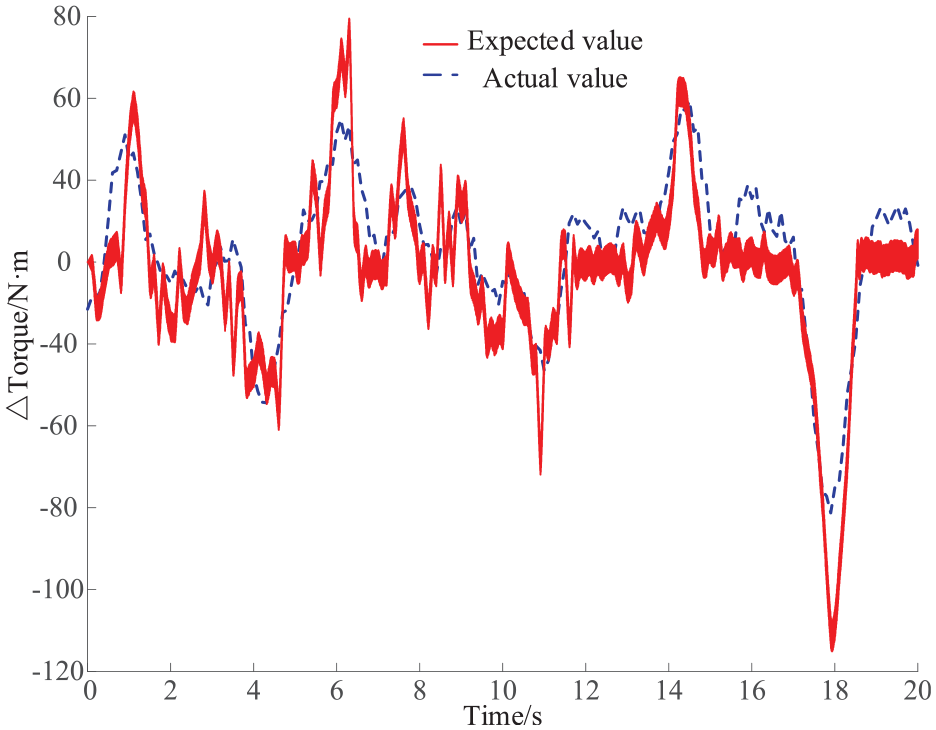
Result of the experimental torque when depth is 1000 m.
Result of the experimental torque when depth is 3000 m.
Conclusion
This article has presented an AHC approach for electric-driven marine winch proposing a working quadrant concept. The work replaces other forms of heave compensation system with the electric-driven AHC system, as well as the wave excitation. The working concept is involved in the operation of a multi-motors driving system. Accordingly, the equations that the driving system works in each quadrant are derived. In addition, the simulation only considers general condition is implemented as comparison. The compensation algorithm based on the principle of sliding-mode control algorithm is adopted to overcome the problem caused by switching of working quadrant, such as chattering effect and system delay.
Active heave compensation test tower is used to evaluate the overall compensation performance of the system, as well as system modeling. The results of the compensated load displacement show a high precision of the AHC function, the average compensation rate of the system reaches as high as 96.03%. Also, the response time of the system is proved to be pretty good. The results of the motor speed and the motor torque show both of them are in accordance to what they are expected in each quadrant, which proves the theoretical analysis is correct. Referring to the overall compensation performance, the proposed AHC approach is proved to be effective. Hence, this method is intended to be widely used in new types of AHC system in the future.
Footnotes
Declaration of conflicting interests
The author(s) declared no potential conflicts of interest with respect to the research, authorship, and/or publication of this article.
Funding
The author(s) disclosed receipt of the following financial support for the research, authorship, and/or publication of this article: The authors gratefully expressed their thanks for the financial supported by the National Natural Science Foundation of China (Grant No. 52075163).