Sage Journals: Discover world-class research

Abstract

To enhance the joint control performance in hydraulic quadruped robots, active disturbance rejection control was used in the leg joint controller design of a hydraulic quadruped robot in combination with the self-growing lévy-flight salp swarm algorithm in this paper. First, the robot-leg structure of the hydraulic system model was built to analyze system operation details in terms of the mathematical construction. Second, the self-growing lévy-flight salp swarm algorithm was introduced. Then, the active disturbance rejection control parameters required were defined based on the composition and principle of the third-order active disturbance rejection control model. Third, the system evaluation function ITSE was selected, and the parameter tuning problem was converted into an algorithm optimization problem. Finally, the joint system of the hydraulic quadruped robot was taken as the research object, the self-growing lévy-flight salp swarm algorithm was added to the active disturbance rejection control to tune parameters, and this paper compared three different algorithms in the same environments to show the good control ability of the proposed method. To comprehensively show the performances of robot joint systems controlled by the proposed controller, the temporal response results, the frequency response results, the sawtooth response results, the ramp response, and the random response were displayed. All results reveal the effectiveness and excellent performance of the proposed controller in joint systems of a hydraulic quadruped robot.

Keywords

Salp swarm algorithm hydraulic quadruped robot active disturbance rejection control

Introduction

Hydraulic quadruped robots are commonly used in many fields because of their unique advantages, including their ability to overcome obstacles, execute wild tasks, and adapt to unknown environments.^1,2 During robotic running and jumping, the joints frequently interact. The output signals of other joints affect the input of one joint, and at the same time, the output of one joint affects the input signals of other joints.^3,4 Therefore, there is a coupling phenomenon among robot joints. This phenomenon introduces many difficulties to the control method of robot joint control; thus, determining the strategies among robot joints has become one of the most difficult problems. Hydraulic robot joints are mainly driven by hydraulic systems. For a hydraulic robot, different highly integrated valve-controlled cylinder systems comprise the robot driving component.^5,6 The hydraulic drive system includes not only high control accuracy but also dynamic compliance performances. Thus, the impact on robot joints can be weakened, which can protect the robot components and enhance robot moving stability.⁷

Hydraulic systems have not only good power-to-weight ratios but also strong loading capacities and high response speeds, which makes hydraulic systems appropriate for robot joint driving systems.^8–10 Therefore, the valve-controlled hydraulic system is the most common joint control actuator in hydraulic quadruped robots. When hydraulic quadruped robots are running, feedback loading exists between the different joints. Therefore, there is a need for control precision and shock absorption in hydraulic systems, which can protect robot components. Due to the mechanical size, external loading, and creeping at low velocity, hydraulic systems require synchronization and precise control strategies. Hydraulic quadruped robots usually work in different environments, such as in mountains, jungles, snow areas, and forests. Therefore, it is important to meet the control requirements of robustness, flexibility, lower construction cost, precision, dynamic compliance, and applications in different systems.^11–17 There are many advanced control methods at present.¹⁸ But there will be a large contact force when the robot foot contacts with the ground in robot joint systems. It will produce a very large impact force in robot joints when the foot collides with the ground. In order to avoid excessive contact force and ensure the moving flexibility in the contact process when the robot contacts the ground, anti-disturbance control should be added to the robot control system. At present, traditional anti-disturbance control methods mostly use passive compliant devices, simple compliant control algorithms, and improving position control performances to get a satisfactory anti-disturbance performance. Some traditional anti-disturbance control methods can not meet requirements of the leg joint control in the hydraulic quadruped robot. So this paper selected the active disturbance rejection control algorithm in the leg joint control of the hydraulic quadruped robot to get a better anti-disturbance control performance. The ADRC control effect mainly depends on whether its parameters are adjusted properly.

Active disturbance rejection control (ADRC), which is a useful observer mixed with disturbance attenuation control, was proposed by Han et al.¹⁹ to provide an alternative control approach to PID and has become an attractive control method. External-internal disturbances and unmodeled dynamics can be seen as the generalized disturbance, which is treated as the extended state in ADRC. Then, ADRC applies a nonlinear extended state observer to estimate and compensate for the nonlinear error, and the total disturbances in the systems can be viewed not only as an additional state variable but also as matched signals with bounded or constant derivatives. The ESO estimates both the states of disturbances and feed-forward compensation.^20–24 ADRC cannot achieve a perfect performance and the controlled systems have poor response characteristics if reasonable ADRC parameters cannot be found. The optimal ADRC parameters can be used in robot joints to maximize the jumping and running abilities of robots. Therefore, it is crucial to obtain the best ADRC parameters in industrial fields.

Traditional ADRC parameter tuning methods mainly include the experience and trial-and-error method, the parameter tuning method based on the time scale, the dynamic parameter tuning method, and the optimization fitting setting method. The common experience and trial-and-error-method highly depend on the designer’s experiences, and the setting procedure is complicated, time-consuming, and limit.¹⁹ In the engineering practice, the parameter tuning method must analyze factors including the signal bandwidth, different noises, disturbances, and sampling steps. Therefore, the parameters obtained by designers experiences are still limited in practical application. The parameter tuning method based on time scale²⁵ can determine the controller parameters. However, due to the calculation complexities of the time scale and limitations of the sampling time, the practical application of the method is limited. The dynamic parameter tuning method²⁶ is that TD, ESO, and NLSEF can be seen as the independent individuality. Parameters of TD and ESO are tuned to achieve satisfaction, then, other parameters of ADRC can be adjusted by combining with NLSEF. This method offers the general rule of the ADRC parameter tuning method, but it still belongs to the experience method due to clear guidance lacking. The optimization fitting setting method²⁷ owns advantages of the experience and trial-and-error method, and comprehensively considers the factors including sampling steps and noises. However, the method is more complex, and the application is not obvious for large range parameter tuning in ADRC. The artificial intelligence method is easy to practice, can less consider bandwidths, noises, and sampling steps only needs to define the corresponding searching range and the objective function. The ADRC parameter tuning problem is transformed into the optimization problem in the artificial intelligence method. Firstly, the ADRC parameters will be applied to the system to get the objective function value. Then, the function value of each iteration will be used as the initial value of the next iteration. Finally, the artificial intelligence method will converge to the result after the iteration process. With the development of the research on artificial intelligence, meta-heuristic algorithms applied in ADRC tuning methods have became more and more popular in recent years. Zhang et al.²⁸ designed ADRC via levy flight-based pigeon-inspired optimization for small unmanned helicopters. Kang et al.²⁹ used a hybrid algorithm based on the fish swarm algorithm and the particle swarm optimization algorithm to tune ADRC for the flight attitude control of the unmanned aerial vehicle. Cai et al.³⁰ proposed a new active disturbance rejection control based on the chaotic gray wolf optimization in the quadrotors to achieve trajectory tracking and obstacle avoidance. Literature³¹ used the adaptive particle swarm optimization algorithm (APSO) to find the feasible ADRC parameters to meet the performances of the induction motor and the disturbance compensation. Wang et al.³² created the disturbance rejection controller based on an artificial bee colony algorithm for the train traction system. Hai et al.³³ drafted an enhanced ADRC for the robot attitude deformation system in conjunction with an evolutionary game theory-based pigeon-inspired optimization. Wei et al.³⁴ used the ameliorated shark smell optimization algorithm for tuning ADRC parameters in two degrees of freedom manipulator.

The salp swarm algorithm (SSA), inspired by salp swarm behaviors, was proposed by Mirjalili et al.³⁵ Salps form swarms called salp chains in the deep ocean; these chains can achieve better locomotion during the foraging procedure. A salp chain can be divided into two parts to formulate the mathematical model: one leader and several followers. The leader position is at the beginning of the salp chain, while the rest of the chain is regarded as the followers. Salps update their positions by relying on the positions of their neighbors. Each salp in the salp chain can be seen as a feasible solution to the search problem, and each function value corresponding to an individual position is its fitness. To enhance the search accuracy and the convergence rate, some SSA variants have been given in the literature and used in many industrial fields, such as Refs.^36–42 One such variant is the self-growing lévy-flight salp swarm algorithm (SG-LSSA), which has been used in hydraulic systems to find three PID parameters. The SG-LSSA uses the large initial leader step and the self-growing updating strategy to boost the search speed of the basic SSA and uses the lévy-flight method to heighten the algorithmic diversities. In this paper, the ADRC parameter tuning problem was taken as the research background. The influence of the ADRC parameters on the robot joints and the optimization performances of the SG-LSSA were analyzed. Thus, the ADRC parameter tuning problem was solved by the SG-LSSA for a hydraulic quadruped robot.

According to the uncertain disturbance in the hydraulic quadruped robot, a third-order active disturbance rejection control strategy is proposed in the joint control system of the hydraulic quadruped robot. Aiming at the problem that it is difficult to select the feasible ADRC parameters, a parameter selection strategy based on SG-LSSA is added in the third-order ADRC controller. The proposed SG-LSSA-ADRC controller can effectively suppress disturbances in different environments when the robot contacts the ground. In this paper, ADRC is applied to the joint control system of the hydraulic quadruped robot to solve the problem caused by a series of disturbance factors in the control system. However, ADRC has many parameters. If the reasonable control parameters cannot be selected, the controlled system will not achieve the desired performance, which will have adverse effects in the robot moving. To control the robot effectively and enhance the jumping and running abilities, this paper selected the SG-LSSA algorithm to find the reasonable ADRC parameters, and used SG-LSSA-ADRC in the joint force control system of hydraulic quadruped robot to boost the robustness, the stability, and the anti-interference characteristic in the hydraulic quadruped robot.

Three major contributions in this paper are summarized as follows:

This paper built the three-order ADRC controller by controlled system models and gave 16 ADRC parameters in the leg joint control of a hydraulic quadruped robot.

ADRC parameters searching problem was converted into the 16 dimension optimization problem, and this paper used SG-LSSA to find reasonable ADRC parameters in a hydraulic quadruped robot.

For the leg joint control of a hydraulic quadruped robot, an SG-LSSA-ADRC controller was designed to improve system performance. Then, this paper used the step signal, the sinusoidal signal, and the sawtooth signal, the ramp signal, and the random signal to show different performances of the proposed ADRC controller in a hydraulic quadruped robot.

In this paper, Section “The hydraulic quadruped robot system” introduced the robot mechanical structure and the hydraulic system’s physical model. Section “Self-growing lévy-flight salp swarm algorithm” introduced SG-LSSA. Sections “Active disturbance rejection control” and “The proposed control method” introduced the ADRC model and the proposed controller. Section “Discussion” showed all result analyses of step signals, sinusoidal signals, and sawtooth signals.

The hydraulic quadruped robot system

The hydraulic quadruped robot system mainly includes a frame and a four-leg structure. Each leg has a rolling hip joint, pitching hip joint, and pitching knee joint. The power driving system consists of a hydraulic oil tank, a constant-pressure variable pump, a single-cylinder gasoline engine, an electrohydraulic servo actuator, and other hydraulic accessories. Each active degree of freedom is driven by the same hydraulic systems. The electrohydraulic servo actuator integrates an asymmetrical flow servo valve, an asymmetric hydraulic cylinder, and a displacement sensor. The passive degree of freedom is composed of a linear bearing and a damping spring, which is mainly used to absorb the impact force of the foot to protect the robot. The single-leg structure of the hydraulic quadruped robot is shown in Figure 1.

Figure 1.

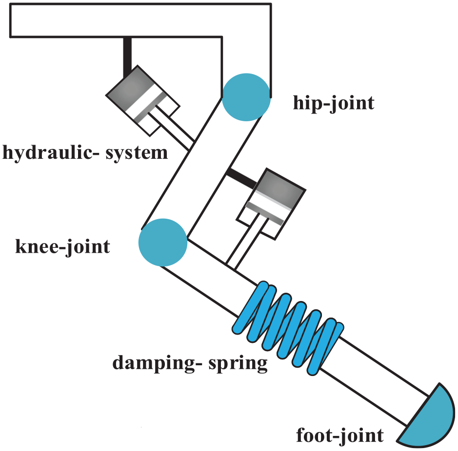
The single-leg structure.

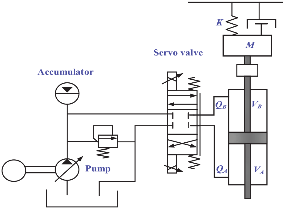
Figure 1 is the single-leg structure including, two hydraulic-systems, one hip-joint, one knee-joint, one damping-spring, and one foot-joint. Two hydraulic systems can drive the robot leg work because the hydraulic system can give stable performance and can work in different loading environments, so two hydraulic systems are significant. And hydraulic systems can be used to realize the hip joint yaw motion and the pitch motion of the hydraulic quadruped robot. To show the hydraulic system structure principle, this paper gives the hydraulic system structure in Figure 2 and the transfer function model of the hydraulic servo system. If the hydraulic model is known, the hydraulic model can be used in the simulation experiment before the practical experiment. In the real industry, many industry experiments cannot be carried out many times due to the limitation of materials and the bad situation of the experimental environment. The hydraulic system model can help to quickly measure the effectiveness of the proposed method before the actual industry testing, which greatly reduces the measurement time and industry wasting. In the hydraulic quadruped robot, hydraulic systems are used to realize the joint swing-pitching. The basic working model of the hydraulic system is shown in Figure 2, the system model mainly involves the servo valve and the hydraulic cylinder, and the hydraulic cylinder is drove by the three-landing-four-way servo valve. In Figure 2, Q and Q_AB are the flow of two chambers, M (kg) is the total mass of piston and loading referred to the piston, K (N/m) in the spring gradient, A (m²) is the effective area of the piston, B_p (N/(m/s)) is the viscous damping coefficient, V_A (m³) and V_B (m³) are two volumes of two chambers. The voltage signal will be transformed as the current signal in the servo amplifier. Then, the current signal will control the slide valve and the flow rate. Finally, hydraulic systems are controlled by signals which are fed back by the A/D system. The internal-external leakage is the laminar flow. The flow at the orifice is turbulent flow the oil temperature and the volume elastic modulus are constant. There are two states in the normal hydraulic system, which call the dynamic state and the steady-state. When input signals are not changed in the control system, the whole system finally reaches the equilibrium state, which calls the steady-state. When the controlled system in the steady-state receives disturbances, output signals will change until the next steady state is established. The dynamic characteristic refers to the system response process from the initial state to the final state under typical signals, and the system dynamic characteristic can be expressed by differential equations. The pressure is the force on a unit area perpendicular. The flow refers to the amount of the fluid flowing through the effective section of the closed pipe or the open channel in the unit time. The pressure depends on the external load, and the flow rate determines the speed. The flow characteristic refers to the relationship between the flow coefficient and the intercepting element stroke when the pressure drop through the valve is constant and the intercepting element moves from the closed position to the rated stroke. The flow equation of the hydraulic control valve, the flow continuity equation of the hydraulic cylinder, and the hydraulic cylinder – loading force balance equation were calculated to build the transfer function of hydraulic power components.

Figure 2.

The basic working model of the hydraulic system.

The valve is a zero-opening four-sided spool valve, which has matched and symmetric four throttle-openings are matched and symmetric, the giving oil pressure is constant, and the return oil pressure is zero, the flow equation of the hydraulic control valve can be built as

Q_{L} = K_{q} X_{V} - K_{c} P_{L}

(1)

where P_L (Pa) is the pressure drop between the two chambers, P_L = P_A − P_B, P_A (Pa) and P_B (Pa) are the rodless cavity loading and the rod cavity loading, X_V is the spool displacement, K_q and K_c are the flow gain and flow pressure coefficient. K_q and K_c can be written as

K_{q} = C_{d} w \sqrt{\frac{(P_{s} - sgn (X_{V}) P_{L})}{ρ}}

(2)

K_{c} = C_{d} w | X_{V} | \sqrt{\frac{1}{4 ρ (P_{s} - sgn (X_{V}) P_{L})}}

(3)

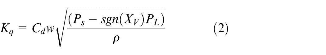
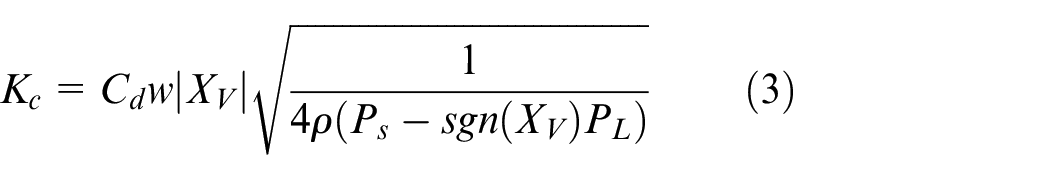
where C_d (m³/(s.Pa)) means the discharge coefficient, and w (m) is the constant area gradient, ρ (kg/m³) is the oil mass density, P_s (Pa) is the hydraulic supply pressure, sgn means the signum function. Inlet-outlet oil flow Q_A and Q_B in the hydraulic cylinder can be expressed as

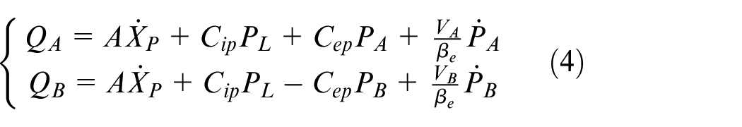
{\begin{matrix} Q_{A} = A {\overset{\cdot}{X}}_{P} + C_{ip} P_{L} + C_{ep} P_{A} + \frac{V_{A}}{β_{e}} {\overset{\cdot}{P}}_{A} \\ Q_{B} = A {\overset{\cdot}{X}}_{P} + C_{ip} P_{L} - C_{ep} P_{B} + \frac{V_{B}}{β_{e}} {\overset{\cdot}{P}}_{B} \end{matrix}

(4)

where C_ip (m³/(s.Pa)is the represent the internal leakage coefficient, C_ep (m³/(s.Pa) is the external leakage coefficient, β_e (N/(m².Pa)) is the oil effective bulk modulus.

The liquid compression influencing is the biggest, and the damping ratio and the natural frequency both are smallest when the piston is in the middle position. Therefore, the middle position of the piston should be taken as the initial position, Q_L = (Q_A + Q_B)/2. So, the flow continuity equation of the hydraulic cylinder.

Q_{L} = A {\overset{\cdot}{X}}_{P} + (C_{ip} + \frac{C_{ep}}{2}) P_{L} + \frac{V}{4 β_{e}} {\overset{\cdot}{P}}_{L}

(5)

The hydraulic component dynamic characteristic is influenced by loading characteristics, and the loading mainly includes viscous damping, the inertial force, and some external arbitrary loading, and the hydraulic cylinder-loading force balance equation can be calculated as

M {\overset{\cdot\cdot}{X}}_{P} = A P_{L} - B_{P} {\overset{\cdot}{X}}_{P} - K X_{P} - F_{g}

(6)

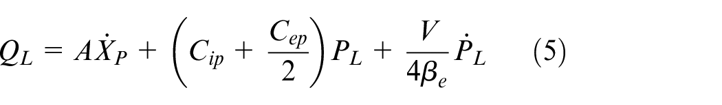
where X_P is the piston displacement. Figure 3 is the hydraulic cylinder displacement block diagram obtained from the loading flow. This paper can get the hydraulic cylinder displacement block diagram obtained from equations (1) to (6), which was shown in Figure 3.

Figure 3.

The hydraulic cylinder block diagram.

Self-growing lévy-flight salp swarm algorithm

SSA is a new metaheuristic algorithm which mimics the salp swarming behaviors. Salps own barrel-shaped bodies and move around as chains. In SSA, moving behavior is a mathematical model to solve optimization problems. There are two main types of salps including one leader salp and followers in SSA. The leader in the front direction leads the salp swarming chain, and all followers follow the leader to find the food source. The self-growing lévy-flight salp swarm algorithm (SG-LSSA) used the self-growing strategy and the lévy-flight mechanism in basic SSA to boost the searching diversity and performance of SSA. The self-growing strategy can weaken the high randomness of the lévy-flight mechanism, which is proposed in 1952 by French mathematician lévy.

With time continuing, the leader position adjustment can get more and more subtle, and the searching scope is gradually changed from large to small. The SG-LSSA process can be described as follows:

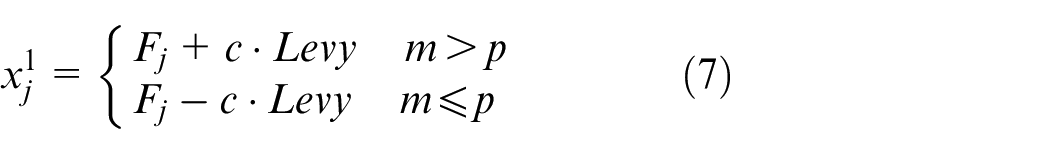
Step 1. Initialization. Initially set the D-dimensional finding scope, set the maximum number of search iterations T, generate N salps positions $x_{j}^{i}$ , j is the dimension of the searching space, i is the ith salps position, define the searching scope [lb_j ub_j], set the current iteration t equals to 1. Set probability factor p.

Step 2. Update the leader position. The movement of the leader position can be modeled as:

x_{j}^{1} = {\begin{matrix} F_{j} + c \cdot Levy \begin{matrix} m > p \end{matrix} \\ F_{j} - c \cdot Levy \begin{matrix} m \leq p \end{matrix} \end{matrix}

(7)

where $x_{j}^{1}$ is the leader salp position, F_j means the food source position, p is a probability coefficient in the interval of [0, 1], m is the random number in the interval of [0, 1]. The coefficient c can be described as:

c = (u b_{j} - l b_{j}) (1 - t / (T + 1))

(8)

where lb_j is the lower bound, ub_j is the upper bound in jth dimension.

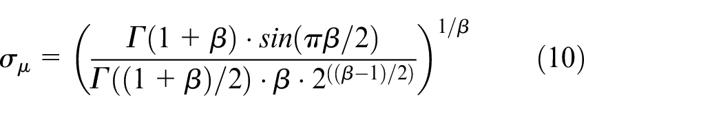
In equation (7), Levy meets the lévy distribution, and Mantegna algorithm can setsthe lévy random step s:

s = \frac{μ}{{| v |}^{(1 / β)}}

(9)

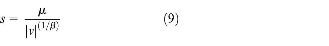
where β is the power-law exponent. µ∼N (0, σ2µ), v∼N (0, σ2v), σ_v = 1, σ_µ can be described as

σ_{μ} = {(\frac{Γ (1 + β) \cdot \sin (π β / 2)}{Γ ((1 + β) / 2) \cdot β \cdot 2^{((β - 1) / 2)}})}^{1 / β}

(10)

Step 3. Update followers positions. Salp followers can change their positions by their neighbors positions. Each salp follower can be expressed as follows

x_{j}^{i} = (x_{j}^{i} + (x_{j}^{i} - F_{j}) Levy) \cdot rand

(11)

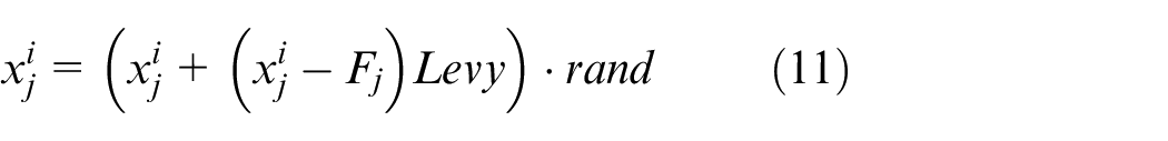
where i ≥ 2, and rand is in the interval of [0, 1].

Step 4. Calculate all fitness values. Select and replace the optimal solution and the best fitness value if there is a better solution, compared with other fitness values. Replace the optimal solution and the best fitness value if there is a better fitness value. Record the global optimum solution and fitness value.

Step 5. Judge whether the optimization circumstances meet the end condition. If no, return to step 2 and go on. Otherwise, stop iterative loops.

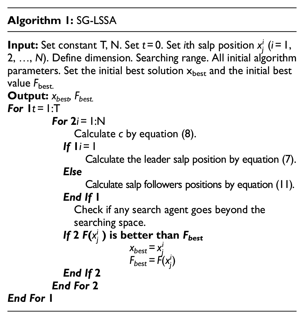
There is the pseudo code for SG-LSSA.

Algorithm 1: SG-LSSA
Input: Set constant T, N. Set t = 0. Set ith salp position $x_{j}^{i}$ (i = 1, 2, …, N). Define dimension. Searching range. All initial algorithm parameters. Set the initial best solution x_best and the initial best value F_best.Output: x_best, F_best.
For 1 t = 1:T For 2i = 1:N Calculate c by equation (8). If 1i = 1 Calculate the leader salp position by equation (7). Else Calculate salp followers positions by equation (11). End If 1 Check if any search agent goes beyond the searching space. If 2 F( $x_{j}^{i}$ ) is better than F_best x_best = $x_{j}^{i}$ F_best = F( $x_{j}^{i}$ ) End If 2 End For 2End For 1

Active disturbance rejection control

Generally speaking, disturbances refer to unexpected changed signals in the system or different physical quantities that cause these changes. Total disturbances can be divided into internal disturbance and external disturbance. The external disturbance refers to the disturbance imposed on the system by the outside environment, such as given disturbance, loading disturbances. The internal disturbance refers to the system internal changes, such as structural changes, the temperature drift, the zero drift, and other parameter changes. In the process of studying system disturbances, ADRC regards the part, including the internal disturbance and the external disturbance, which is different from the standard form in the system dynamics as the total disturbance, and regards the total disturbance as the original system state. Then, the original system state and different disturbances will be estimated and compensated together by using the state observer idea in the modern control theory, which can give the real-time disturbance rejection. In the practical application of the hydraulic quadruped robot, there are a lot of uncertainties in the contact environment, and there are various dynamic nonlinear and uncertain disturbances in the robot walking process, so it is difficult to achieve a satisfactory control effect by using classical control methods. Therefore, this paper proposed the active disturbance rejection control algorithm based on SG-LSSA, which can effectively suppress different disturbances in the external environment and can achieve accurate and stable performance. ADRC uses ESO to observe state variables and internal-external disturbances in the system, which can suppress the adverse effects of time-varying uncertainty. To get feasible ADRC parameters, the ADRC controller is tuned by SG-LSSA, so as to ensure the accurate control tracking. The mixed control method can not only realize the system accurate control performance but also ensure the anti-interference in the system.

ADRC takes the simple integral series type as the standard type, parts of system dynamics that are different from the standard type are regarded as total disturbances. Then, total disturbances are estimated and eliminated by the extended observer in real-time, so that the controlled object which is full of uncertainties and non-linearity is restored to the standard integral series type, which makes the design of control systems change from the complex to the simple. ADRC has three parts, including the Tracking Differentiator (TD), the Extended State Observer (ESO), and the Non-Linear State Error Feedback (NLSEF). TD is applied to get the differential signal of the input signal and arrange the transition procedure. TD can arrange the transition process which has a filtering function. Systems can use the transition process through TD to accelerate the response speed filter the data. ESO can estimate the state variables and internal-external disturbances of systems. NLSEF is used to realize the nonlinear control by combining the error between the transient procedure and the estimated value of state variables. According to the observer idea in modern control theory, ADRC uses the extended state observer to observe the state variables and internal-external disturbances, which can carry on the dynamic compensation to suppress adverse effects caused by time-varying uncertainties and external disturbances. To compensate for the system dynamic time delay, ADRC adopts the loading force compensation methods to compensate for the external loading force which is fed forward to ensure that the given force signal can be accurately tracked. ADRC lumps the effects on the output derived from both external dynamics and disturbances and dynamics, and general nonlinear uncertainties will be permitted in ADRC. Moreover, desired system performances can be met since the total uncertainties are timely compensated for. In this paper, the controlled model is a three-order system, therefore, the ADRC is constructed for the three-order controller, and the ADRC structure block diagram is shown in Figure 4. In Figure 4, x₁ to x₃ are output signals of the TD, z₁ to z₄ are output signals of the NLSEF, e₁ to e₃ are calculated by different between signal x₁ to x₃, and signal z₁ to z₄, the control amount u0 is generated by the non-linear function, b₁ and b₂ are ADRC parameters.

Figure 4.

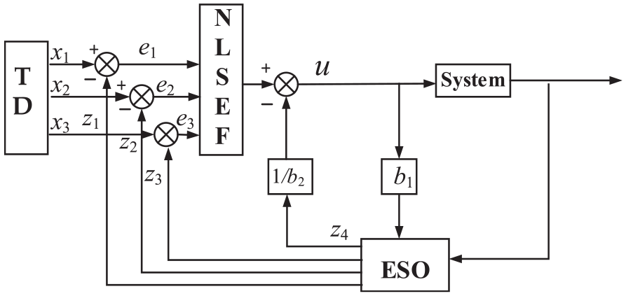
The ADRC structure block diagram.

The discrete ESO model can be given as follows:

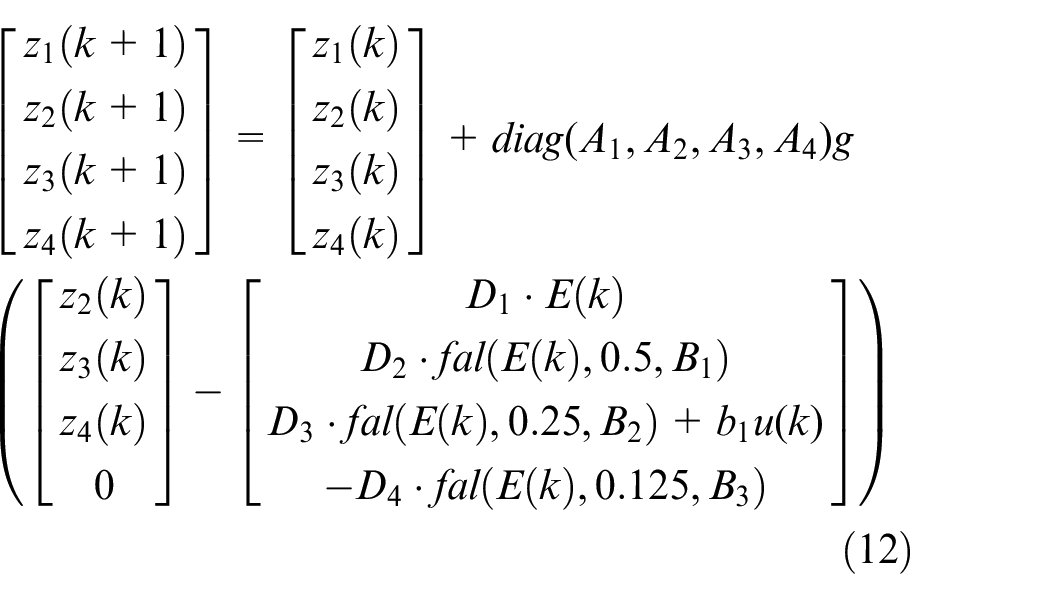
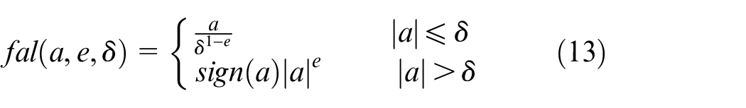
\begin{matrix} [\begin{matrix} z_{1} (k + 1) \\ z_{2} (k + 1) \\ z_{3} (k + 1) \\ z_{4} (k + 1) \end{matrix}] = [\begin{matrix} z_{1} (k) \\ z_{2} (k) \\ z_{3} (k) \\ z_{4} (k) \end{matrix}] + diag (A_{1}, A_{2}, A_{3}, A_{4}) g \\ ([\begin{matrix} z_{2} (k) \\ z_{3} (k) \\ z_{4} (k) \\ 0 \end{matrix}] - [\begin{matrix} D_{1} \cdot E (k) \\ D_{2} \cdot fal (E (k), 0.5, B_{1}) \\ D_{3} \cdot fal (E (k), 0.25, B_{2}) + b_{1} u (k) \\ - D_{4} \cdot fal (E (k), 0.125, B_{3}) \end{matrix}]) \end{matrix}

(12)

where k is the sampling number, E(k) = z₁(k) − y(k), y(k) is the system output signal, A₁ to A₄, D₁ to D₄, and B₁ to B₃ are ESO parameters, b₁ is ADRC parameter, and b₁ = 0, fal is a control function and its definition is as follows:

fal (a, e, δ) = {\begin{matrix} \frac{a}{δ^{1 - e}} \begin{matrix} | a | \leq \end{matrix} δ \\ sign (a) {| a |}^{e} \begin{matrix} | a | > δ \end{matrix} \end{matrix}

(13)

The discrete TD model is given as follows:

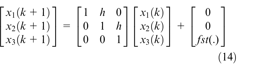
[\begin{matrix} x_{1} (k + 1) \\ x_{2} (k + 1) \\ x_{3} (k + 1) \end{matrix}] = [\begin{matrix} 1 & h & 0 \\ 0 & 1 & h \\ 0 & 0 & 1 \end{matrix}] [\begin{matrix} x_{1} (k) \\ x_{2} (k) \\ x_{3} (k) \end{matrix}] + [\begin{matrix} 0 \\ 0 \\ fst (.) \end{matrix}]

(14)

where h = 1, fst is a control function, and its definition is as follows:

\begin{array}{l} f s t (m_{1}, m_{2}, m_{3}, m_{4}) \\ = {\begin{matrix} - m_{3} \cdot s i g n (m_{5}) & | m_{5} | > m_{3} m_{4} \\ - m_{3} \cdot (m_{5} / m_{3} m_{4}) & | m_{5} | \leq m_{3} m_{4} \end{matrix} \end{array}

(15)

m_{5} = {\begin{matrix} m_{6} = \sqrt{d^{2} + 8 r_{1} | m |} \\ m_{2} + \frac{m_{6} - m_{3} m_{4}}{2} \begin{matrix} sign (m) & | m_{6} | > m_{3} m_{4}^{2} \end{matrix} \\ m_{2} \begin{matrix} + \frac{m_{6}}{m_{4}} & \begin{matrix} \begin{matrix} | m_{6} | \leq m_{3} m_{4}^{2} \end{matrix} \end{matrix} \end{matrix} \end{matrix}

(16)

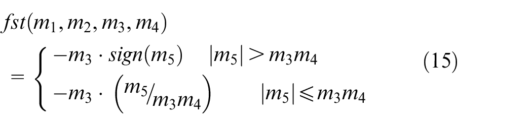
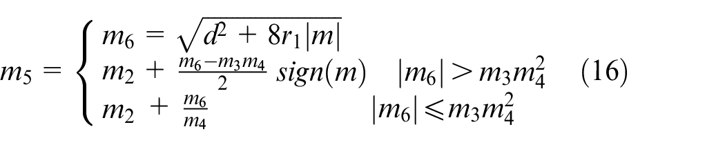
where m₃ and m₄ are TD parameters. m₂ = x₂(k).

The discrete NLSEF model in this paper is given as follows:

u (k) = fst (e_{1} (k), D_{5} e_{2} (k), D_{6}, D_{7}) - z_{4} (k) / b_{2}

(17)

where D₅ to D₇ are ESO parameters, b₂ = 1.

ADRC owns 16 parameters, including D₁ to D₇, A₁ to A₄, B₁ to B₃, m₃ to m₄. ADRC parameters influence system response speed and steady-state errors. Therefore, it is important to get appropriate parameters to have a high controllability system.

The proposed control method

Authors should discuss the results and how they can be interpreted from the perspective of previous studies and of the working hypotheses. The findings and their implications should be discussed in the broadest context possible. Future research directions may also be highlighted.

Evaluation function

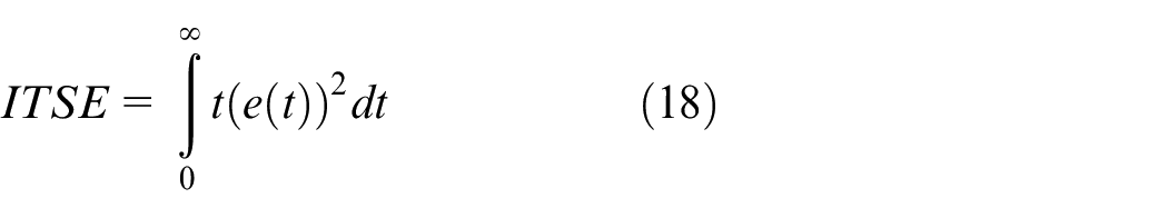
The ADRC parameter finding problem can be transformed into the 16-dimension optimization problem. It is important to choose a feasible evaluation function before optimization. Sixteen parameters can be seen as solutions to the evaluation function. The result of evaluation functions can be seen as measuring performances of systems. The purpose of the tuning method is that the evaluation function is minimized by different algorithms in ADRC. Evaluation functions mainly include the integral of the squared value of error (ISE), the integration of the absolute value of error (IAE), the integral of time multiplied by the absolute value of error (ITAE), the mean of the square of the error (MSE), and the integral of time multiplied by the square value of error (ITSE). IAE and ISE are single objective functions that only consider single factors and cannot reflect hydraulic systems states. IAE only considers the absolute error. ISE only considers the square of the error, so the large error is penalized more than the smaller error, which can cause that systems endure the gradual accumulation of small errors. MSE can weaken the limitations of the ISE by computing the decay probability per second of ISE, but systems need to run for a long time. ITSE owns an additional time for ITAE which penalizes and weighs large errors and it has high speed. ITSE can not only weigh a long time but also penalizes accumulated errors. ITSE can evaluate systems than other functions. ITSE was selected in this paper.

ITSE = \int_{0}^{\infty} t {(e (t))}^{2} dt

(18)

Control method

The ADRC control performance depends on 16 parameters. To get the optimal ADRC, ADRC parameter-tuning problem was converted into a class of 16-dimension optimization problems in this paper. All ADRC parameters can be seen as salp positions in 16-dimensional space. The ITSE is selected as the evaluation function. All salp positions were randomly set, and then all salp positions were input into ADRC as 16 parameters to find the smallest ITSE value. The salp position that minimized the ITSE can be seen as the optimum ADRC parameters and the position that minimized the ITSE was applied to update the optimum ADRC parameters in the next iteration. If the tuning procedure met the maximum number of iterations, the optimal salp position can be seen as the best ADRC parameter. The proposed ADRC working flow chart in Figure 5. The ADRC parameter-tuning steps are as follows

Step 1. Set all initial algorithm parameters. Initially set N salps positions $x_{j}^{i}$ , the maximum number of search iterations T, t = 1. Set the finding range. Each salp position can be seen as the 16 ADRC parameters.

Step 2. Judging whether i is equal to 1. If i is equal to 1, go on to Step 2. If i is not equal to 1, jump to Step 3. Operate the control system. Update c using equation (8). Update the leader position in equation (7). Calculate ITSE in the control system.

Step 3. Operate the control system. Select rand in the range of [0, 1]. Update followers positions using equation (11). Calculate the ITSE of each salp in the control system. Record all ITSE values and find the minimum ITSE value. Replace the optimal salp position and the minimum ITSE value. The salp position which minimizes the ITSE can be considered as the best ADRC parameter.

Step 4. Set t = t + 1.Judge if t = T. If t is equals to T, stop. The global optimum salp position can be selected as the best ADRC parameter. If t is not equal to T, return to Step 2.

Figure 5.

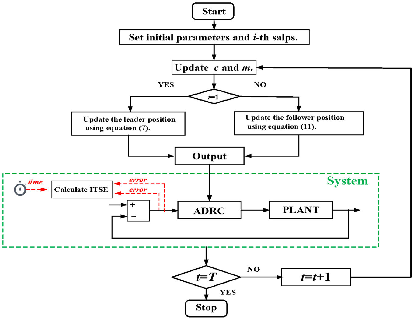
The proposed ADRC working flow chart.

Discussion

The application object

There are four lower computers and one upper computer in systems. Four lower computers have the CAN-BUS module, the A/D module, and the D/A module. The upper computer has the CAN-BUS module and the analog acquisition module. The A/D converter was used to collect the position information and the driving information of hydraulic servo actuators. The D/A converter was used to convert digital control signals into analog signals. The nine-axis inertial navigation system is installed in the robot, which can output the real-time three-axis acceleration, the three-axis angular velocity, the pitching, and the rolling information of the robot body in the Cartesian coordinate system. The constant pressure pump and the accumulator were used to supply the oil. The pump station is equipped with the flow sensor and the oil pressure sensor to monitor the changing of the pressure and the flow in controlled systems, which can provide the basis for the oil source design. The proposed control method was used in the robot joint in the hydraulic quadruped robot developed by the Hydraulic Quadruped Robot Lab at Harbin University of Science and Technology. The servo valve is the SFL212F-12/8-21-40 force-feedback valve made by the 18th Research Institute of the First Academy of China Aerospace Science and Technology Corporation (Beijing, China). The sensor is the LVDT-PA1HL60X sensor made by the Fuxin-Lisheng Automatic Control Co., Ltd. (Fuxin, China). The application object is the knee joint. Each joint driving force in the signal leg is provided by the hydraulic cylinder between two adjacent parts which is adjusted by the servo valve. The pressure and flow through the hydraulic cylinder are throttled to realize the output force control and corresponding motion control in the joint. The joint angle is calculated by the displacement device and the linear displacement sensor installed on the hydraulic cylinder. The robot single-leg measurement and control system is mainly used for the sensor signal acquisition and the servo valve control signal output. The control signal is got by the industrial control software, and then the control signal will be inputted to the servo valve amplifier through the D/A module of the data acquisition card to drive the hydraulic cylinder operation. Output signals of the displacement sensor and the force sensor on the hydraulic cylinder are inputted to the acquisition card through the signal conditioning circuit A/D module, and finally to the industrial computer software.

This paper used different ADRC controllers based on different algorithms to display control performances. All system models were simulated and built-in MATLAB. All algorithms have SG-LSSA, bat algorithm (BA),⁴³ cuckoo search algorithm (CS),⁴⁴ and simulated annealing (SA).⁴⁵ The application object was shown in Figure 6.

Figure 6.

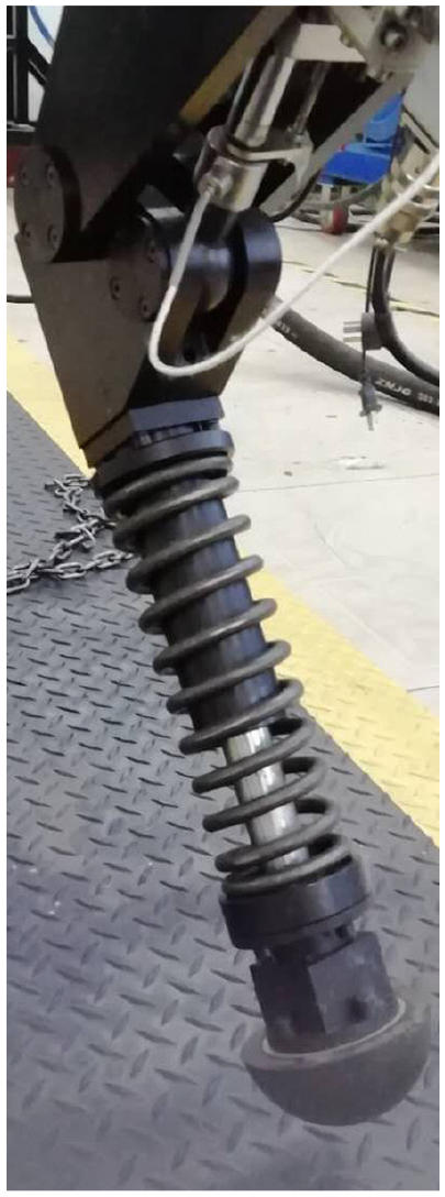
The application object.

For assumptions and constraints of 16 parameters in the ADRC controller, there can be divided into three parts. For ESO, reasonable parameters can make that ADRC can better track the status and unknown perturbations of the controlled system, and the tracking efficiency of ESO is higher, the ADRC efficiency is better. Parameters D1 to D4 are determined by the sampling step size of the system, the sampling step size of the system usually in the range of [0,1]. So parameters D1 to D4 do not needs to have a large scope, and this paper makes D1 to D4 in the range of [0, 10]. For TD, if output signals of TD can track the input signal accurately, the parameter tuning effect is gratifying. The control gain is determined by the required speed of the transition process and affordabilities of the system. It is important to deal with the transition procedure requirements. For NLSEF, the compensation factor b2 is the main parameter affecting ADRC performances. In practical application, the compensation factor b2 can be approximately estimated as a constant one, can be treated as an approximate disturbance. So, the control gain is larger, the transition arrangement is shorter, other ADRC parameters in the range of [0, 100000]. Parameter h is usually a multiple of the sampling period by a factor of at least four in the ADRC basic literature.¹⁹ This paper select h = 1 because the sampling period is in the range of [0.01, 0.25]. The parameter b₁ is the ESO Output weight, and the disturbance component can be reduced by reducing the z₄ signal. To make ESO work effectively, the parameter b₁ should be known or close to the actual value before the optimization process. If the accurate value of the parameter b₁ cannot be obtained, it can be replaced by its approximate estimation. In this way, the system can deal with the z₄ signal into a part of disturbances. So this paper select b₁ equal to 1 to reduce the system computation. In the ADRC basic literature,¹⁹ too large or too small b₂ will enhance ESO disturbances. So it is important to set the appropriate b₂ according to bearing system capacities to weaken the system overshoot and the unnecessary energy loss. When the controlled system changing is not very drastic, the parameter b₂ can be equal to 0 to simplify the controller structure.

The earliest idea of the SA was proposed in the early 1980s. It is a stochastic optimization algorithm based on the Monte Carlo method. SA was inspired by the solid matter annealing process in physics. First, the solid is heated to a sufficiently high temperature and then is cooled slowly. During the heating process, all particles in the solid will become disordered with the temperature rising, and the internal energy will increase. When all particles gradually are cooled down. SA starts from a certain initial temperature and combines with the characteristic of probability jumping to search for all feasible solutions in objective functions. SA has two Initial parameters including the initial temperature T and the decay factor k. For SA, parameter T was selected 100, k was selected as 0.95.

BA is a heuristic algorithm was proposed by Professor Yang in 2010. BA simulates bats using the sonar to detect animals and avoid obstacles in nature. The bionic principle of BA maps bat individuals into feasible solutions in the searching dimension. BA mainly includes the individual moving process and the hunting process. The fitness function value in BA is applied to measure the bat position. The survival of the fittest in the process will be compared to the iteration process of replacing the poor feasible solution with a good feasible solution in the searching process. In BA, the loudness coefficient equals to 0.9, the rate coefficient equals to 0.9, and the pulse frequency was selected in the range of [0, 1].

CS was proposed by Professor Xin She Yang and Suash Deb in 2009. Cs mainly has two strategies including the cuckoo nest parasitism method and the levy flight mechanism. Cuckoo will use the random walking method to get an optimal nest to hatch their eggs, which can achieve an efficient optimization model. CS uses egg nests to represent solutions. In the simplest case, each nest has an egg, and each cuckoo egg represents a new solution, and the aim in CS is to apply good solutions to replace bad solutions. The probability factor is 0.25, and the power-law exponent is 1.5.

For the SG-LSSA the power-law exponent is 1.5. All initial algorithm parameters were selected according to basic algorithm literature, and all algorithm details can be found in basic algorithm literature. ITSE was selected as the evaluation function. Set maximum iterations 500. Set population size 50. Set D₁ to D₄ in the range of [0, 10]. Set other parameters in the range of [0, 100000].

Time domain analysis

Filtering analyses, amplification analyses, statistical characteristic analyses, and other analyses of signals are called the time domain analysis, depending on the temporal response and response curves. The time-domain analysis uses the time as the independent variable to describe changes of signals, which is the most basic and intuitive expression in system performances. Time-domain analysis can effectively enhance the signal-to-noise ratio, obtain the signal similarity and the correlation at different times, get characteristic parameters reflecting the system running state, which can provide effective information for the dynamic analysis and the fault diagnosis of systems. System signal changed processes are called the temporal response in different input signals. There are two parts in the temporal response, including the transient response and the steady-state response. The transient response means that output signals are changed from the initial state into the final stable state in different input signals. There are four indices in the transient response, including overshoot M, delay time t_d, peak time t_p, settling time t_s. The ratio of the instantaneous maximum deviation of the steady-state value under the step signal is called the overshoot. Delay time is that the system running time makes the output signal reach the half-steady state value. Peak time is the system running time make the output signal reach the maximum value. The setting time means the shortest time which makes the system return to the new equilibrium state in interference environments, and the error range is 5%–2% of the steady-state value. The steady-state response means the system outputting state in an infinite time, and the factor es determines the difference between the final signal and the ideal signal.

Table 1 shows temporal response factors and ITSE values for different algorithms. For the steady-state response, SG-LSSA-ADRC has the smallest of the steady-state error, which can reverse that the proposed controller can weaken oscillatory harmonics and eliminate the strong pulse wave. For the transient response, the ADRC controller tuned by the SG-LSSA gets the smallest overshoot, settling time, and delay time. BA-ADRC has the smallest peak time. Although the peak time of BA-ADRC is lower than that of the SG-LSSA-ADRC, the difference range is 0.001 s, which can be negligible. Good transient response indices provide positive dynamic stability and the well-damped to disturbances. For the system evaluation equation, the designed method has the smallest ITSE in algorithms. It is a clear show that SG-LSSA owns good global iteration performance and accuracy in comparison with other algorithms that are easy to be trapped in the local solution. The proposed algorithm can give the distinguished finding ability and avoid prematurity, and its precision ability ranks first in all algorithms. The temporal response shows that the SG-LSSA-ADRC has excellent dynamic and static flat horizontal and stable performance under the step signal. ITSE value means that SG-LSSA has a wide adjustment range, high efficiency, and good effect.

Table 1.

Temporal response factors and ITSE.

Algorithm	e_s	M	t_d	t_p	t_s	ITSE
SG-LSSA	2.42E-04	0.038	0.058	0.083	0.071	1.61E-03
SA	0.002	0.118	0.063	0.098	0.164	1.12E-03
BA	3.00E-04	0.110	0.058	0.082	0.094	1.07E-03
CS	3.72E-04	0.183	0.062	0.087	0.109	1.10E-03

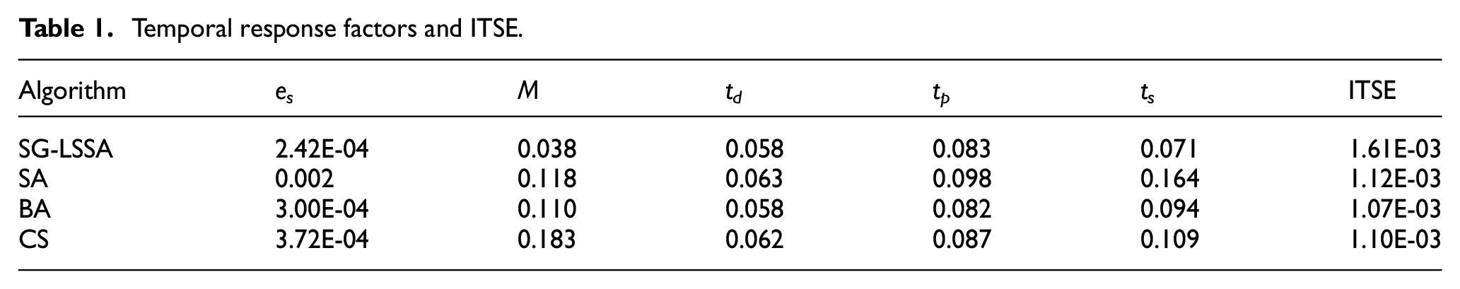
Two-dimension step response curves and three-dimension step response curves were shown in Figure 7. The unit for the amplitude is the angle (°). CS-ADRC and SA-ADRC own large overshoot, and SA-ADRC has the oscillation phenomenon in the later response phase. As time goes by, the SA-ADRC controller will make system damage and degradation. The overshoot of the ADRC derived by BA is lower than those of CS-ADRC and SA-ADRC but is larger than SG-LSSA-ADRC. Although SG-LSSA-ADRC owns some overshoot, the proposed controller will weaken the overshoot into the ideal signal value. The step response curve of the proposed controller converges to the ideal value with the minimum overshoot. When the proposed controller is used, the system can keep high precision and perfect dynamic characteristics, showing good robustness and practicability. For the error and the accuracy in the time domain analysis, we can see that the proposed method has the smallest error and the largest accuracy in Table 1. In the Figure 7, the proposed ADRC control signal is closest to an ideal input signal, and the adjustment process is more stable and shorter, and the response rate is faster, so the proposed method has a strong self-adjustment ability and a good effect.

Figure 7.

Step response curves: (a) two dimension curves and (b) three dimension curves.

Frequency domain analysis

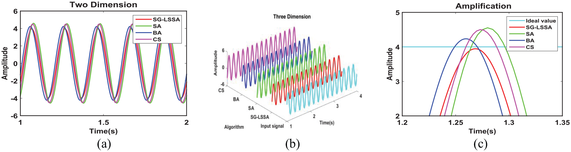
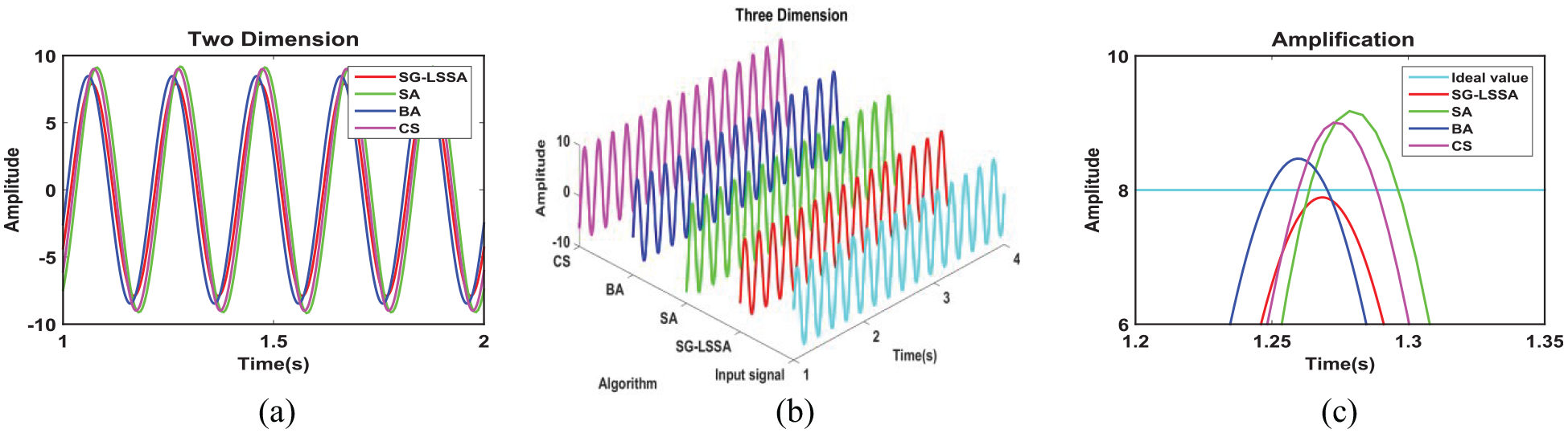
The frequency response is the system response performance in sinusoidal signals. For the ideal system, the system output signal is still the same frequency sinusoidal signal when the sinusoidal signal is entered. According to the frequency response, the system’s ability to reproduce signals and filter noise can be evaluated intuitively. The frequency response factor includes the amplitude-frequency characteristic that shows the relationship between the gain and the signal frequency. If the output amplitude is closer to the input amplitude, the system has a better frequency response. To show the mechanical impedance and stiffness of the proposed controller, different sinusoidal signals were input into controlled systems. For different sinusoidal signals, different angular velocities were 5π and 10π, the phase was zero, different amplitudes were 4, 8, and 12. All response results including two-dimensional response curves, three-dimensional response curves, and the local amplification are shown in Figures 8 to 13. As we can see in Figures 8 to 13, the amplitude of SG-LSSA-ADRC controller is closest to the ideal amplitude, amplitudes of ADRC except that of SG-LSSA-ADRC are larger than the ideal value and the system controlled by SA-ADRC has the largest amplitude difference between the actual amplitude and the ideal amplitude. Figures mean that the proposed controller has a good ability to keep balance and weaken the non-linear error in different signals combined with noise and interference. SG-LSSA-ADRC has a good sinusoidal waveform and perfect loading characteristics. For the error and the accuracy in the frequency domain analysis, we can see that see all signals of SG-LSSA-ADRC controllers are closest to the ideal signal in Figures 8 to 13. All signals of SA-ADRC controllers have maximum signal distortion performances. When loadings are changed, the proposed ADRC control can adjust the control signal effectively and can keep good control performance. So the proposed control method has the smallest error and the best accuracy in the Frequency Domain Analysis.

Figure 8.

Sinusoidal response curves of amplitude 4 and angular velocity 5π: (a) two dimension curves, (b) three dimension curves, and (c) amplification curves.

Figure 9.

Sinusoidal response curves of amplitude 4 and angular velocity 10π: (a) two dimension curves, (b) three dimension curves, and (c) amplification curves.

Figure 10.

Sinusoidal response curves of amplitude 8 and angular velocity 5π: (a) two dimension curves, (b) three dimension curves, and (c) amplification curves.

Figure 11.

Sinusoidal response curves of amplitude 8 and angular velocity 10π: (a) two dimension curves, (b) three dimension curves, and (c) amplification curves.

Figure 12.

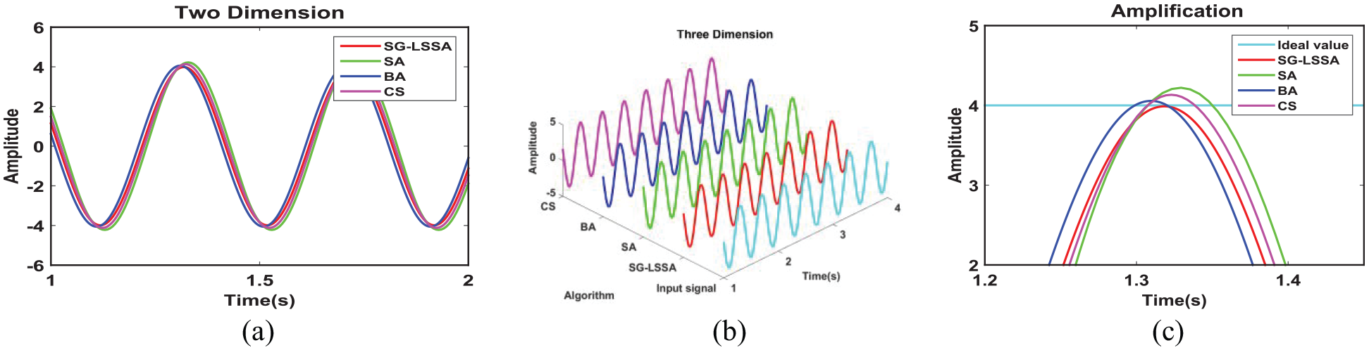
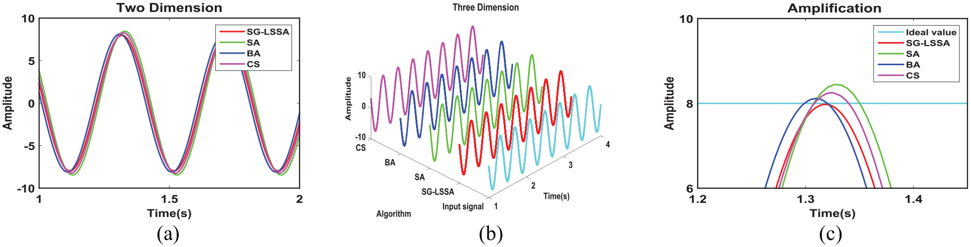
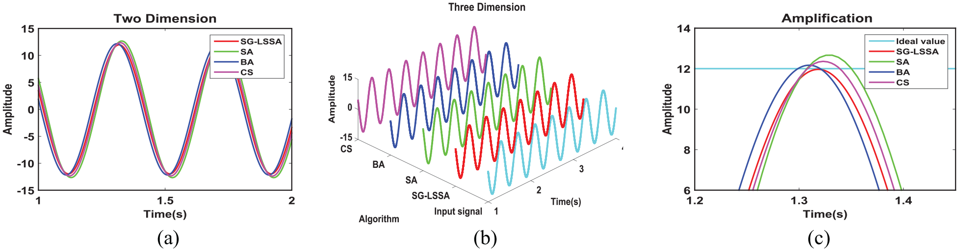
Sinusoidal response curves of amplitude 12 and angular velocity 5π: (a) two dimension curves, (b) three dimension curves, and (c) amplification curves.

Figure 13.

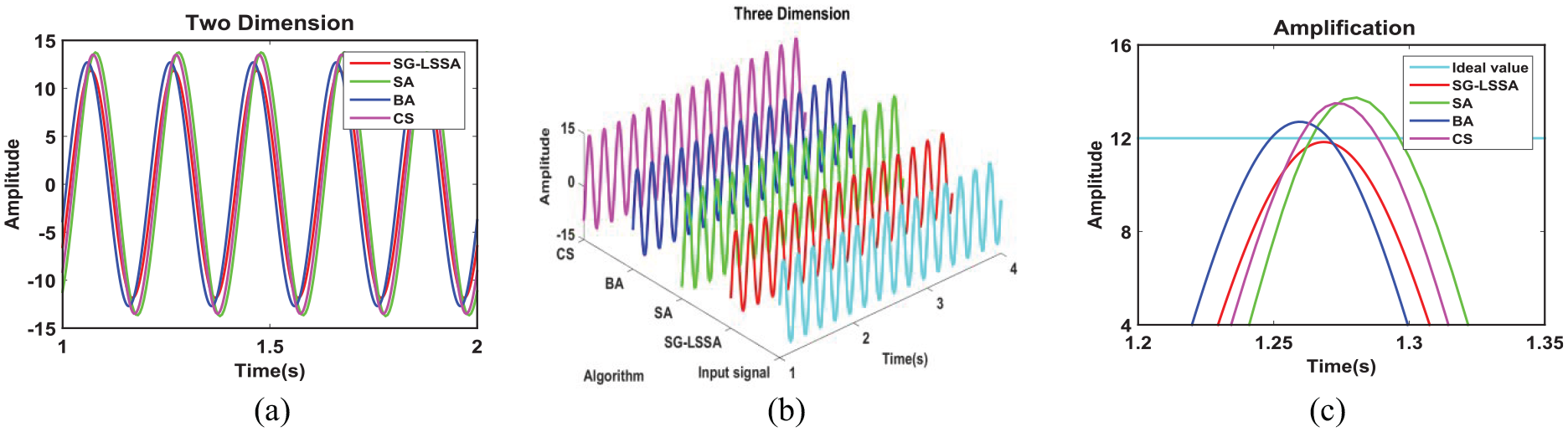
Sinusoidal response curves of amplitude 12 and angular velocity 10π: (a) two dimension curves, (b) three dimension curves, and (c) amplification curves.

Sawtooth response analysis

To further show the reliability of the SG-LSSA-ADRC, two-dimensional response curves, and three-dimensional response curves based on different algorithms are presented in Figures 14 and 15 when input signals are different sawtooth signals. Figures showed that the SG-LSSA-ADRC has the smallest amplitude error, the highest response speed, the least shock. BA-ADRC has the largest vibration and signals distortion. Because collected signals in BA-ADRC contain noises and weakened, the signal distortion should be processed. Figures 14 and 15 indicate that the proposed controller can not only weaken the vibration signal but also improve dynamic and static performances. The system owns an exceptional ability to keep the balance and cut down the concussion strength when the proposed controller is applied. The system owns an exceptional ability to keep the balance and cut down the concussion strength when the proposed controller is applied, which can ensure that the system performance gets long-term high efficiency. In other words, the SG-LSSA-ADRC has anti-jamming performance and can boost the curious equity of the hydraulic robot in different environments. For the error and the accuracy in the sawtooth response analysis, we can see that see all signals of SG-LSSA-ADRC controllers has the least signal oscillation and distortion. All signals of BA-ADRC controllers have the largest error and the smallest accuracy. The system using the proposed control method can restrain the external disturbance and remove the noise, and sawtooth response curves are relatively smooth. For different sawtooth signals, the changing trend of each curve in the proposed controller is similar, which further shows that the SG-LSSA-ADRC has less influence on the system performance, and can maintain good steady-state precision and dynamic characteristics.

Figure 14.

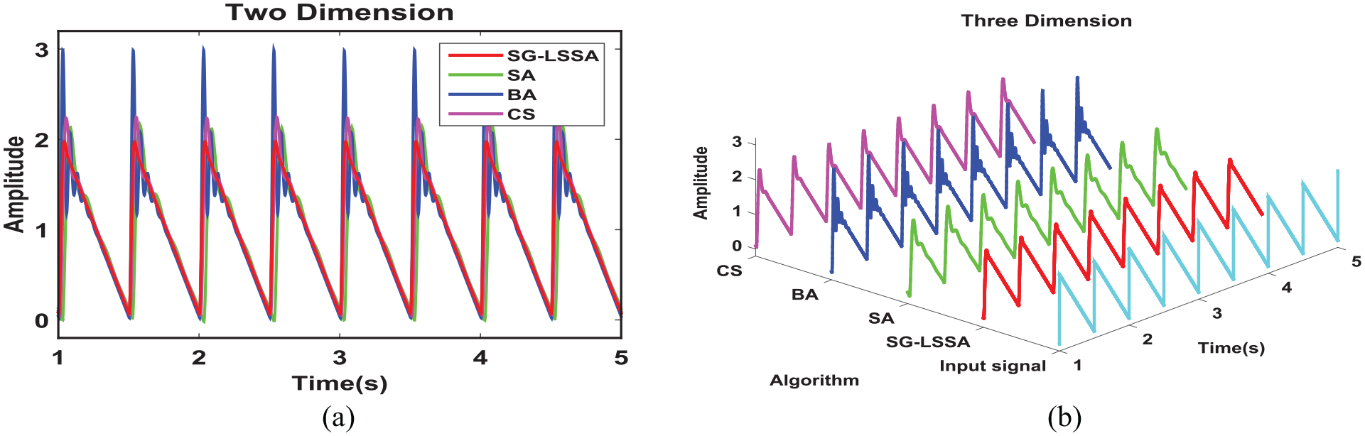
Sawtooth response curves 1: (a) two dimension curves and (b) three dimension curves.

Figure 15.

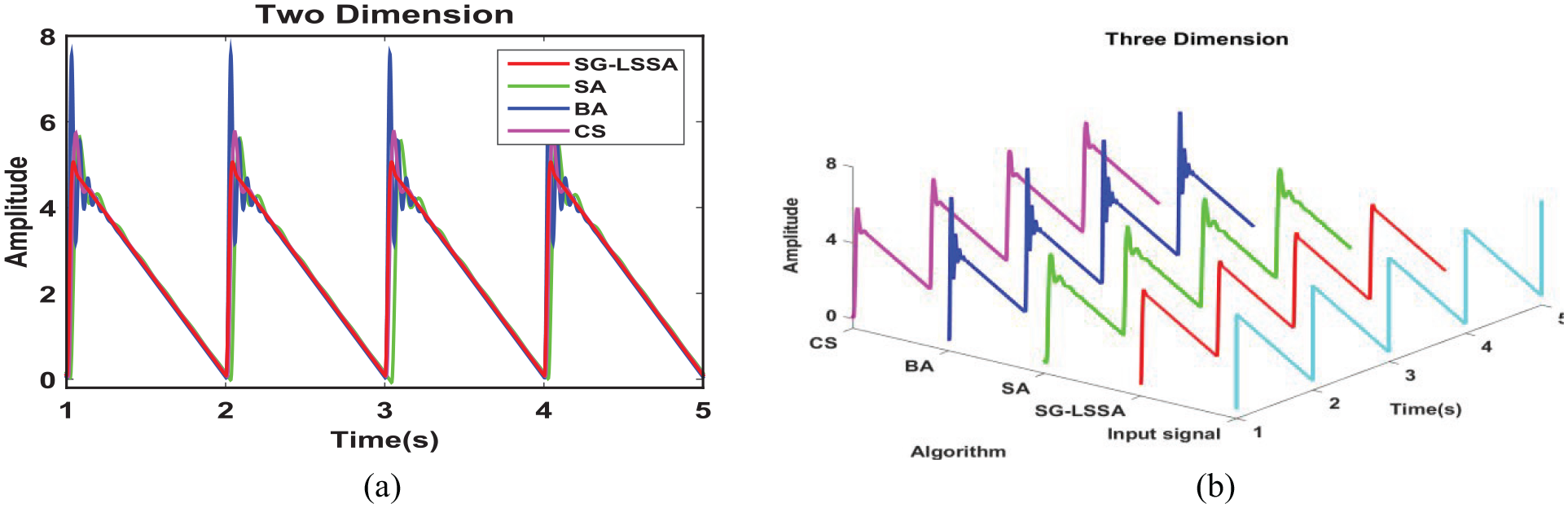
Sawtooth response curves 2: (a) two dimension curves and (b) three dimension curves.

Ramp response analysis

The ramp signal is zero at the negative half axis and is a positive proportion function at the positive half axis. When the slope is 1, it is called the unit ramp signal. The ramp signal is a testing signal which is used to study the system model and the fed system relating information in system dynamics. To study the track precision and the orientation precision of the system, different ramp signals were chosen as the testing signal. And slopes were separately selected 5 and 100. The result was shown in Figures 16 and 17. From Figures 16 and 17, we can see that the system goes to steady-state gradually with the lowest response speed and the largest error under SA-ADRC. When the signal slope increases gradually, the difference between the actual signal and the ideal value is increasing, and the difference of SG-LSSA-ADRC is the smallest in all controllers. Ramp response results display that the proposed controller has a better tracking performance than the other three controllers in this paper, which mainly reflects in expanding the range of the signal slope, the response precision, and systemic stability, and can eliminate under-compensation and over-compensation. For the error and the accuracy in the ramp response analysis, we can see that see all signals of SG-LSSA-ADRC controllers not only has the shortest distance from stability curves and ideal curves, but also has the minimum signal turbulence. SG-LSSA-ADRC controller can not only can enhance the stability and tracking accuracy, but also expand the frequency response of the system. So SG-LSSA-ADRC controller has the high robust performance and the anti-interference ability.

Figure 16.

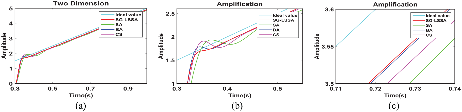
Ramp response curves 1: (a) two dimension curves, (b) amplification curves 1, and (c) Amplification curves 2.

Figure 17.

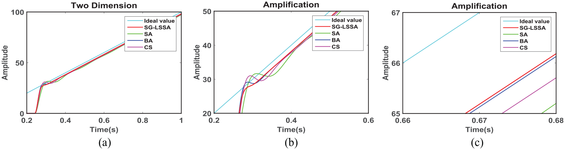
Ramp response curves 1: (a) two dimension curves, (b) amplification curves 1, and (c) amplification curves 2.

Random response analysis

To test the anti-interference ability of the proposed controller, the response curves of the system under different ADRC controllers were presented in Figures 18 and 19 when interference signals were random signals. Response results include two-dimensional response curves and three-dimensional response curves. The response curve of the proposed controller is closest to the ideal curve and has the smallest peak shock. For random signals, the SG-LSSA-ADRC owns an exceptional efficiency to keep the system balance and weaken the shaking, and the achievement of the controlled system is undisturbed by extraneous interferences. SA-ADRC and CS-ADRC have large static state error, can not keep smooth in the signal peaking time, and output signals give large converting waves when signal size and direction are changed. Using the proposed controller, the robot system can retain strong stability characteristics and can display good robustness, practicability, and accuracy. For the error and the accuracy in the random response analysis, we can see that see all signals of SG-LSSA-ADRC is closest to input curves. All signals of SA-ADRC have excessive amplitudes, have the largest error and the worst accuracy. With the proposed strategy, the control system can realize the smooth operation and the strong precision positioning. So the designed control strategy can satisfy the control operation and accomplish specific working tasks in the hydraulic quadruped robot.

Figure 18.

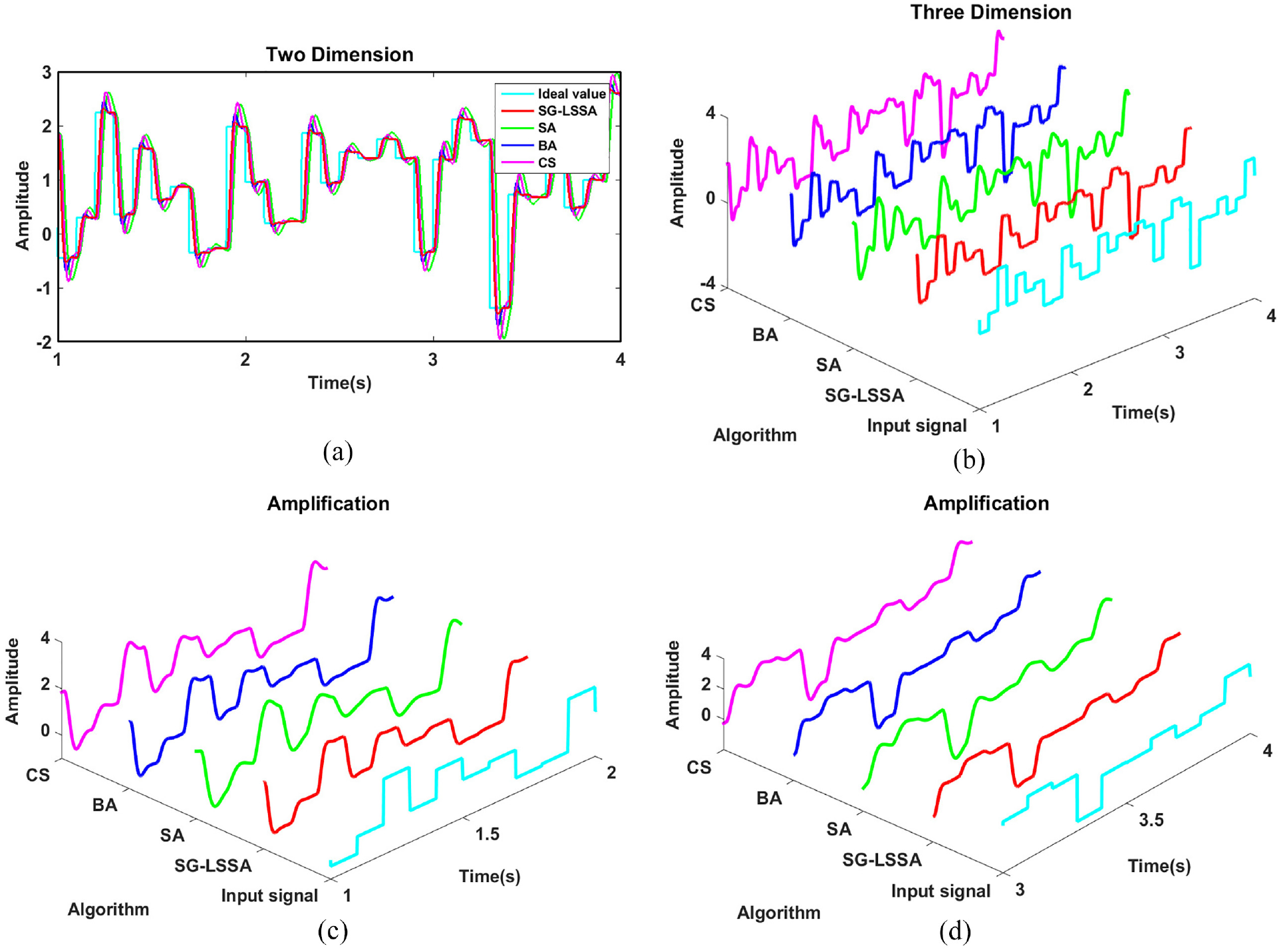
Random response analysis 1: (a) two dimension curves, (b) three dimension curves, (c) amplification curves 1, and (d) amplification curves 2.

Figure 19.

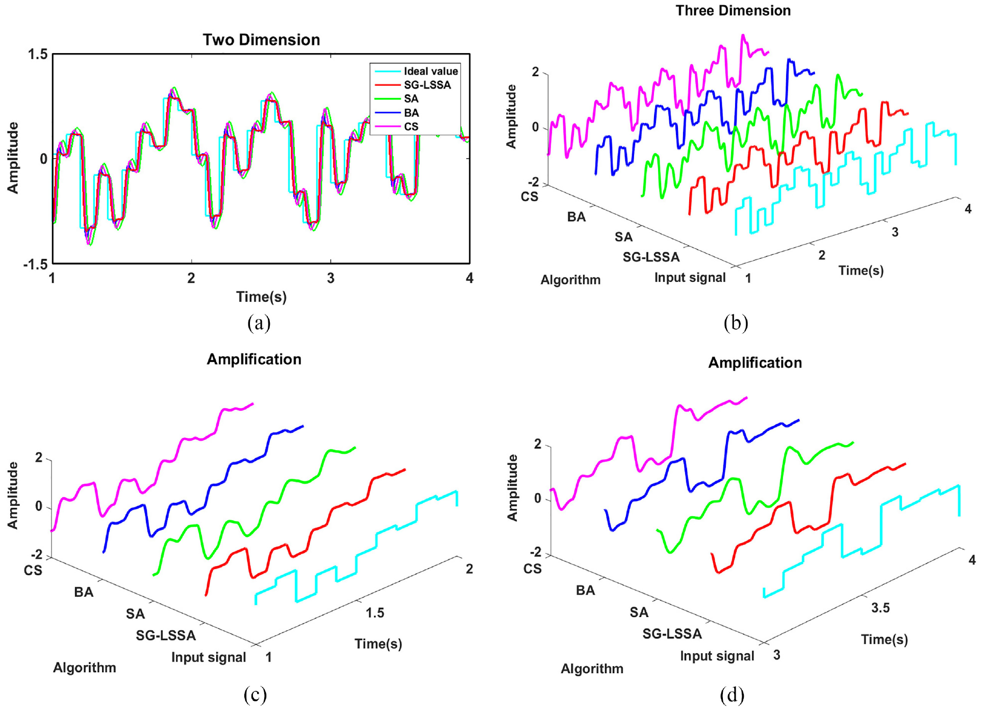
Random response analysis 2: (a) two dimension curves, (b) three dimension curves, (c) amplification curves 1, and (d) amplification curves 2.

Conclusions

This paper used the self-growing lévy-flight salp swarm algorithm to find appropriate ADRC parameters and applied the proposed controller to the joint system of a hydraulic quadruped robot. The SG-LSSA is a hybrid algorithm based on the self-growing method and the lévy flight salp swarm algorithm has good convergence ability. ADRC is a nonlinear control method that aims to create controller law for nonlinear uncertain systems. The ADRC not only mixes different cognitions of the modern control theory with the modern signal processing technology but also inherits the advantages of the PID controller. The proposed ADRC controller automatically detects the real-time error and the external disturbances, then automatically keeps the robustness and balance, which can satisfy different requirements of the joint control system in the hydraulic quadruped robot. Firstly, a hydraulic system mathematical model was got through the literature and theoretical analysis. Then, this paper converted the ADRC parameters tuning problem into the numerical optimization problem, and 16 ADRC parameters can be seen as the 16 dimension searching solution. ITSE was selected as the system evaluation function. Third, Different algorithms including BA, CS, and SA were used in systems to find ADRC parameters to show the performance of the proposed controller. Finally, the step signal, the sinusoidal signal, the sawtooth signal, the ramp signal, and the random signal have entered the system to test different abilities of the proposed controller under different interference signals. The step response results show that the SG-LSSA-ADRC has the smallest overshoot, and can effectively improve the system dynamic characteristics. The sinusoidal response results show that the output amplitude of the proposed controller is closest to the ideal amplitude, which means that SG-LSSA-ADRC can weaken the oscillation and shaking phenomenon. The sawtooth response results show that the proposed controller has the smallest distortion. All testing results showed that the proposed ADRC controller has good performance in the join systems.

The initial leader step is added a larger value in SG-LSSA to obtain a better leader position and a faster speed. As iterations continue, the leader step gradually obtains some good feasible solutions, and the leader searching step can be changed from large to small. So the proposed method can give the relatively accurate ADRC parameter. The controlled system having the proposed method can maintain the wonderful tracking characteristic. These results identify that the SG-LSSA-ADRC controller has a good response performance. Because there are 16 parameters in the third-order ADRC controller, the ADRC parameters searching problem is the high dimensional optimization problem which has many local optimization solutions. Problem complexities and the running time will enhance exponentially with the increasing of dimensions when high dimension functions are calculated. So disadvantages of the proposed method is that the control method may cause long start-up and running time in the hydraulic quadruped robot. To weaken disadvantages and comprehensively enhance control performances of the proposed method, in the future we will introduce new algorithms, change the ADRC controller structure, and simplify ADRC parameters.

Based on the proposed controller and obtained testing results in this paper, there are two approaches. One part is to design a compound control strategy combining other controllers with ADRC, which fully applies the advantages of other controllers and control methods to enhance the robustness and the accuracy of ADRC controllers. Another part is to use different algorithms or develop new hybrid algorithms to enhance searching performances of metaheuristic algorithms, if the searching precision of the algorithm is higher, the result of ADRC parameter optimization is better. Two further approaches can meet different control requirements of the synchronization, the precision, and the dynamic compliance in the hydraulic quadruped robot. In future works. We will design the new ADRC controller combining with other control methods to enhance basic ADRC controller performances. And we will design the new hybrid algorithm to further improve the SSA searching accuracy, so we can get a better ADRC parameter optimization result. Finally, we will use new ADRC controller in the leg joint of the hydraulic quadruped robot to get a more satisfactory control effect.

Footnotes

Declaration of conflicting interests

The author(s) declared no potential conflicts of interest with respect to the research, authorship, and/or publication of this article.

Funding

The author(s) disclosed receipt of the following financial support for the research, authorship, and/or publication of this article: This research was funded by the International Cooperation Project (Grant No. 2012DFR70840).

ORCID iD

Yuqi Fan

References

Gao

, et al. Dynamic compliance analysis for LHDS of legged robot, part B: force-based impedance control. IEEE Access 2018; 6: 74799–74811.

Chen

Rong

, et al. A compliant control method for robust trot motion of hydraulic actuated quadruped robot. Int J Adv Robot Syst 2018; 15: 1–16.

Yang

Zhou

, et al. Energy efficient foot trajectory of trot motion for hydraulic quadruped robot. Energies 2019; 12: 2514.

Zhang

. Joint torque and velocity optimization for a redundant leg of quadruped robot. Int J Adv Robot Syst 2017; 14: 1–12.

Ren

Shao

Sun

, et al. The complex dynamic locomotive control and experimental research of a quadruped-robot based on the robot trunk. Appl Sci 2019; 9: 3911.

Shao

Jin

Wang

, et al. Study on motion analysis and force/position hydraulic control of a parallel cylinder transmission system of heavy-duty quadruped robot. Int J Adv Robot Syst 2019; 16(1): 10.

Pan

Chang

Zhang

. Event-triggered adaptive control for uncertain constrained nonlinear systems with its application. IEEE Trans Ind Inform 2020; 16: 3818–3827.

Ding

Liu

Zhao

. A new hydraulic synchronous scheme in open-loop control: load-sensing synchronous control. Meas Control 2020; 53(1-2): 119–125.

Guo

Wang

Liu

. Antiwindup control of an electrohydraulic system with load disturbance and modeling uncertainty. IEEE Trans Ind Inform 2018; 14: 3097–3108.

10.

Wang

Shen

, et al. Nonlinear differential and integral sliding mode control for wave compensation system of ship-borne manipulator. Meas Control 2021; 54(5-6): 711–723.

11.

Pan

Jing

Sun

, et al. A bioinspired dynamics-based adaptive tracking control for nonlinear suspension systems. IEEE Trans Control Syst Technol 2018; 26: 903–914.

12.

Gao

Shao

Yang

. A compound control strategy combining velocity compensation with ADRC of electro-hydraulic position servo control system. ISA Trans 2014; 53: 1910–1918.

13.

Guo

Wang

. Finite-time convergent control of electrohydraulic velocity servo system under uncertain parameter and external load. IEEE Trans Ind Electron 2019; 66: 4513–4523.

14.

Pan

Sun

. Nonlinear output feedback finite-time control for vehicle active suspension systems. IEEE Trans Ind Inform 2019; 15: 2073–2082.

15.

Yang

Liu

Zhang

. A loading control strategy for electric load simulator based on new mapping approach and fuzzy inference in cerebellar model articulation controller. Meas Control 2019; 52(1-2): 131–144.

16.

Liu

Han

, et al. Research on structure decoupling of passive electro-hydraulic force servo system. Adv Mech Eng 2018; 10: 1–11.

17.

Jia

Zhang

Zheng

. Numerical investigation on the effect of hot running rim seal clearance on hot gas ingestion into rotor-stator system. Appl Therm Eng 2019; 152: 79–91.

18.

Pan

Sun

, et al. Adaptive Fault-tolerant compensation control and its application to nonlinear suspension systems. IEEE Trans Syst Man Cybern Syst 2020; 50: 1766–1776.

19.

Han

. From PID to active disturbance rejection control. IEEE Trans Ind Electron 2009; 56: 900–906.

20.

Huang

Cen

. Research on variable mass control of series manipulator based on linear active disturbance rejection control. Meas Control 2020; 53(7-8): 1194–1202.

21.

Long

Cong

, et al. Active disturbance rejection control based human gait tracking for lower extremity rehabilitation exoskeleton. ISA Trans 2017; 67: 389–397.

22.

Wang

Hou

, et al. Passivity-based control for rocket launcher position servo system based on improved active disturbance rejection technology. Adv Mech Eng 2018; 10: 1–11.

23.

Feng

Guo

B-Z

. A new active disturbance rejection control to output feedback stabilization for a one-dimensional anti-stable wave equation with disturbance. IEEE Trans Automat Contr 2017; 62: 3774–3787.

24.

Fang

Yuan

Liu

. Active–disturbance–rejection–control and fractional–order–proportional–integral–derivative hybrid control for hydroturbine speed governor system. Meas Control 2018; 51(5-6): 192–201.

25.

Shao

Liao

Zhang

. Parameter tuning of active disturbance-rejection controller for induction motor based on time scale. Control Theory & Applications 2008; 25: 208–209.

26.

Zhu

. Dynamic parameter setting and application of active disturbance rejection controller. Journal of North China Electric Power University 2005; 32: 9–13.

27.

Xia

. On linear/nonlinear active disturbance rejection switching control. Zidonghua Xuebao 2012; 42: 202–212.

28.

Zhang

Duan

Yang

. Active disturbance rejection control for small unmanned helicopters via levy flight-based pigeon-inspired optimization. Aircr Eng Aerosp Technol 2017; 89: 946–952.

29.

Kang

Wang

Ren

, et al. Optimization design and application of active disturbance rejection controller based on intelligent algorithm. IEEE Access 2019; 7: 59862–59870.

30.

Cai

Lou

Zhao

, et al. Quadrotor trajectory tracking and obstacle avoidance by chaotic grey wolf optimization-based active disturbance rejection control. Mech Syst Signal Process 2019; 128: 636–654.

31.

Yin

Zhang

, et al. Research on active disturbance rejection control with parameter autotune mechanism for induction motors based on adaptive particle swarm optimization algorithm with dynamic inertia weight. IEEE Trans Power Electron 2019; 34: 2841–2855.

32.

Wang

Yang

Jiao

, et al. Design of auto disturbance rejection controller for train traction control system based on artificial bee colony algorithm. Measurement 2020; 160: 1–9.

33.

Hai

Wang

Feng

, et al. Mobile Robot ADRC with an automatic parameter tuning mechanism via modified pigeon-inspired optimization. IEEE/ASME Trans Mechatron 2019; 24: 2616–2626.

34.

Wei

Zhao

Fan

, et al. Parameter tuning of active disturbance rejection control based on ameliorated shark smell optimization algorithm. Control and Decision 2019; 34: 816–820.

35.

Mirjalili

Gandomi

Mirjalili

, et al. Salp swarm algorithm: a bio-inspired optimizer for engineering design problems. Adv Eng Softw 2017; 114: 163–191.

36.

Gao

Hou

Zhang

, et al. An efficient approximation for Nakagami-mquantile function based on generalized opposition-based quantum salp swarm algorithm. Math Probl Eng 2019; 2019: 1–13.

37.

Xing

Jia

. Multilevel color image segmentation based on GLCM and improved salp swarm algorithm. IEEE Access 2019; 7: 37672–37690.

38.

Malhotra

Sappal

. SSA optimized digital pre-distorter for compensating non-linear distortion in high power amplifier. Telecommun Syst 2019; 72: 179–188.

39.

Wan

Mao

Zhou

, et al. A novel nature-inspired maximum power point tracking (MPPT) controller based on SSA-GWO algorithm for partially shaded photovoltaic systems. Electronics 2019; 8: 680.

40.

Yang

Zhong

Zhang

, et al. Novel bio-inspired memetic salp swarm algorithm and application to MPPT for PV systems considering partial shading condition. J Clean Prod 2019; 215: 1203–1222.

41.

Zhao

Yin

. A quadratic penalty item optimal variational mode decomposition method based on single-objective salp swarm algorithm. Mech Syst Signal Process 2020; 138: 1–12.

42.

Fan

Shao

Sun

, et al. Proportional–integral–derivative controller design using an advanced Lévy-flight salp swarm algorithm for hydraulic systems. Energies 2020; 13: 459.

43.

Yang

Hossein Gandomi

. Bat algorithm: a novel approach for global engineering optimization. Eng Comput 2012; 29: 464–483.

44.

Gandomi

Yang

Alavi

. Cuckoo search algorithm: a metaheuristic approach to solve structural optimization problems. Eng Comput 2013; 29: 17–35.

45.

Bohachevsky

Johnson

Stein

. Generalized simulated annealing for function optimization. Technometrics 1986; 28: 209–217.

Improved active disturbance rejection control with the optimization algorithm for the leg joint control of a hydraulic quadruped robot

Abstract

Keywords

Introduction

The hydraulic quadruped robot system

Self-growing lévy-flight salp swarm algorithm

Active disturbance rejection control

The proposed control method

Evaluation function

Control method

Discussion

The application object

Time domain analysis

Frequency domain analysis

Sawtooth response analysis

Ramp response analysis

Random response analysis

Conclusions

Footnotes

Declaration of conflicting interests

Funding

ORCID iD

References