Sage Journals: Discover world-class research

Abstract

The startup process of pump as turbine (PAT) is actually unavoidable. In order to reveal the transient behavior of a small centrifugal pump reversing as a turbine during an atypical startup, transient experiments are carried out on PAT test rig in the case of two valve openings and four rotational speeds so as to obtain the evolution characteristic of the external performance parameters over time. Meanwhile, three dimensionless parameters are also employed to deeply reveal the transient characteristics. It is found that the shock phenomena in static pressure are prevalent at the outlet of PAT, and that it tends to lag and weaken with increasing stable rotational speed. All three dimensionless factors have maximum values at the initial stage of PAT startup, whereafter they demonstrate the different evolution characteristics.

Keywords

Centrifugal pump reversal flowrate rotation speed startup dimensionless

Introduction

The constant scarcity of energy has brought much attention to the in-depth study of technology for energy saving. There is often a large amount of pressure energy in the liquid that is not recovered in the petrochemical industry. By reversing the pump as a hydraulic turbine, high pressure energy can be recovered. It is of great significance for saving energy and reducing costs.

As early as the 1930s, Kitteredge and Thomas first discovered that pumps could be reversed for use as turbines.¹ In recent years, with the rapid development of computer technology and the computational fluid dynamic (CFD) technology, the study methods combining numerical simulation and experimentation have gradually matured. Fecarotta and McNabola proposed the use of a PAT to replace the valve and focused on exploring the optimal position of the PAT in the water distribution network to reduce leakage and recover energy.² Numerous scholars have predicted and tested the performance of the PAT from the parameters of the PAT and its impeller to explore valuable information. Emma Frosina et al. used CFD software to numerically simulate the PAT and, from the results, evaluated the hydraulic parameters of the PAT and gave the optimum efficiency point for the test pump.³ Doshi et al. proposed that rounding the inlet side of the impeller and the position of the front and rear cover flange of the impeller could reduce the inlet impact losses and thus improve the efficiency of the PAT.⁴ Derakhshan et al. achieved an increase in the hydraulic efficiency of the PAT by changing the parameters of the blades.⁵ The optimized geometry of the PAT was obtained with the help of genetic algorithms and artificial neural networks. The experimental results showed that the hydraulic efficiency of the PAT was increased by more than 14%. Singh et al. introduced an analytical model to investigate in depth the optimization technique for rounding the inlet side of a PAT impeller.⁶ The internal variables were divided into two categories of control and dependent variables in the experiment. And with deeper investigation it was found that the overall system loss factor decreased substantially due to the rounding effect, while the degree of change in the relative flow direction at the outlet was not significant. Jain et al. focused on the effect of impeller diameter and rotational speed on the hydraulic performance of the turbine in a related study.⁷ The experimental results show that rounding of the blades will increase the hydraulic efficiency of the PAT accordingly, and that the PAT is better at low speeds than at rated speed conditions. Numerical modeling and the study of different numerical calculation methods are also popular directions for predicting and investigating the performance of PAT. Barbarelli et al.⁸ proposed a one-dimensional code for predicting the performance parameters of the PAT, and the error between the calculated results and the results of the external characteristics measured after the test ranged from 5% to 20%, verifying the correctness of the scheme. Santolaria Morros et al. used numerical calculations to gain insight into the unsteady flow patterns during PAT operation.⁹ This study also showed that the proposed numerical calculation method is highly reliable and may be an important basis for predicting unsteady flow in PAT. Ali Maleki et al. also used numerical simulations as a predictive tool to investigate the effect of fluid viscosity on the hydraulic characteristics of single-stage and two-stage pumps for turbomachinery.¹⁰ By comparing the numerical simulation results it was found that the turbulent structure that occurs in operation is mainly due to the impinging flow and improper flow lines introduced by the connected components. Sina Abazariyan et al.¹¹ found that under the BEP (best efﬁciency point) conditions, the increase in viscosity instead results in a flow lubrication effect, therefore increasing the efficiency of the turbine. However, in the case of higher speeds, it is still the friction losses that dominate.

Yang et al.¹² conducted a theoretical analysis of PAT and established a relatively accurate method for predicting the performance of pumping turbines through numerical simulation and experiments. Yang et al.¹³ also made a numerical study on the unsteady pressure field for different number of blades of PAT, and found that increasing the number of blades can effectively reduce the amplitude of pressure pulsation inside the PAT, and the PAT has an optimal number of blades to obtain the maximum hydraulic efficiency. Wang et al.¹⁴ designed an impeller with forward curved blades and tested it for four different impeller inlet angles. The experimental results show that the impeller inlet angle is reasonable and this type of impeller can effectively improve the efficiency of the turbine. Miao et al. divided the impeller of the turbine into regions from the energy point of view, and investigated in depth the energy characteristics of each part under different working conditions.¹⁵ It was found that the main source of energy for impeller work is fluid pressure energy, and the front and middle areas of the impeller are the important parts for energy conversion. Sen-Chun et al. also optimized the design of the PAT blades based on the multidisciplinary optimization design method.¹⁶ Test results of the optimized blades showed that the stress distribution on the blades was more reasonable and such optimization solutions could improve the hydraulic efficiency of the PAT under the optimum conditions. Qian et al. proposed the use of adjustable guide blades in PAT, which can improve the efficiency of the PAT. The study showed that the numerical simulation of the unsteady state was in good agreement with the experimental results, which also showed the reasonableness of the scheme.¹⁷ Lin et al.¹⁸ found that there would be significant backflow and flow separation near the front and rear regions of the suction side. By using the CFD method, Li reversed a low specific speed centrifugal pump as a turbine and investigated the effect of five different liquid viscosities on the hydraulic characteristics and internal flow field of the PAT.¹⁹ It was confirmed that the effect of liquid viscosity on the PAT was more significant relative to the pump. Li also used CFD method to obtain the hydraulic performance parameters of turbine at five different viscosities.²⁰ And from the performance characteristic curves, it is defined the zero efficiency, 0.8 partial load, optimum efficiency, 1.2 overload and maximum flow points of flow rate, head and output power as well as the hydraulic efficiency conversion coefficient. The analysis reveals that the conversion factors are related to the Reynolds number of the impeller and a relevant performance conversion model is proposed.

In summary, scholars have carried out research on PAT from various aspects and have achieved fruitful results. However, most of these studies have focused on stable operating conditions, while research into the transient characteristics of PAT startups has been very limited. In this paper, an experimental study of the transient performance of PAT will be carried out for an atypical startup process, and the transient characteristics of PAT in this atypical startup process will be further revealed by means of dimensionless analysis.

Test rig and experimental mode

Test rig

The test rig of PAT built in this paper is shown in Figure 1, it is an open loop. The test rig mainly consists of a booster pump unit, a PAT unit, a water tank, a piping system and a test system. The drive source of the booster pump is a three-phase asynchronous motor, and the speed of which is controlled by a frequency converter. The PAT unit consists mainly of a PAT, a dynamic torque sensor and a special three-phase asynchronous motor for frequency control. The dynamic torque sensor is an NH-901 type strain gauge torque sensor with a range of 0–100 N/m and a measurement accuracy of ±0.5% F.S. The rotational speed is measured by a photoelectric encoder mounted on a dynamic torque sensor with a range of 0–9999 r/min, a measurement accuracy of ±1 r/min. The test system mainly consists of an electromagnetic flow meter, inlet and outlet pressure sensors and speed-torque sensors. The measuring range is 0 ∼70.65 m³/h, the measurement accuracy is ±0.5% F.S. The inlet and outlet pressure sensors are all WIKA type, with corresponding ranges of 0–1.6 MPa and −0.1–0.5 MPa, respectively. The measurement accuracy is ±0.5% F.S.

Figure 1.

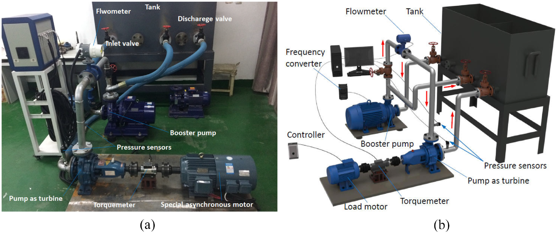
Test rig of PAT: (a) physical view and (b) model view.

The basic working process of the PAT test rig: the valves are opened, the booster pump is started and the fluid from the tank is pressurized. One part of the pressurized water flows back into the tank and the other part enters the PAT. The water passes through the PAT and then flows back into the tank. The PAT is worked by the pressurized water flow and then starts to rotate and drive the torque sensor and the frequency-controlled special three-phase asynchronous motor. The frequency-controlled three-phase asynchronous motor consumes the power generated by the PAT and controls its speed.

Pump model

Two pumps are mainly involved in this experiment, one as a booster pump and the other reversed as a PAT. The booster pump unit is a direct-connected pipeline centrifugal pump, model ISW-65-160(1). Its rated parameters are: flow rate 50 m³/h, head 32 m, speed 2900 r/min. The prototype pump for the PAT is a centrifugal clear water pump, model IS80, 50, and 200 J. Its rated parameters are: flow rate 25 m³/h, head 12.5 m, speed 1450 r/min. The diameters of the pump inlet and outlet are 80 and 50 mm, respectively. Six twisted blades are used. The inlet blade angle of the flow line in the middle of the blade is 20° and the outlet angle is 42.5°. The blade is 3.5 mm thick, the inlet diameter of the blade is 66 mm, and the outer diameter of the impeller is 202 mm. The impeller inlet is 34 mm wide and the outlet is 9.0 mm wide. The inlet width of the spiral volute is 24 mm, and the diameter of base circle of the volute is 210 mm.

Experimental scheme

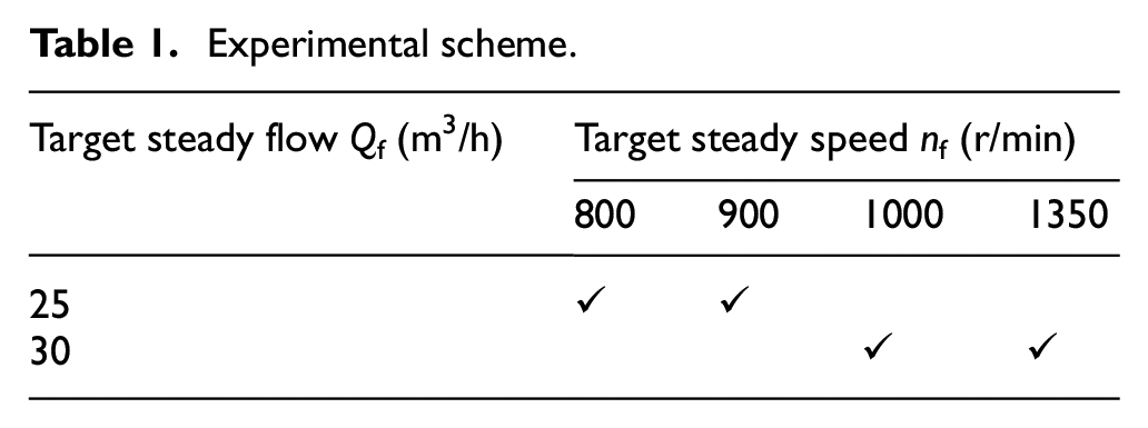
The test scheme in this paper is shown in Table 1. Firstly, after the PAT was started, two kinds of speed (800 and 900 r/min) were tested at a steady flow rate of 25 m³/h (defined as the micro- valve opening case), the former being marked as low speed (low) and the latter as high speed (high) in this flow case for easy identification. The outlet valve opening is then increased so that the steady flow rate is 30 m³/h (defined as the small valve opening case), and then the experiments are carried out at speeds of 1000 and 1350 r/min respectively, also marking the former as low (low) and the latter as high (high) for this flow rate case.

Table 1.

Experimental scheme.

Target steady flow Q_f (m³/h)	Target steady speed n_f (r/min)
Target steady flow Q_f (m³/h)	800	900	1000	1350
25	✓	✓
30			✓	✓

Results analysis

Micro-valve opening startup

Rotational speed characteristics

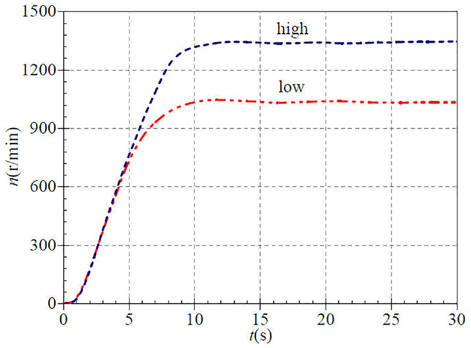
Figure 2 shows the speed variation curves of the PAT during an atypical start-up for different steady speed scenarios. The corresponding steady speeds after start-up are 800 and 900 r/min, respectively. It can be seen that the two speed rise curves have similar evolutionary characteristics in the low and high steady speed situations: at the beginning of the start-up, the two speed curves rise very slowly, then gradually speed up, and when they are close to a steady state, the rate of rise shows signs of slowing down and eventually tends to stabilize. The speed rises very slowly until about 1.2. At 1.2 s, the transient speed values corresponding to the two curves are 8.1 and 8.5 r/min respectively, with very little difference between the two curves. After 1.2 s, the rate of increase of the speed curve gradually increases. The rate of curve rise corresponding to the high steady speed slows down at about 10.2 s, slightly ahead of the slowdown at 11.8 s in the low steady speed case. At the same time, it can be seen that the rate of rise of the high speed curve is greater than that of the low speed curve during most of the start-up process. The low and high steady speed curves reach their steady values in approximately 12.9 and 14.0 s, respectively, also with the high stability speed curve slightly ahead of schedule. The final stable values of the high speed curve are higher than that of the low speed curve, with the corresponding stable values of 937.2 and 870.7 r/min, respectively. The difference between the steady speed tested and the speed expected in the scenario is probably related to the unstable voltage during the experiments.

Figure 2.

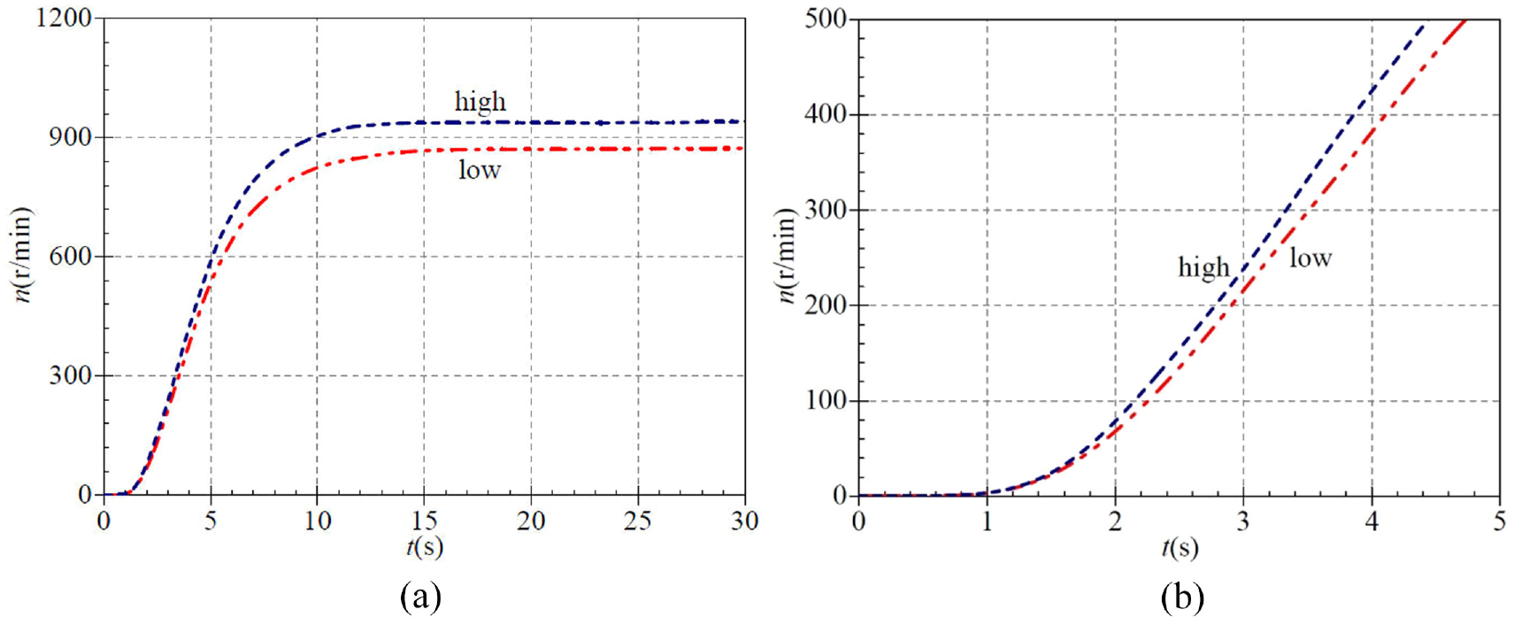
Rising characteristics of rotational speed (micro-valve opening): (a) whole and (b) part.

Flow characteristics

Under the same test conditions, the transient flow curves measured during the atypical start-up of the PAT are shown in Figure 3. In the test, the steady state flow rate of the PAT after start-up was achieved by adjusting the outlet valve opening, which is an early active adjustment, so the actual measured steady flow rate in the end differed very little from the target scheme value. The curve characteristics can be found in the graph, in the two stable speed operating conditions, the corresponding flow curve rising trend is basically the same, there are slight differences. That is, the flow rate rises very slowly at the beginning of the start-up, then the rate gradually accelerates, and eventually the curve decelerates and stabilizes. Until 1.5 s, the rate of flow rise is very small and the two curves almost coincide. At 1.5 s, the transient flow rates for the low and high steady speed cases are 0.12 and 0.134 m³/h, respectively. Then the rising rates of the two curves increase rapidly. At about 15.9 s, the transient flows corresponding to the two flow curves are 16.614 m³/h and 16.800 m³/h, respectively. After 15.9 s, the rising rate of the low-speed flow curve tends to decrease slightly. Until about 26.2 s, the low-speed flow curve reaches a relatively stable flow value, corresponding to a stable flow value of about 25.131 m³/h. The flow curve at high steady speed starts to stabilize at around 30.0 s, with a final stable value of around 25.075 m³/h. The difference between the two flow stability values is very small. It can be seen that the time required for the flow curves to reach a stable value lag significantly behind the time required for the rotational speed to be stable. Moreover, a relatively obvious flow shock occurs at high steady speeds, but it does not happen at low steady speeds. The shock occurs at approximately 25.1 s after start-up, corresponding to the maximum flow value of 25.722 m³/h and the shock flow (defined as the difference between the maximum and steady flow values) is 0.647 m³/h.

Figure 3.

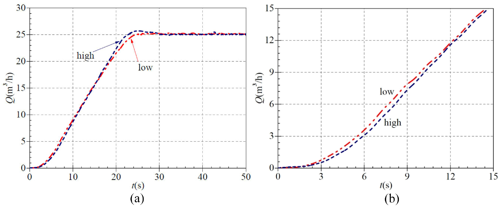
Rising characteristics of transient flowrate (micro-valve opening): (a) whole and (b) part.

Inlet and outlet static pressure characteristics

Under the same test conditions as above, the evolution of the inlet and outlet static pressures as a function of time corresponding to low and high steady speeds during the atypical startup of the PAT is shown in Figure 4.

Figure 4.

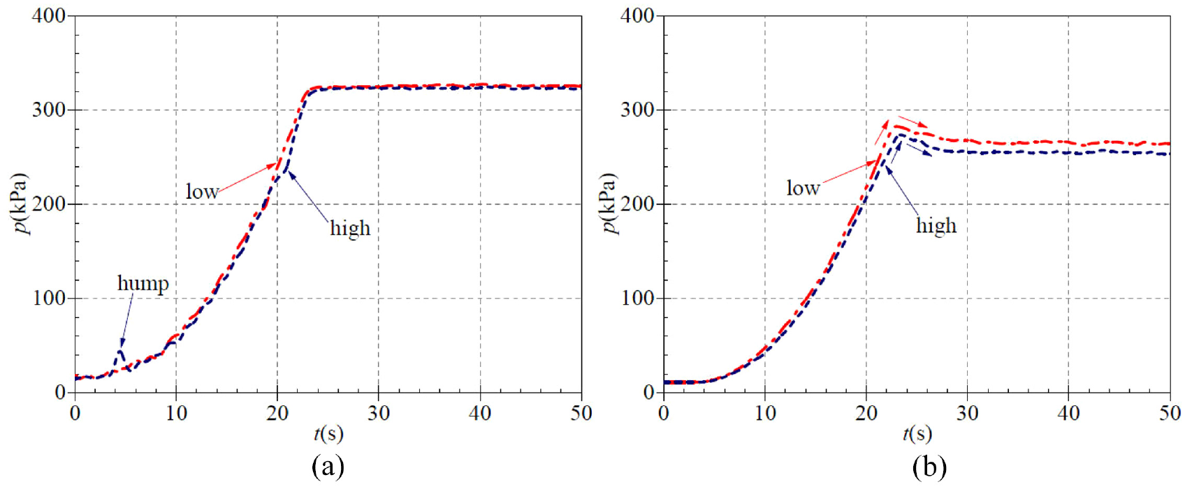
Rising characteristics of transient static pressure (micro-valve opening): (a) pump inlet and (b) pump outlet.

Figure 4(a) shows the variation curves of the inlet static pressure. It can be found that the rising characteristics of the two static pressure curves corresponding to the low and high steady speeds are approximately the same, with small differences. At the beginning of start-up, the transient static pressures corresponding to the two curves are 19.0 and 15.0 kPa, respectively. Until about 7.1 s, the rate of rise of the curves is relatively slow. At 7.1 s, the transient static pressures corresponding to the two hydrostatic curves are about 35.592 and 33.344 kPa, respectively. After 7.1 s, the rising rate of the hydrostatic curve gradually increases. Until about 24.1 s, the two curves basically reach a stable state, the corresponding stable static pressure values of the two static pressure curves are about 325.918 and 322.952 kPa, respectively. During the acceleration, the static pressure curve at high steady speed conditions shows a peak of small amplitude, which quickly returns to normal. The peak occurs at about 4.4 s and corresponds to a transient static pressure of approximately 44.248 kPa. Although the rising characteristics of the two curves are essentially similar, the static pressure value for the low-stable speed case is always slightly greater than that of the high-stable speed case for most of the time period, as is the eventual corresponding stable value. As can be seen from the graph, the degree of fluctuation during the rise of the static pressure curves at the inlet increases with the increase in speed after the start-up has stabilized.

Figure 4(b) shows the evolution of the static pressure at the outlet of the PAT as a function of time. In the case of low and high steady speed, the trend of the outlet static pressure curves is also basically similar. At the beginning of start-up, the static pressure curves of the outlet rise very slowly, and then gradually accelerate, until the two curves occur successively with small amplitude of static pressure shock phenomena, and then gradually reduce, and finally both tend to be stable. It can be seen from the figure that the transient static pressure corresponding to both curves at the beginning of the start-up process is 11.375 kPa. In the 4.9 s after the start-up, the amplitude of rise is very small, the two curves are almost the same. After 4.9 s, the rising rate increases rapidly and continues until 23.0 s, when the static pressure curve corresponding to the low steady speed appears the static pressure shock phenomenon first, which corresponds to the maximal transient static pressure value of about 283.100 kPa. The moment of shock phenomenon in the static pressure curve at the high steady speed case is about 23.4 s, which lags slightly with the former, and the corresponding maximal transient static pressure value is about 273.948 kPa. Then the two curves are gradually decelerated down to the stable values at about 33.2 and 28.8 s, corresponding to the stable static pressure values of about 264.640 and 255.792 kPa, so the shock static pressure values are about 18.460 and 18.156 kPa, respectively. The difference between the steady static pressure values at the outlet under the two steady speed cases is about 8.848 kPa. Similar to Figure 4(a), the two curves have basically similar characteristics. The static pressure value at the low steady speed case is always slightly higher than that at the high steady speed case for most of the time period. It can be seen that the static pressure value at the outlet decreases as the steady speed increases, and there is a slight lag in the occurrence of the static pressure shock and the degree of the static pressure shock is gradually decreasing.

Combined with Figure 4(a) and (b), it can be seen that the initial moment of the start, the inlet static pressure is slightly higher than the outlet static pressure, and the time to reach a stable state of the outlet static pressure curves are significantly lagged with the inlet static pressure curves. The phenomenon of static pressure shock only occurs at the outlet, not at the inlet, which is mainly due to the PAT outlet static pressure shows a certain degree of fluctuation caused by the action of dynamic and static interference. The final stable static pressure value of the inlet curve is higher than that of the outlet static pressure curve. In addition, in the same flow conditions, both in the inlet and outlet, the static pressure curve corresponding to the low steady speed is overall slightly higher than the static pressure curve corresponding to the high steady speed, that is, with the increase in the steady speed after start-up, the static pressure value will gradually decrease.

Head characteristics

During the atypical startup of the PAT, the evolution of the transient head corresponding to two different steady speeds with time is shown in Figure 5. It can be seen that the rise of the head curves significantly fluctuates compared to the changes of other external characteristics of the PAT, with peaks and valleys of relatively large amplitude. Both head curves also rise slowly at the beginning of the start-up, then the rising rate will rapidly accelerate, and finally rise to a relatively stable range of fluctuations, both have more stable average head values. The head curve corresponding to the high steady speed shows an overall rising trend with small fluctuations within about 19.1 s after start-up. During this period, a local maximal value occurs at about 4.4 s, followed by a rapid return to the normal value. The transient head value corresponding to this maximal value is about 2.89 m. The transient head value is about 2.12 m when it rises slowly to 19.1 s, and then drops rapidly to a local minimal value at about 20.9 s, with the transient head value about 0.86 m. And then at about 28.0 s, the head curve rises rapidly to a relatively stable state. After that, the high speed head curve has a small fluctuation, and the average value of the period is relatively stable, about 6.6 m. In the case of low steady speed, the head curve rises gradually at a slower rate within 17.6 s after start-up, also with small fluctuations. Local minimal values appeared at 8.3 s and 18.8 s, corresponding to the transient head values of 0.2 m and 0.5 m, respectively. Then it rises to a relatively stable state with a fast and then slow rate. At about 25.5 s, the rising rate of the head curve corresponding to the low speed tends to slow down significantly, and the corresponding transient head value is about 4.7 m at this moment. Finally, it rises to a relatively stable state at about 32.5 s, also with small fluctuations, and the corresponding average value is about 5.8 m. It can be seen that with the increase of the steady speed, the value of the steady head at the end of the start-up also increases gradually, and the moment when the head curve reaches the relative steady state is also advanced.

Figure 5.

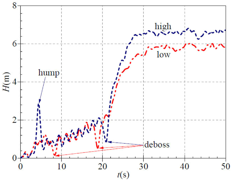
Rising characteristics of transient head (micro-valve opening).

Shaft power characteristics

Through the values of the transient speed and transient torque measured in the test, the transient shaft power of the PAT during the start-up can be calculated. As shown in Figure 6, it is a graph showing the change of the PAT shaft power under the same starting conditions. It can be seen that in the low and high steady speed cases, the rising trend of the shaft power curve is basically the same. In the first 1.2 s of start-up, the rising rate of the shaft power curves is very small and the two curves are almost identical. At 1.2 s, both curves correspond to a transient shaft power value of approximately 0.00114 kW, then rise rapidly, and finally gradually decelerate up to a relatively stable state. The two curves reach stable values at approximately 12.7and 11.7 s, with corresponding stable values of 0.124and 0.137 kW, respectively. Among them, starting from about 4.7 s, the rising rate of the shaft power curve at low steady speed first shows signs of slowing down, after which the difference between the two curves corresponding to the shaft power gradually becomes obvious.

Figure 6.

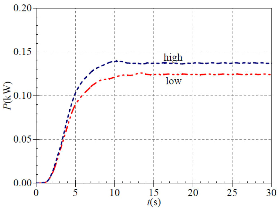
Rising characteristics of transient shaft power (micro-valve opening).

It can be seen that with the increase of the steady speed, the steady shaft power after start-up must also increase. Among them, the rising rate of the shaft power curve at high stable speed slows down a little later, but reaches a relatively stable state earlier.

Small-valve opening startup

Rotational speed characteristics

The steady flow at small valve opening is about 30 m³/h. At this opening, the speed variation curves corresponding to the low and high steady speeds of the PAT during the atypical startup are shown in Figure 7. The low and high steady rotational speeds are 1000 and 1350 r/min, respectively. By comparing the two curves in the figure, it can be seen that the trend of speed change is basically the same, both of which go through a rising process from slow to fast, then from fast to slow, finally gradually becoming stable.

Figure 7.

Rising characteristics of rotational speed (small-valve opening).

During the initial 0.8 s of startup, both curves rise very slowly. The transient speed values corresponding to the two curves at 0.8 s were almost the same, and the values were about 18.2 r/min. Then the rising rate gradually increases. Until about 5.0 s, the rising rate of the low speed curve begins to slow down, corresponding to the transient speed of about 748.8 r/min. The moment when the rate of high steady speed curve slowed down is obviously lagged, and the time point is about 8.5 s, corresponding to the transient speed of approximately 1263.7 r/min. Finally, at about 12 s after start-up, the high and low steady speed curves rise to a relatively stable state at about the same moment, corresponding to steady speed values of about 1341.7 and 1046.7 r/min, respectively. Compared with the speed curve under the micro-valve opening, it can be found that the speed under the small-valve opening tends to stabilize earlier. This is because when the valve opening is increased, the larger flow rate acts as a higher torque for the PAT impeller, so the rising rate is faster. Similarly, there is a difference between the speed in the expected scheme and the measured speed, which is also mainly due to the unstable voltage during the experiment.

Flow characteristics

As shown in Figure 8, under the startup conditions of small valve opening (stable flow of 30 m³/h), the evolution characteristics of the flow curves corresponding to the two stable speeds are generally similar, with minor differences. At the beginning of startup, the rising rate of the flow curves are both small, followed by a rapid rise, and finally the curves gradually decelerate and rise to stable values. Overall, the flow value of the low-speed curve is higher than the corresponding flow value of the high-speed curve during most of the rising process. At the beginning of the start-up, the rising rate of the low-speed curve is significantly higher than that of the high-speed curve. The rise of the high steady speed curve is very small until about 2.4 s, and the transient flow value corresponding to 2.4 s is about 1.404 m³/h. After that the rising rate increases rapidly. Until 19.1 s, the rate becomes very small, but still maintains an increasing trend. At about 28.9 s, the flow shock phenomenon occurs with a maximal flow value of about 31.588 m³/h. Then it slowly decreases again to the stable value, and the time to reach the stable value is about 35.9 s, and the stable flow value is about 30.047 m³/h, corresponding to the shock flow value of about 1.541 m³/h. In the low steady speed case, the rising rate of the flow curve is small before 0.9 s, and the difference with the high speed curve is small. However, from 0.9 s, the rising rate of the low-speed flow curve increases rapidly, which is earlier than that of the high-speed curve, and the transient flow value corresponding to the low-speed curve is about 0.482 m³/h at this moment. Then it goes through a fast to slow rising process until it reaches a relatively stable state at about 20.4 s, and the corresponding transient flow rate is about 30.273 m³/h, without any obvious flow impact phenomenon.

Figure 8.

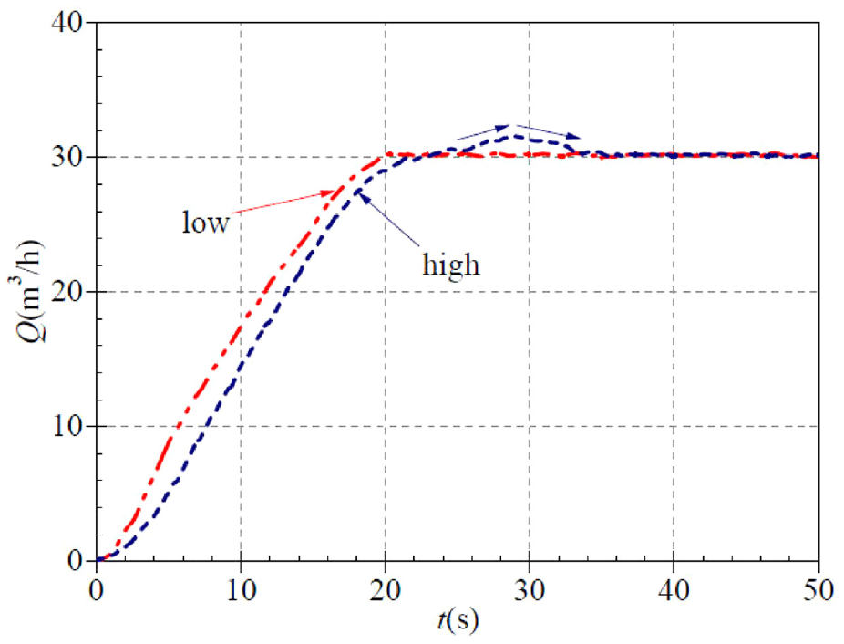
Rising characteristics of transient flowrate (small-valve opening).

Similarly, the steady flow in the test is also regulated by the outlet valve opening. Therefore, there is little difference between the flow value after startup stabilization and the scheme preset flow value. It can be seen that the situation is similar to that of the micro-valve opening. Under the same flow conditions, the flow shock phenomenon is more obvious at higher steady speeds.

Inlet and outlet static pressure characteristics

During the small valve opening startup, different steady speeds are set, and the variation of the static pressure curves measured for the PAT inlet and outlet are shown in Figure 9(a) and (b). Among them, Figure 9(a) shows the variation characteristics of the static pressure at the PAT inlet, and it can be seen that the variation trends of the two static pressure curves are similar overall, with small differences. At the beginning, the static pressure value at the inlet of both curves is 14.0 kPa. In the initial 1.3 s of startup, the static pressure curve rises slowly at the high steady speed. The transient static pressure value at 1.3 s is approximately 15.306 kPa, and then the rate of rise increases rapidly. At about 2.4 s, there is a relatively obvious peak, which falls rapidly again and returns to the normal rate of rise. In this paper, the startup of pump as turbine belongs to the atypical startup, namely that the pump startup works on fluid medium, meanwhile the fluid medium derives the pump as turbine to start. Therefore, the static pressure at inlet of pump as turbine in Figure 9(a) actually reflects the evolution characteristics of the static pressure at the outlet of the booster pump during atypical startup process. The peak phenomenon occurred present experiments is also observed in existing article.²¹ The reason for peak phenomenon may be attributed that the fluid medium in the whole circulatory system is stationary before atypical startup. When the booster pump start, which would generate a abrupt impact on the stationary fluid body. The transient static pressure value corresponding to the peak is about 53.098 kPa. Then the curve rises at a high rate, reaching a steady state at about 21.2 s with a steady value of about 303.905 kPa. Similarly, the static pressure curve corresponding to the low steady speed rises less before 4.0 s. The transient static pressure value at 4.0 s is approximately 25.349 kPa. Then the curve rises rapidly until it reaches a stable value at about 20.9 s, corresponding to the stable value of about 303.968 kPa. The stable static pressure values are almost identical for both curves. It can be seen that the fluctuation in the rise of the static pressure curve is more obvious at high steady speeds, even with a relatively obvious peak appears in the early startup phase.

Figure 9.

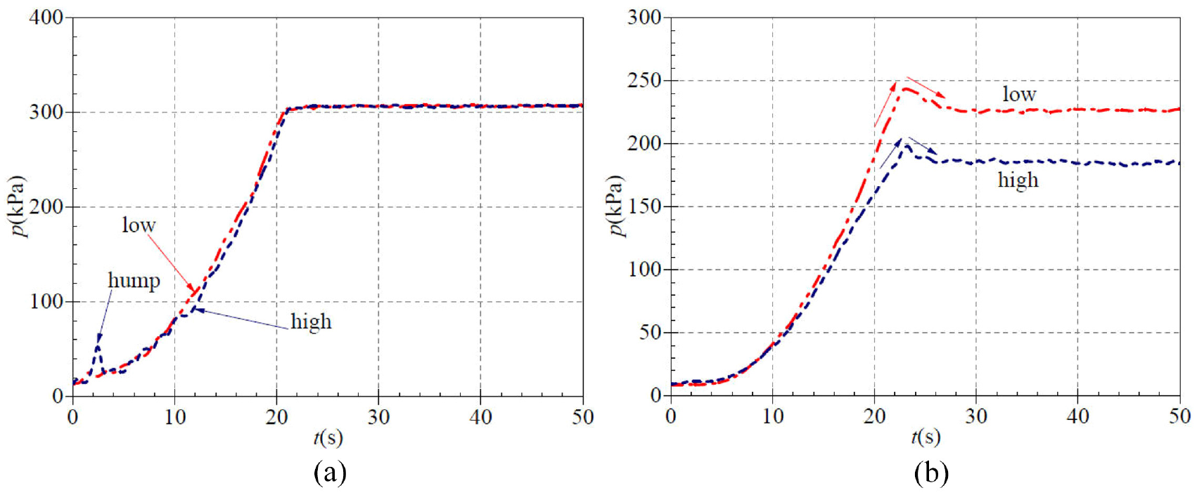
Rising characteristics of transient static pressure (small-valve opening): (a) Pump inlet and (b) Pump outlet.

Figure 9(b) shows the variation curves of the static pressure at the outlet of the PAT. The rising trend of both curves is also nearly similar. The static pressure values at the initial moments are 8.938 and 9.50 kPa for the low and high steady speed cases respectively. For the first 4.0 s, both static pressure curves rise very slowly, with transient static pressure values of 9.610 and 11.781 kPa at 4.0 s, respectively. Then the two curves rise rapidly, reaching the maximal value at about 23.1, 23.2 s, respectively, and the phenomenon of static pressure shock appears. The maximal transient static pressure values are 243.482 and 198.256 kPa, respectively. Finally the two curves reach stability at approximately 28.0 and 26.0 s, corresponding to the values of 227.005 and 185.309 kPa, respectively. Therefore, the static pressure shock values (the difference between the maximum and the stable static pressure value) are 16.477 and 12.947 kPa, respectively. The difference between the stable static pressure values is approximately 41.696 kPa. It can be seen that, with the increase of the steady speed after the startup process, the static pressure value of the outlet will gradually decrease, and the phenomenon of static pressure shock shows a trend of gradually lagging and weakening.

Combining (a) and (b) in Figure 9, it can be seen that at the initial moment of startup, the static pressure values at the inlet of the PAT are higher than those at the outlet. The time for the static pressure at the outlet to rise to a steady state is slightly delayed compared to the inlet, After the PAT has started to stabilize, the values of the static pressure at the inlet are higher than the values at the outlet. In comparison with the data for the micro-valve opening case, the increase in the steady flow and speed values after start-up reduces the static pressure values at both the turbine inlet and outlet. No matter what the valve opening or steady speed conditions, the phenomenon of static pressure shock only occurs at the outlet of the PAT. This means that during the atypical startup of the PAT, static pressure shocks are prevalent at the outlet of the PAT. It is also due to the PAT outlet static pressure shows a certain degree of fluctuation caused by the action of dynamic and static interference. In terms of the time nodes at which the curve characteristics occur, the differences between the two static pressure curves at the same operating conditions are not significant. In addition, in the same flow condition, with the increase of the steady speed, the fluctuation of the static pressure value curve at the inlet becomes more dramatic. It can be found that the curves corresponding to the two high steady speeds at the inlet appear obvious local maximal values under different flow conditions. And the static pressure stable value at the outlet also shows a gradually decreasing trend with the increase of the stable speed, and the degree of static pressure shock will also be reduced to some extent.

Head characteristics

As shown in Figure 10, the head evolution curves corresponding to different steady speeds during the startup of the PAT with small valve opening. It can be seen that during the rise, both head curves are accompanied by small fluctuations, but it is obvious that the curve fluctuations are more dramatic at high steady speed. Both curves show a more obvious head shock phenomenon before stabilization. Then, the two curves decrease rapidly, with local minimal values, and finally rise gradually and tend to be stable. At the beginning of the start-up period, about 2.4 s, the head curve in the case of high steady speed appears a local maximal value, and then quickly returns to a more normal rate of rise. The transient head value at 2.4 s is about 3.80 m, while the low speed curve does not show any obvious sudden change in the process of rise. Subsequently, the two curves gradually accelerate upward, and the head shock phenomena occur in different degrees successively. The curves at the low and high steady speeds reach their maximal values at 20.3 and 21.1 s, corresponding to the transient head values of 9.22 m and 12.71 m, respectively. Then, both curves go through the evolution process of first decreasing and then increasing and finally tending to be stable. At about 23.5 s and 23.1 s, the two curves drop to local minima, and the corresponding transient head values are 5.78 m and 10.55 m. Finally, the two curves gradually rise again to relatively stable states, corresponding to time points of about 27.8 and 26.0 s, and the stable transient head values are 7.68 and 11.91 m, respectively. The shock heads corresponding to the two curves are 1.54 and 0.80 m, respectively. And the differences between the respective steady values and local minima are 1.90 and 1.36 m. It can be seen that under the same flow condition, the degree of head shock and the difference between the stable value and the local minima decrease gradually with the increase of the stable speed, and the head shock phenomena occur slightly earlier.

Figure 10.

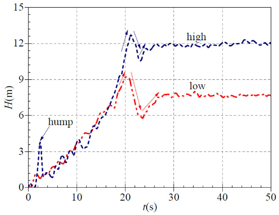
Rising characteristics of transient head (small-valve opening).

Compared with the startup process under the micro-valve opening shown in Figure 5, it can be found that after the steady flow increases to a certain extent, there will be relatively obvious head shock phenomena. At the same time, the time required for the PAT head to reach the relative steady state will be slightly advanced with the increase of the steady flow. Under the same flow condition, the steady head after starting gradually rises with the increase of the steady speed. The degree of fluctuation of the rising head curve is also more obvious, but the time for the head curve to reach the steady state will be advanced.

Shaft power characteristics

By setting the stable flow and speed conditions, combined with the measured experimental data, it is possible to calculate the shaft power of the PAT in the atypical startup process. And the variation trend of shaft power is shown in Figure 11. From the figure, it can be found that the two curves have a similar rising trend, both of which experience a slow rise, then a rapid rise, and then a gradual deceleration and stabilization, similar to the case of the micro-valve opening. In the initial stage of about 0.6 s, the rise of both shaft power curves is very small. The difference between the two curves is very slight. And both transient shaft power values are about 0.00177 kW at this moment. Then both curves enter a fast rising stage, until the two curves reach the relatively stable state. The shaft power curve at the high steady speed situation suddenly becomes stable at about 7.8 s. And the rising trend from high speed suddenly turns smooth and stable. The deceleration time is very short, and the stable value is about 0.238 kW. While the curve at the low steady speed gradually decelerated at 5.2 s, the transient shaft power value was about 0.173 kW. Until it reaches the steady state at about 8.7 s, the corresponding steady shaft power value is about 0.206 kW. It can be seen that the rising rate of the low-speed curve is slightly faster than the high-speed curve in the first part of the rising process. But the deceleration is more obvious in the latter part of the time period, and the deceleration phenomenon appears in advance.

Figure 11.

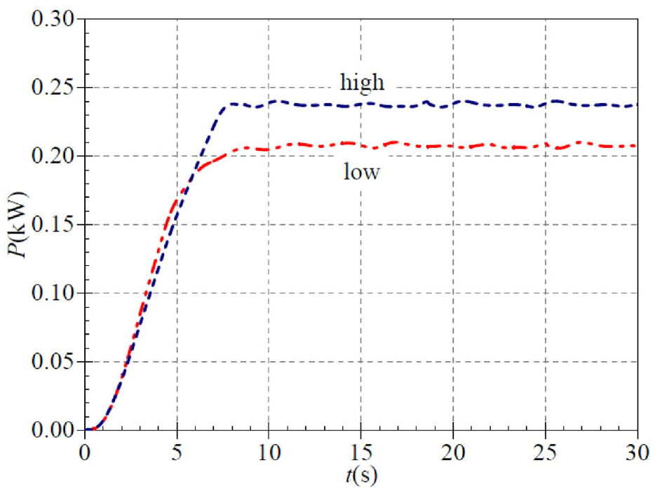
Rising characteristics of transient shaft power (small-valve opening).

Combining Figures 6 and 11, it can be found that under the same flow condition, the shaft power inevitably increases with the increase of the steady speed. Also the moment of starting the deceleration phenomenon is slightly delayed, but the time required to reach the steady state is advanced. With the increase of steady flow and steady speed, the time required for the shaft power to be stable decreases.

Dimensionless analysis

The atypical startup process is described in terms of the dimensionless volumetric flowrate, the dimensionless head, and the dimensionless shaft power as a function of time. The three are defined as follows.

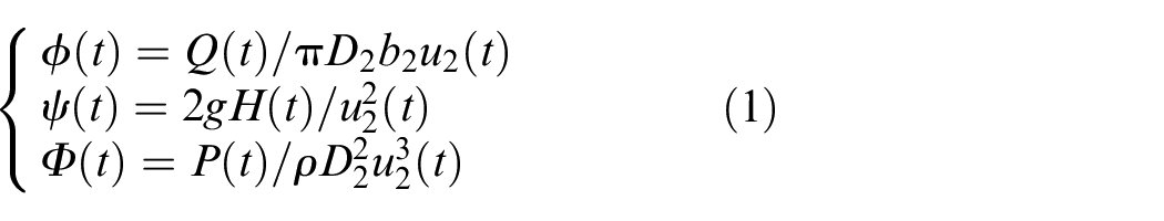
{\begin{matrix} ϕ (t) = Q (t) / π D_{2} b_{2} u_{2} (t) \\ ψ (t) = 2 gH (t) / u_{2}^{2} (t) \\ Φ (t) = P (t) / ρ D_{2}^{2} u_{2}^{3} (t) \end{matrix}

(1)

Among these, $u_{2} (t)$ is the transient circumferential velocity at the impeller outlet, the expression of which is $u_{2} (t) = π D_{2} n (t) / 60$ . The evolutions of transient dimensionless flow, dimensionless head and dimensionless shaft power with time during atypical start-up are given in Figures 12 to 14, respectively.

Figure 12.

Rising characteristics of dimensionless flowrate: (a) micro-valve opening and (b) small-valve opening.

Figure 13.

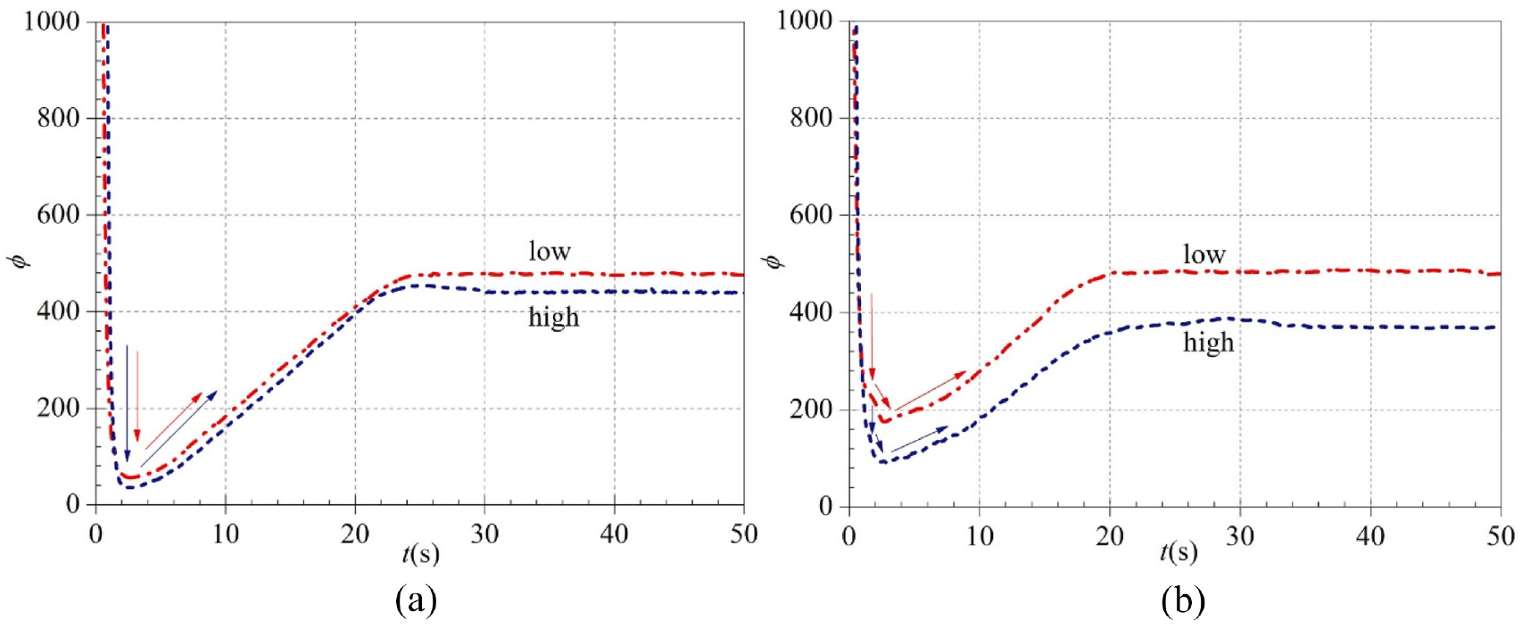
Rising characteristics of dimensionless head: (a) micro-valve opening and (b) small-valve opening.

Figure 14.

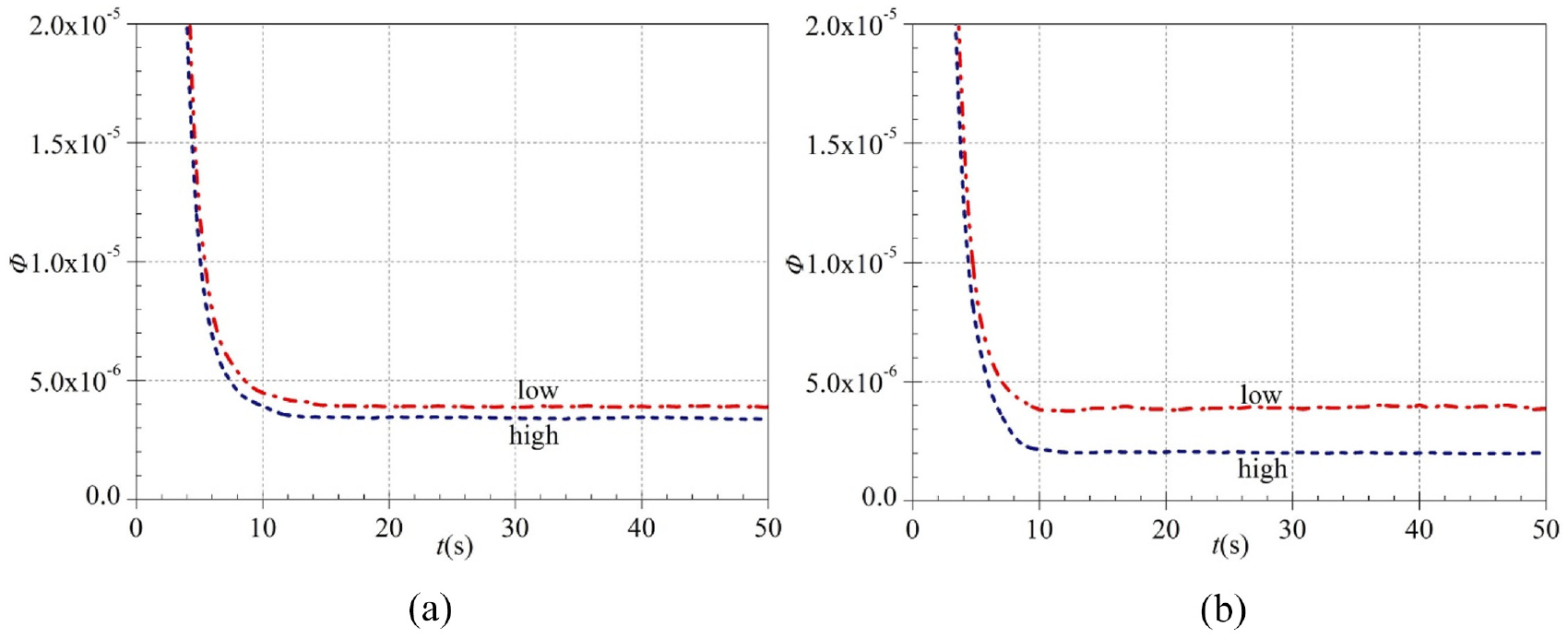
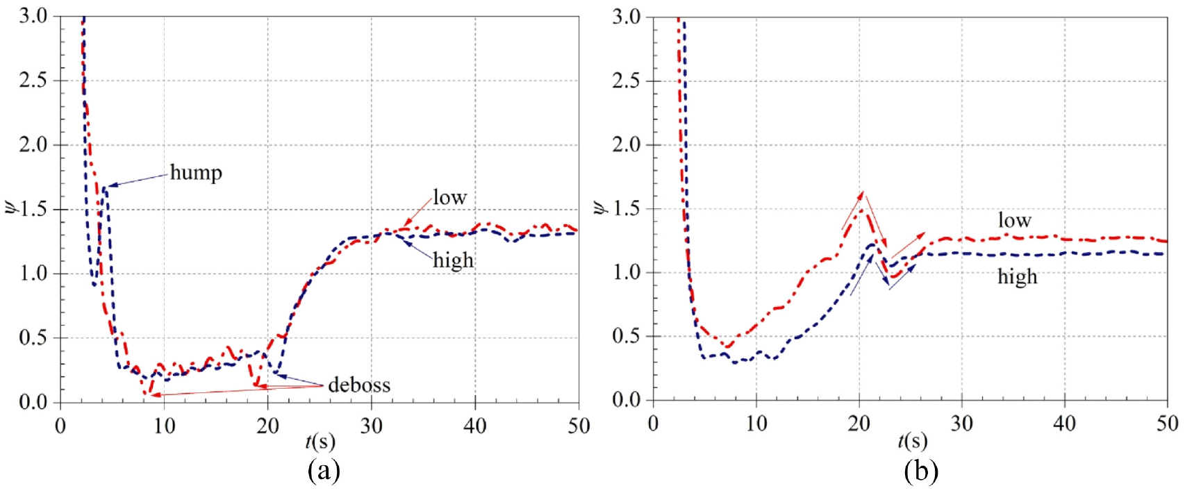
Rising characteristics of dimensionless shaft power: (a) micro-valve opening and (b) Small-valve opening.

Dimensionless flowrate

An atypical startup test of the PAT is conducted by setting two different sets of steady speeds at each of the two valve openings. Combined with the above definition, the trends of the resulting dimensionless flow factor with time are shown in Figure 12. It can be seen that the variation trends of the dimensionless flow factors corresponding to different steady speeds are generally similar under the two valve openings. That is, all the dimensionless flow factors have a very large value at the initial moment of startup, then drop to a minimum value extremely fast, followed by a gradual upward trend. Finally, the curves all reach relatively stable states. However, the minimum value to which each dimensionless flow factor curve drops to, as well as the value and time point at which each curve reaches a stable value, also vary under different start-up conditions.

The variation curves of the dimensionless flow factors corresponding to different steady speeds at micro valve openings (25 m³/h) are shown in Figure 12(a). The low and high steady speeds are 800 and 900 r/min, respectively. It can be seen that the time taken to drop from the extremely large values at the beginning of start-up to the minimum values are approximately 2.7 and 2.4 s, respectively, corresponding to minimum values of about 56.250 and 35.896, respectively. At the high steady speed, the dimensionless flow factor curve shows a very small amplitude shock at approximately 25.1 s, with a transient maximum value of about 453.671, followed by a slow decline to a steady value. Eventually the curves of the dimensionless factors all reach stable values. And the time to reach the stable value is 25.1 and 30.1 s, respectively, corresponding to the stable values of 476.385 and 439.292. Therefore, the shock difference in the high stable case is about 14.379. It can be seen that under the micro-valve opening condition, the steady value of the dimensionless flow factor tends to decrease gradually with the increase of the steady speed instead, and the time to reach the steady state is delayed.

Figure 12(b) shows the variation curves of the dimensionless flow factors for different steady rotational speeds at small valve openings (30 m³/h). The steady speed conditions corresponding to the two curves are 1000 and 1350 r/min, respectively. As can be seen from the figure, there are maximal values for both curves at the beginning of the startup, and then rapidly fall to minimum values, which take about 2.6 and 2.9 s, respectively. The minimum dimensionless flow factors are about 175.329 and 90.632, respectively. Although the decline in the curve is very rapid, it is clear that the rate of decline, compared to the initial rate, diminishes to some extent at about 1.2 s. This is more evident at the steady speed of 1000 r/min. The transient dimensionless flow factors of the two curves at 1.2 s are 246.362 and 186.490, respectively. As the two curves fall to their minimum values, they begin to rise again gradually. Among them, the curve corresponding to the high steady speed shows a small amplitude shock phenomenon at about 28.9 s and then gradually decreases toward stabilization, with the transient value at 28.9 s about 388.542. The time for the two curves to reach steady state is 21.4 and 34.0 s, respectively, and the corresponding steady values for the dimensionless flow coefficient are 479.966 and 368.717. The shock value of the dimensionless flow factor at the high steady speed is approximately 19.825. It can be observed that the increase in steady speed for small valve opening conditions delays the time to reach the steady value of the dimensionless flow factor. And the final steady value tends to decrease.

Combining Figure 12(a) and (b) with the definition of the dimensionless flow factor, it can be seen that both flow and rotational speed are important factors in determining the variation characteristics of the dimensionless flow factor. The high steady speed in Figure 12(a) is 900 r/min and the low speed in Figure 12(b) is 1000 r/min. With the increase of the steady flow, the steady value of the dimensionless flow factor at the higher steady speed also increases. Therefore, with the increase of the steady flow, the dimensionless flow factor also shows an increasing trend. For the two valve openings, the respective dimensionless flow curves for the high steady speed case show very small shocks. In addition, the variation of the dimensionless flow factor curves during the gradual ramp-up is very similar to the flow curve, with highly coincident time points. This is mainly due to the fact that the time points at which the rotational speed tends to stabilize are significantly earlier, when the flow and head curves show characteristic phenomena, the rotational speeds are largely stable or have changed very little.

Dimensionless head factor

Figure 13 shows that the trends in the dimensionless head coefficient curves are somewhat similar under the two steady flow conditions and the different steady speeds. At the beginning of startup, no matter what kind of stable flow and speed conditions, all curves have maximal values, then drop rapidly, and then rise gradually after maintaining a relatively stable level for a while. Eventually all the curves reach more stable states than before. Compared with the other two dimensionless coefficients, the fluctuations in the rising curves of the dimensionless head coefficient are the most dramatic.

Among them, Figure 13(a) shows the micro valve opening case. The two curves correspond to steady speeds of 800 and 900 r/min after start-up. The values of the dimensionless head factor are very large at the beginning of start-up and then drop to lower levels at an extremely fast rate. During the rapid decline, the curve corresponding to the high steady speed will appear a local maximum, and then decrease rapidly. The time when the local maximum occurs is about 4.2 s, which corresponds to a transient dimensionless head factor of 1.679. The similar phenomenon does not occur in the low steady speed case. During the period of maintaining the low levels, two and one minima occur in the low-speed and high-speed curves, respectively. The 2 time points when the minimum values appear in the low steady speed case are 8.4 and 18.8 s. And the corresponding transient dimensionless head factor values are about 0.056 and 0.138. The time when the very small value appears in the high stable speed case is about 20.7 s, with the transient value of about 0.232. Then all the curves gradually rise back up. Until about 27.8 s, the high stable speed curve reaches a relatively stable state first, with a stable value of about 1.274. While the low stable speed curve rises to the stable value at about 31.3 s, corresponding to a stable value of about 1.347. It can be noticed that during the curve rebound, the low speed curve shows an early deceleration, but the high speed curve reaches a steady state early. Although the differences in the final steady values are small, the dimensionless head factor is always slightly higher in the low speed steady case.

Figure 13(b) shows the evolution of the dimensionless head factor curves of the pump as a turbine over time during the small valve opening startup process. The two curves correspond to stable speeds of 1000 and 1350 r/min at the end of the startup process, both of which also have maximal values at the beginning of the startup and then drop to very low levels at an extreme rate. After the gradual rebound of both curves, there are relatively significant shocks. After the gradual rebound of both curves, there are relatively significant shocks. Then the curves drop below the stable level and eventually rise again to relatively stable states. The shock occurs at 20.3 and 21.3 s, corresponding to transient dimensionless head values of 1.484 and 1.217, respectively. Then the two curves drop to local minima at about 23.5 and 23.1 s, corresponding to transient values of 0.971 and 1.051, respectively. During the rebound process, the high steady speed curve reaches the steady level first, at about 26.0 s, corresponding to the steady value of about 1.147. While the low steady speed curve lags slightly, reaching its steady value at about 27.8 s, and the steady value is about 1.253. The shock values corresponding to the dimensionless head at low and high speeds are 0.231 and 0.07, and the difference between the stable and local minima is 0.282 and 0.096, respectively. It can be found that at small valve openings, with the increase of the steady speed, the shock degree of the dimensionless head factor tends to lag and weaken significantly. As well as the difference between the steady value and the local minimal value decreases gradually.

In combination with Figure 13(a) and (b), it can be seen that the variation in the dimensionless head curve corresponding to the lower steady speed is more dramatic at the same steady flow condition. With the increase of the steady speed, the dimensionless head curve reaches the steady state earlier, and the steady state value decreases slightly. In comparison, it can be seen that with the increase in steady flow, the minimum value of dimensionless head increases and the time point from the minimum value rises significantly earlier. It also leads to stronger fluctuations in the dimensionless head curve before it reaches a steady state. This causes a certain degree of shock too, which is more noticeable at the low steady speed. In addition, during the rebound of the dimensionless head factor curves, the time points when the local minima and shocks occur are highly coincident with the time points when the corresponding head curves show similar phenomena. The same reasons as for the dimensionless flow factor curves are mainly due to the fact that the speed tends to stabilize at significantly earlier points in time. When the characteristic phenomena of the flow and head curves appear, the speed is almost stable or the changes are already small.

Dimensionless shaft power

During the atypical startup, the trends of the dimensionless shaft power coefficient curves for the PAT are shown in Figure 14. As can be seen from the figure, the trend of the dimensionless shaft power curves is essentially the same even at different valve openings and different steady speed cases. At the beginning of the start-up, all curves have maximal values, which then drop at an extremely fast rate and then gradually decelerate down to a stable value, eventually maintaining very stable states.

Figure 14(a) shows that the startup of the PAT is carried out at a micro valve opening (25 m³/h), with the low and high steady speeds of 800 and 900 r/min, respectively. At the beginning of the start-up, both curves fall rapidly from extremely large values. At about 8.0 s, the decreasing speed of both curves gradually slows down until they reach their respective steady states. The corresponding transient dimensionless shaft power values are about 5.371 × 10⁻⁶ and 4.565 × 10⁻⁶, respectively. Finally, both curves reach relative steady states at about 12.0 s, corresponding to stable values of 3.891 × 10⁻⁶ and 3.432 × 10⁻⁶ for the dimensionless shaft power at the end of start-up.

Figure 14(b) shows the variation curves of the dimensionless shaft power factor during the start-up of the PAT at a small valve opening (30 m³/h). The corresponding steady speeds after start-up are 1000 and 1350 r/min, respectively. Similar to the situation in Figure 14(a), both curves fall rapidly from the initial maximal values at start-up, and then gradually decelerate to steady states. The decreasing rate begins to diminish gradually at about 8.0 s. The transient dimensionless shaft power factors at this point are about 4.426 × 10⁻⁶ and 2.705 × 10⁻⁶, respectively. Then, at about 10.7 s, both curves reach stable values, which correspond to the stable values of 3.786 × 10⁻⁶ and 2.123 × 10⁻⁶, respectively.

It can be seen that under the same flow conditions, the decreasing rate of the dimensionless shaft power factor curves tends to increase slightly with the increase of the steady speed. While the final corresponding steady value decreases gradually. Combining Figure 14(a) and (b), it can be seen that the high steady speed of 900 r/min in Figure 14(a) and the low steady speed of 1000 r/min in Figure 14(b), which correspond to stable values of the dimensionless flow factor of about 3.432 × 10⁻⁶ and 3.786 × 10⁻⁶, respectively. It can be seen that the stable value of the dimensionless shaft power factor increases with the increase of the stable flow value.

Discussion

Under the micro-valve opening (25 m³/h) and small-valve opening (30 m³/h), two groups, that is, Four different low and high steady speeds (800, 900, 1000, and 1350 r/min) are set up respectively. The transient hydraulic performances of the pump as a turbine during the atypical start-up are investigated. It can be seen that only two steady speeds are set for each set of steady flow conditions, the conclusions that can be observed are rather limited. Therefore, in the next related work, more reasonable experimental protocols will be set up to fully and systematically investigate the influence of speed and flow rate on the transient characteristics of the PAT during atypical startups. Meanwhile, it is seen that the flow shock phenomenon occur under the condition of high-speed startup, while no shock phenomenon occur when low-speed startup. Therefore, the threshold for not occurring needs to be deeply studied in the near future.

Conclusions

In the same flowrate, the flow shock phenomenon generally occurs in the case of a high stable speed. The increase in stable flowrate leads to the emergence of the head shock phenomenon. The increase in rotational speed leads to the gradual reduction in the degree of head shock. The flowrate, head, dimensionless flow and head curves are significantly delayed from the rotational speed curves. All three dimensionless factors curves have maximal values at the beginning of the startup period. Both the dimensionless flowrate and head curves generally show a rapid decline from maximal values to lower levels and then a gradual increase to relatively stable levels. The dimensionless shaft power factor curves decrease directly and rapidly from maximum values to stable values.

Footnotes

Author contributions

Yu-Liang Zhang carried out experiments and analyzed the characteristics of PAT; Kai-Yuan Zhang wrote the manuscript, Jin-Fu Li and Jun-Jian Xiao checked the manuscript and revised it. All authors have read and agreed to the published version of the manuscript.

Declaration of conflicting interests

The author(s) declared no potential conflicts of interest with respect to the research, authorship, and/or publication of this article.

Funding

The author(s) disclosed receipt of the following financial support for the research, authorship, and/or publication of this article: The research was financially supported by the National Natural Science Foundation of China (Grant No. 51876103), “Pioneer” and “Leading Goose” R&D Program of Zhejiang (Grant No. 2022C03170) and Zhejiang Provincial Natural Science Foundation of China (Grant No. LZY21E060001).

ORCID iD

Yu-Liang Zhang

Data accessibility

The data used to support the findings of this study are available from the corresponding author upon request.

References

Kitteredge

Thomas

. Centrifugal pumps operated under abnormal conditions. J Power Sources 1931; 73: 881–884.

Fecarotta

McNabola

. Optimal location of pump as turbines (PATs) in water distribution networks to recover energy and reduce leakage. Water Resour Manag 2017; 31: 5043–5059.

Frosina

Buono

Senatore

. A performance prediction method for pumps as turbines (PAT) using a computational fluid dynamics (CFD) Modeling Approach. Energies 2017; 10: 103.

Doshi

Channiwala

Singh

. Inlet impeller rounding in pumps as turbines: an experimental study to investigate the relative effects of blade and shroud rounding. Exp Therm Fluid Sci 2017; 82: 333–348.

Derakhshan

Kasaeian

. Optimization, numerical, and experimental study of a propeller pump as turbine. J Energy Resour Technol 2014; 136(1): 7.

Singh

Nestmann

. Internal hydraulic analysis of impeller rounding in centrifugal pumps as turbines. Exp Therm Fluid Sci 2011; 35: 121–134.

Jain

Swarnkar

Motwani

, et al. Effects of impeller diameter and rotational speed on performance of pump running in turbine mode. Energy Convers Manag 2015; 89: 808–824.

Barbarelli

Amelio

Florio

. Predictive model estimating the performances of centrifugal pumps used as turbines. Energy J 2016; 107: 103–121.

Santolaria Morros

Fernández Oro

Argüelles Díaz

. Numerical modelling and flow analysis of a centrifugal pump running as a turbine: unsteady flow structures and its effects on the global performance. Int J Numer Methods Fluids 2011; 65: 542–562.

10.

Maleki

Ghorani

Haghighi

MHS

, et al. Numerical study on the effect of viscosity on a multistage pump running in reverse mode. Renew Energy 2020; 150: 234–254.

11.

Abazariyan

Rafee

Derakhshan

. Experimental study of viscosity effects on a pump as turbine performance. Renew Energy 2018; 127: 539–547.

12.

Yang

S-S

Derakhshan

Kong

F-Y

. Theoretical, numerical and experimental prediction of pump as turbine performance. Renew Energy 2012; 48: 507–513.

13.

Yang

S-S

Kong

F-Y

X-Y

, et al. Influence of blade number on the performance and pressure pulsations in a pump used as a turbine. J Fluid Eng 2012; 134(12): 23.

14.

Wang

Kong

Xia

, et al. The method for determining blade inlet angle of special impeller using in turbine mode of centrifugal pump as turbine. Renew Energy 2017; 109: 518–528.

15.

Miao

Yang

Shi

, et al. Research on energy conversion characteristic of pump as turbine. Adv Mech Eng 2018; 10: 168781401877083.

16.

Sen-Chun

Hong-Biao

Ting-Ting

, et al. Optimal design of blade in pump as turbine based on multidisciplinary feasible method. Sci Prog 2020; 103: 36850420982105.

17.

Qian

Wang

Guo

, et al. Performance evaluation of an axial-flow pump with adjustable guide vanes in turbine mode. Renew Energy 2016; 99: 1146–1152.

18.

Lin

Zhu

, et al. Investigation of flow separation characteristics in a pump as turbines impeller under the best efficiency point condition. J Fluid Eng 2021; 143: 061204.

19.

W-G

. Effects of viscosity on turbine mode performance and flow of a low specific speed centrifugal pump. Appl Math Model 2016; 40: 904–926.

20.

W-G

. Optimising prediction model of centrifugal pump as turbine with viscosity effects. Appl Math Model 2017; 41: 375–398.

21.

Zhang

Y-L

Zhu

Z-C

W-G

. Experiments on transient performance of a low specific speed centrifugal pump with open impeller. Proc IMech Eng, Part A: Journal of Power and Energy 2016; 230: 648–659.

Effect of rotational speed and flowrate on the startup characteristics of a pumps as turbine

Abstract

Keywords

Introduction

Test rig and experimental mode

Test rig

Pump model

Experimental scheme

Results analysis

Micro-valve opening startup

Rotational speed characteristics

Flow characteristics

Inlet and outlet static pressure characteristics

Head characteristics

Shaft power characteristics

Small-valve opening startup

Rotational speed characteristics

Flow characteristics

Inlet and outlet static pressure characteristics

Head characteristics

Shaft power characteristics

Dimensionless analysis

Dimensionless flowrate

Dimensionless head factor

Dimensionless shaft power

Discussion

Conclusions

Footnotes

Author contributions

Declaration of conflicting interests

Funding

ORCID iD

Data accessibility

References