Sage Journals: Discover world-class research

Abstract

In this work, the authors aim at developing a reliable and fast methodology to evaluate the wear evolution in tire starting from a complete optical 3D scanning. Starting from a data cloud, a semi-automatic methodology was implemented in MATLAB to extract mean tread radial profiles in correspondence of the desired angular position of the tire. These profiles could be numerically evaluated to establish the presence of irregular wear and the characteristic parameter of the groove depth. The reliability and the robustness of this methodology was firstly tested by applying it to several synthetic case studies modeled in CATIA V5^®, where ovalization and presence of defects were also simulated. The groove depth was determined with an error lower than 1% for the ideal model, while the introduction of ovalization and defects leaded to an error of 2.6% in the worst condition. In a second time, the methodology has been successfully applied to experimental measurements carried out in two different wear life of the tire, allowing the tracking of the wear phenomena through the evaluation of the progressive lowering of tread radial profiles.

Keywords

3D scanning tire wear evaluation discrete models tread profile

Introduction

When two bodies are in relative motion, the friction between the contact surfaces causes the wear of the surfaces themselves. The wear can be defined as a loss of material that modifies the surface profile affecting the performance of a component. The study of wear is a very important challenge in the tribology field since its quantitative evaluation is essential for the research advance for improving wear resistance and service-life. The analysis of surfaces focused on the wear monitoring allows identifying profiles that are optimized to achieve higher performance and durability, without neglecting the advantage to reduce manufacturing, maintenance, and replacement costs.

Wear phenomena involved in the contact of tire and asphalt pavement is particularly relevant in the automotive sector. Wear tire is responsible of the decay of the vehicle performance, both in terms of safety and efficiency. On the other side, the degradation of asphalt pavement determines the increase of noise and vibration, a reduction of the comfort for the passenger and in general a lack of safety condition associated to mobility. Another important aspect to be considered is that the wear interesting tire and asphalt is a relevant source of PM10 particles, especially in an urban context. Consequently, the development of tools that allow studying the wear phenomena constitutes an important challenge for the transport sector.

The different nature of tire and asphalt leads to different statistical approaches to describe the wear phenomena, which are evidently more complex in the case of the asphalt pavement.^1,2 However, in all cases the possibility to reconstruct the effective geometry of the surfaces using 3D laser scanners give the possibility to reach a more accurate description and to provide advanced tools for the study of the wear.

Limiting the attention to the case of tire, several digital methods are available to carry out tire wear evaluation, as reported briefly in Akkök et al.³ The main methods have been identified in Stachowiak et al.⁴ and resumed in the following:

- Weighing⁵: the difference in the weight before and after the use allows quantifying the material loss in the component.

- Ultrasonic reflectometry and phase interference^6,7: these methods can be used to evaluate with high resolution the thickness reduction due to the wear.

- 2D digital image processing^8–12: geometry modification of the component is evaluated through a quantitative analysis of binary images, after appropriate pre-processing and segmentation operations.

- optical microscopy, 2Dprofilometry: these methods require the use of optical non-contact profilometers and microscopes. They are very accurate, simple, and fast.¹³

- 3D scanning: acquisition of 3D geometry of surfaces and reconstruction of the whole component.¹⁴

These last methods are very interesting for the considered case, since they are based on non-contact measurements. At this purpose, the absence of contact allows avoiding the error introduced by the pressure exerted by measurement tool on the high deformable surface of tire.

The approach that allows following the wear phenomena in all its complexity and that provides results based on the largest amount of data is based on the acquisition of the 3D geometry of the involved surfaces. Therefore, it represents a necessary tool to provide a quantitative basis for the reconstruction of the phenomenon and the validation of new models and procedures.¹⁵

In the case of a tire, driving safety and ride comfort are affected by its progressive wear that also influences the maneuverability, hydroplaning, fuel consumption, and noise generation.¹⁶ Since the wear modifies the tread pattern structure influencing the tire performance, it is a not-negligible phenomenon in a scenario where the vehicle performance is an urgent challenge in the competition among tire companies. The top and bottom surface and grooves are the principal features of the tire pattern configuration and strongly influence the tire performance and quality. For this reason, the wear status evaluation is important to preserve the tire functions. The depth of the tread groove is a crucial factor influencing the braking performance of the vehicle and must be periodically inspected to ensure driving safety. Furthermore, its periodic evaluation at pre-fixed range of mileage represents the simplest tool for the direct analysis of the tire tread wear status and an indicator useful to follow its evolution during driving cycles. However, the evaluation of tread groove is not satisfactory if the aim is to obtain data for developing an appropriate wear model of the tire. In this case, more advanced techniques must be used.

However, it is very difficult to assess the surface topography of an object with a complex surface morphology as a tire.¹⁶ Deep grooves, kerfs, and thin features are usually present, determining accessibility problems during the acquisition process. In order to overcome these difficulties, the last approaches reported in technical literature about the digital reconstruction of the tire surface^17,18 limited their attention to a reduced set of data, consisting in a certain number of profiles equally distributed along the circumferential direction. The choice of considering a reduced set of data allowed a simplification of the problem but had the direct consequence that the localization of the tire axis needs to be fixed a priori with the rotating axis of the experimental setup. These limitations could lead to unacceptable systematic errors in the evaluation of tire surface, especially when the same tire surface is compared at different amount of wear.

In this perspective, the aim of this study is to establish a reliable methodology able to evaluate and analyze the different stages of wear process for a tire. The surface is experimentally acquired by a non-contact measurement technique, which performs the 3D scanning of the tire surface during different stages of its life.

In comparison with the cited approaches, the novelty of the methodology here proposed is characterized by several innovations that allow a better knowledge of the surface tire topology and its comparison after driving cycles. The first innovation is represented by the fact that the evolution of the wear phenomena of tire tread is based on a complete reconstruction of the tire geometry. Consequently, the complete data set that is obtained allows to consider not only the geometrical variation of the wear having axisymmetric distribution, but also geometrical irregularities that could be randomly disposed along the circumferential direction. This limitation is easily overcame exploiting the knowledge of the whole tire surface: the proposed algorithm, in fact, allows extracting circumferential section of the tire surface that are used to identify the actual center; subsequently, the centers of this circumferential features are interpolated to determine the actual revolution axis of the tire, improving the quality of the wear evaluation.

Finally, a semi-automatic methodology has been implemented in MATLAB^® in order to extract, from tread profile, the specific parameters that are useful for tire wear evaluation. The methodology, in fact, is driven by the active choice of the user that interactively can select the position and the angular sector to be considered for the data elaboration, the specific parameters to be extracted, the specific point to be used to calculate the depth groove. This choice allows achieving the largest flexibility for the user and overcoming the difficulties that could be found in relation to the wide variety of the commercial tire pattern.

In particular, it is possible to extract a mean profile of the tire over an angular sector of the tire and determining the standard measurements of this mean profile as for example depth groove. This depth can be measured by processing suitably the tread radial profile extracted from the point cloud experimentally acquired.

After having illustrated the experimental set up for 3D acquisition of the tread surface and the implemented methodology for data processing, the work is focused on the validation of this methodology. The algorithm was firstly tested on a discrete model of tire generated synthetically into CATIA V5^®, where ovalization and presence of defects were also simulated. The tracking of wear phenomena was performed by comparing the groove depths measured from profiles extracted from “new” and “worn” tire.

Finally, a real case study was also considered using data obtained by a 3D reconstruction of a real tire mounted on a commercial car. Two acquisitions of the tread surface were performed before and after a mileage of approximately 5000 km. The methodology showed a good degree of reliability and robustness for both synthetic and experimental case studies, confirming the validity of the proposed approach.

Tire geometry and wear evaluation

The tire is the contact element of the vehicle with the road. Its task is to transfer to the vehicle the forces deriving from its interaction with the ground and to absorb part of the roughness encountered during the motion. The principal functions of a tire are reported in the following:

- the adherence to the ground;

- the deformability needed to envelop small obstacles and to absorb road irregularities to guarantee passenger comfort, the integrity of the vehicle over time and the continuity of contact with the ground;

- the resistance to penetration of accidental bodies;

- the ability to absorb the minimum energy possible during its motion (minimum rolling resistance) to maximize mechanical performance.

Tires that are normally used on the road and that are essentially mounted on passengers’ vehicles are geometrically characterized in various ways by grooves, which develop along circumferential and transverse paths: these channels, several millimeters deep, drain the water present on the road and allow cooling by convection. In particular cases, they can be made in such a way as to favor advancement on snow, mud, earth, sand, and incoherent land in general. The set of these channels forms the tread pattern and divides the tread into blocks.

An excessive or irregular wear of the tire surface, for which a simple measurement of depth tire tread is sufficient in most cases, is useful to identify and to correct several mounting or in-service errors, as for example incorrect inflation pressure, incorrect convergence of the vehicle, lose or worn parts, driving conditions, excessive load, etc. before the tire is irreparably compromised. Several examples are reported in Figure 1.

Figure 1.

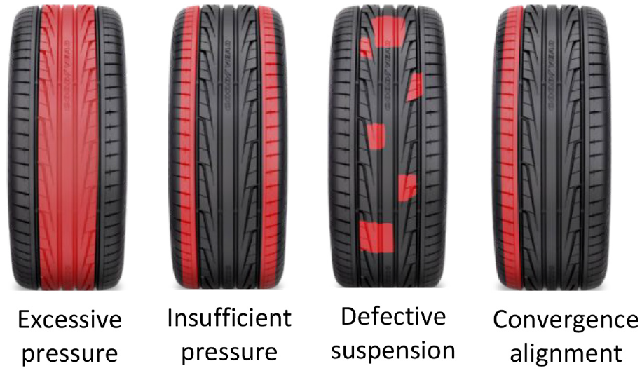
Typical wear states.

The main methods, currently used for measuring tire wear, are classified into qualitative and quantitative. The first are the following:

- the method based on the Tread Wear Indicator (TWI): most treads on the market are characterized by the presence of a small rubber insert, 1.6 mm high, placed on the bottom of the grooves. If the dowel is present, the tire bears on its side the abbreviation TWI or a small brand logo. If the tread is worn to the point of reaching the indicator, the tread thickness is no longer suitable, and the tire must be replaced (Figure 2(a));

- the coin method: the depth of the tread grooves is compared with a common coin, simply by inserting it in one of the grooves. Depending on the part of the coin that remains uncovered, the tread thickness will be suitable or not (Figure 2(b)).

Figure 2.

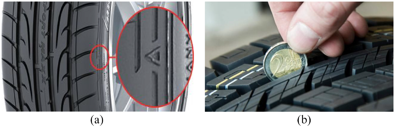
Manual methods for wear measurement: (a) tread wear indicator and (b) coin method.

Qualitative methods are commonly used during periodic maintenance to control the effective state of the tire.

To investigate tire wear thoroughly, a quantitative assessment of wear phenomena is required. Even the simplest quantitative methods measure the groove depth to monitor tire wear. These techniques are divided into two large families: contact techniques and non-contact techniques.

The most common contact technique is based on the use of a depth gage. The measurement is carried out, with the stopped vehicle, positioning the base of the caliper on two adjacent ribs and manually acting on the mobile rod until the probe enters into contact with the bottom of the groove. In most of the instruments, the digital measurement is preferred to the analog 1. Several problems are originated using the depth gage:

the alignment between the base of the gage and the ribs may not be appropriate, especially in the area near the side of the tire.

the compression of the rubber under the probe may not be uniform, modifying the measured values.

the quantitative evaluation of the tread wear requires that the measurement of the groove depth is always carried out in the same position after the various driving cycles. Using a manual measuring tool, the measurement of the groove depth is random.

the measure obtained is an average value calculated on the heights of two adjacent ribs. The tire, however, could exhibit uneven wear, with the height of one rib more consumed than the adjacent one.

The same inconveniences characterize also all the techniques based on a direct contact on the surface, as contact microscopy and profilometry using calipers, comparators, coordinated measuring machines (CMM).^19–24

Non-contact measurement techniques, on the contrary, are mainly based on the use of two methodologies: laser and structured light. The disadvantages typical of contact methods, such as for example the rubber compression, the faulty alignment of the instrument, the influence of the human factor, are completely overcome by using non-contact techniques, so obtaining more precise and accurate measurement values.²⁵ However, optical or non-contact methods are techniques applicable if direct access to the worn surface is possible.

In the recent years, the imaging-based scanners are more largely used for Reverse Engineering than Coordinate Measuring Machines (CMM) since they allow extracting high density point clouds in a very short time (over 30,000 points per second). Among the 3D scanners, those with structured light project the white light onto the object surface as a sinusoidal fringe pattern and reconstruct the curvature surface exploiting the Moiré effect.

The laser scanning technique is based on the principle of triangulation. This methodology requires that a laser beam is projected onto the object. The reflected radiation is then captured by a camera equipped with a CCD (Charge Coupled Devices) solid state sensor, to detect the position set at a predetermined distance from the laser source. Repeating this measurement following a regular scan, a point cloud is obtained. The result is a very high number of three-dimensional coordinates acquired from the surface of the scanned object (point cloud). A disadvantage common to all triangulation-based techniques is the limited applicability in all those cases in which the surfaces present sudden variations in depth (grooves, fissures, sudden changes of slope). Currently, laser scanning systems are often used to detect the profile of a tire and to evaluate its wear status: they operate in an almost completely automatic way and can acquire a very large number of points per second, offering ever better accuracy. An example of methodology using the laser scanning technique for tire wear evaluation can be found in Wang et al.,¹⁷ where the reconstruction of the tire is limited to some tread portions.

Structured light systems operate in a similar way to laser systems being much more inexpensive and faster. They exploit the same principles of triangulation, replacing the laser source with a projector of white light. To avoid the problem of relying on the variation of the texture in the object to be scanned, the system projects on the surface some specific patterns (structured encodings). If the relative position of light source and camera is known, using the principles of triangulation, it is possible to retrieve information on the geometry of the scanned object (Figure 3).²⁶

Figure 3.

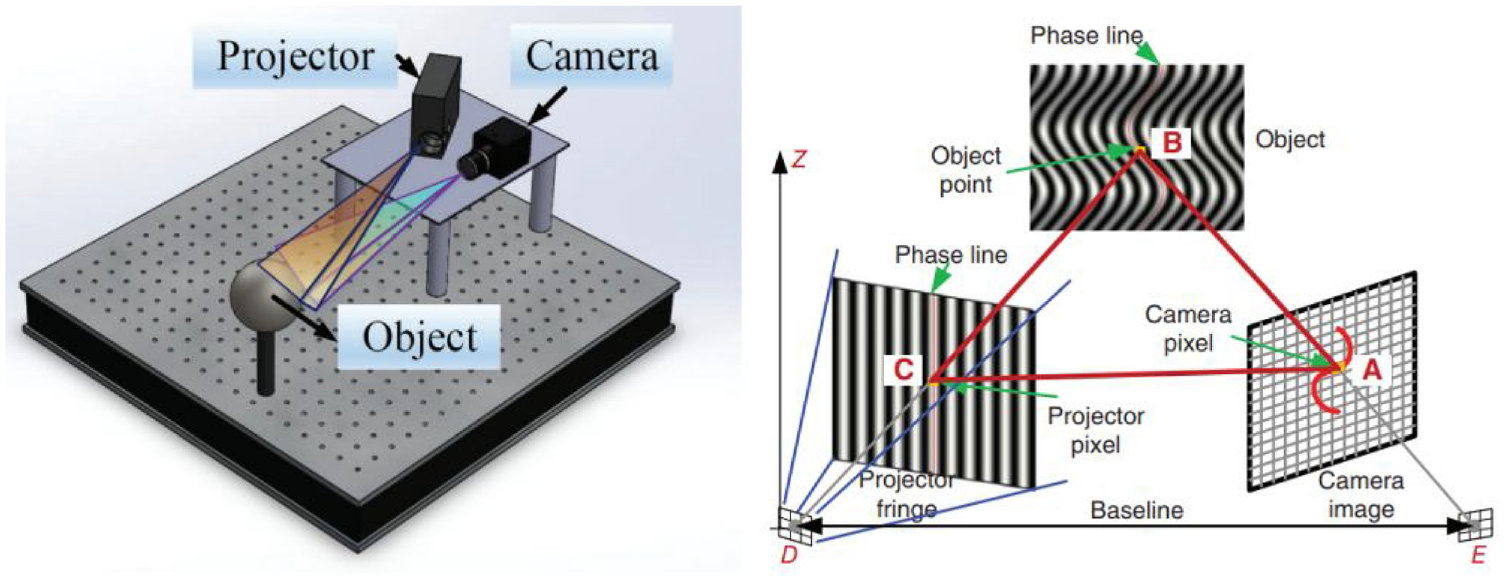
Structured light systems.²⁶

The light patterns are substantially formed by appropriately coded strips (or bands) of light. The simplest coding is carried out by assigning a different brightness to each projection direction, for example, projecting a linear intensity scale or assigning a different coloring according to the projection directions. However, due to its robustness, the coding that is mostly implemented is the so-called space-time coding of the projection directions. This coding system provides for the projection, according to a given time sequence, of n-band light patterns, suitably generated by a projector controlled by the computer. An n-bit code is thus associated with each projection direction, in which the i-th bit indicates whether the corresponding band, of the j-th pattern, is in light or not. This method allows distinguishing 2n different projection directions. The assignment of a bit to the different bands of light passes from the calculation of a suitable threshold value. This value is calculated as the average between the level of gray in the image of the fully illuminated scene and the level of gray in the image of the unlit scene. In this way, the technique becomes less dependent on the environmental lighting conditions and on the variation of the reflection properties of the object. Moreover, the calculation of the threshold value is useful for identifying the areas of shadow present in the scene, or those areas observed by the camera but not illuminated by the projector. They are characterized by the fact that they have minimal variations in the level of gray between the illuminated and the non-illuminated image. In these areas, the bands are not binarized and consequently the depth values cannot be measured. Once the n images of the striped patterns, projected onto the surface of the object, are converted into binary form, each pixel stores the n bit code that encodes the direction of illumination of the thinnest strip that illuminated it.^27,28 Knowing the geometry of the system, the direction of the optical beam of the camera and the equation of the plane of the corresponding band, the 3D coordinates of the point can be calculated by intersecting the optical ray with the plane. The structured light technique allows obtaining acquisition rate rather remarkable and an acceptable quality of reconstruction of 3D geometry for many industrial applications. Of course, the type of structured model projected onto the scene or the object to be captured plays a key role in determining the speed, the achievable resolution, and the accuracy of the system. This technology has been widely used for its reliability and practicality also in the measurement of the tread depth of a tire, providing more than satisfactory results.¹⁸ Used device allows to acquire the tire profile and it consists of an array of laser sources and several image sensors set in a linear arrangement. The limit of this system is that it does not involve automatic recognition of the tire grooves necessary for automatic measurement.

The structured light technique has been selected here to obtain the point cloud acquisition from tire tread used to verify the reliability of the proposed methodology.

The methodology for tread wear evaluation

The methodology, proposed here, is aimed at evaluating the evolution of tire’s wear stat through the measurement of the groove depth starting from the point clouds acquired during the 3D scanning of the tread. With this aim, a semi-automatic methodology was developed and illustrated by the block-diagram in Figure 4. Using a cylindrical reference system having the main axis coincident with the tire axis, the measurement of the groove depth is performed on the radial profile extracted from the tread surface. The profile is uniquely identified by specifying the angular position of the radial plane (i.e. containing the axis of the tire), by which the tread surface is cut.

Figure 4.

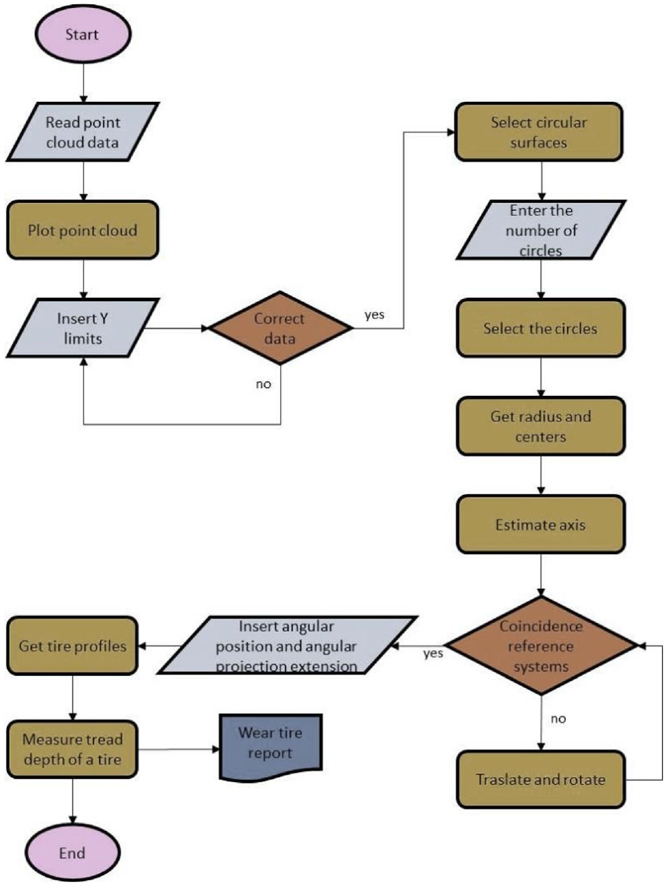
Block-diagram of the proposed algorithm.

The first step of the methodology is to estimate the tire axis, that is, the axis z of the cylindrical system. The axis, particularly, is evaluated using a linear regression model that approximates the centers of a set of circumferences suitably extracted by the axially symmetric surface of the tire.

Generally, due to grooves and tessellations, the surface of the tire tread is globally non-axial symmetric so that several axially symmetric portions must be identified to evaluate the tire axis.

Furthermore, the geometry of these surfaces must remain unchanged during driving cycles. In other words, the surfaces from which the circumferences will be extracted must not be subject to wear phenomena and therefore cannot be in direct contact with the asphalt. Figure 5 shows the bottom surfaces of the axial symmetrical grooves selected for the evaluation of the axis in the case of the tire considered here as a synthetic case study. The number and the localization of the surfaces used to extract the circumferences for the evaluation of the tire axis can be varied according to the specific pattern of the tire. However, the best choice for a better evaluation of the axis will consider a consistent number of equally spaced circumferences over the tire width.

Figure 5.

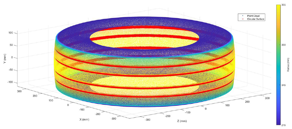
In red the bottom surfaces of the axial symmetrical grooves selected for the evaluation of the axis in the case of the tire considered as a synthetic case study.

These surfaces, since they are not in direct contact with the asphalt, should not be subjected to wear during the driving cycles and their geometry should remain unaltered. The implemented algorithm allows the user to directly select the number of areas of interest and then enter, for each of them, the y coordinates of the points that define the extension of the area of interest. For example, supposing to want to select a single circular surface, it will be sufficient to insert in the algorithm the number of circular surfaces of interest (1 in this case) and define its extension by entering the y coordinates of the limit points (Figure 6).

Figure 6.

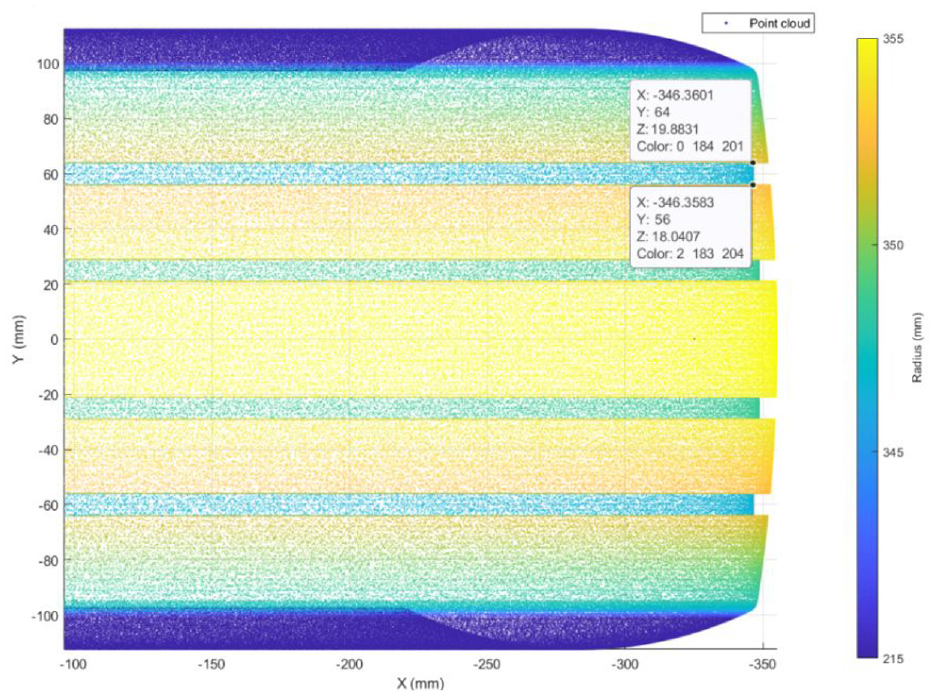
Selection of the surface of interest.

The circumferences, the number of which is defined by the user, will be automatically extracted from these surfaces at uniform distance identified by limit points (Figure 7). Obviously, the greater the number of circumferences, the greater the number of available centers for axis identification.

Figure 7.

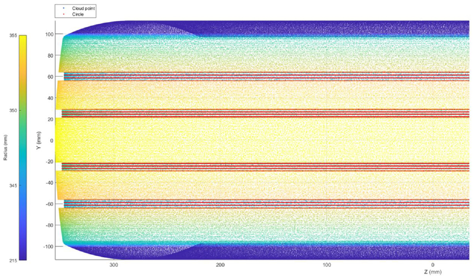
In red the circumferences extracted from the bottom surfaces of the selected grooves.

Center coordinates (a, b) and radius (R) of each circumference are evaluated through the Taubin algebraic algorithm and the Levenberg-Marquardt geometric algorithm.^29,30 The algebraic algorithm is used to provide an initial estimation to the geometric algorithm.

Taubin’s direct fitting method is an effective, nearly unbiased direct method for quadric fitting.

Recall that the Kasa³⁰ method, Taubin minimizes the following function²⁹:

F_{1} = \sum_{i = 1}^{n} {d_{i}}^{2} {(d_{i} + 2 R)}^{2}

(1)

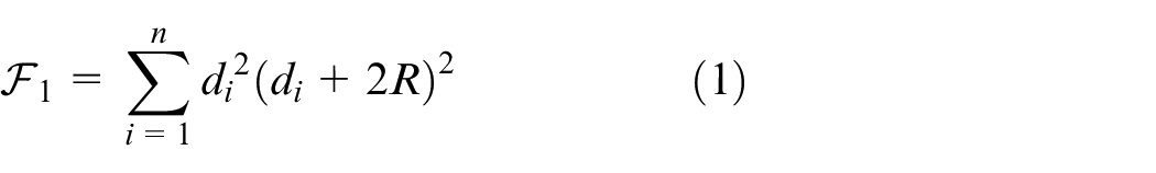
where the d_i denote the distances from the data points to the coordinates of the circle (a; b; R). Assuming the natural assumption $| d_{i} | ≪ R$ , it can derive the approximation:

F_{1} \approx 4 R^{2} \sum_{i = 1}^{n} {d_{i}}^{2}

(2)

Now the same assumption $| d_{i} | ≪ R$ can be used as follows:

R^{2} \approx {(d_{i} + R)}^{2} = {(x_{i} - a)}^{2} + {(y_{i} - b)}^{2}

(3)

Furthermore, it can improve this approximation by averaging:

R^{2} \approx \frac{1}{n} \sum_{i = 1}^{n} {(x_{i} - a)}^{2} + {(y_{i} - b)}^{2}

(4)

Finally, the linear regression on the centers of the circumferences suitably extracted provides the axis equation.

This approach could be of difficult implementation in the cases in which the tire pattern does not present circumferential features, as for example for tires that are mounted on industrial and agricultural vehicles. In this case, the algorithm will extract a certain number of circumferential arcs, depending on the specific tire pattern, and the Taubin algorithm will be applied to an uncomplete circumferential data set without problems.

Once the tire axis is known, it is possible to define a cylindrical coordinate system with axis z coincident with the axis of the tire. The introduction of this reference system is essential for correctly identifying the tread radial profiles on which the measurement of the tread depth will be performed. For a given radial profile of the tire tread, the trend of wear phenomena over the driving cycles can be tracked.

There are various ways to extract the tread radial profiles from the tire.

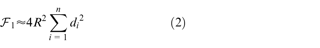
A first mode used here is to subdivide, the point cloud acquired from the entire tread into a few circular sectors angularly equally spaced. For a given value of the angular opening β the number of circular sectors n, which is considered, is equal to

n = \frac{360 °}{β}

(5)

For each sector, the radial profile is extracted by projecting the relative points on the center plane. The evaluation of the wear phenomena will be more or less accurate depending on whether this angle is more or less wide.

A second mode consists of directly setting the angular extension β and the angular position α of the relative center plane of one or more circular sectors (Figure 8). In this case, only the portion of the point cloud, which falls within the circular sector specified, will be analyzed. In this case, the 3D scanning of the tire tread can be limited to the portions of interest for wear evaluation. In this way, the algorithm can complete the analysis in less time than in the first mode, providing the user with precise information on the state of wear of the tire.

Figure 8.

Circular sector selection.

Once the tire profiles have been extracted (Figure 9), it is possible to assess the state of wear after a driving cycle, through the measurement of the groove depth.

Figure 9.

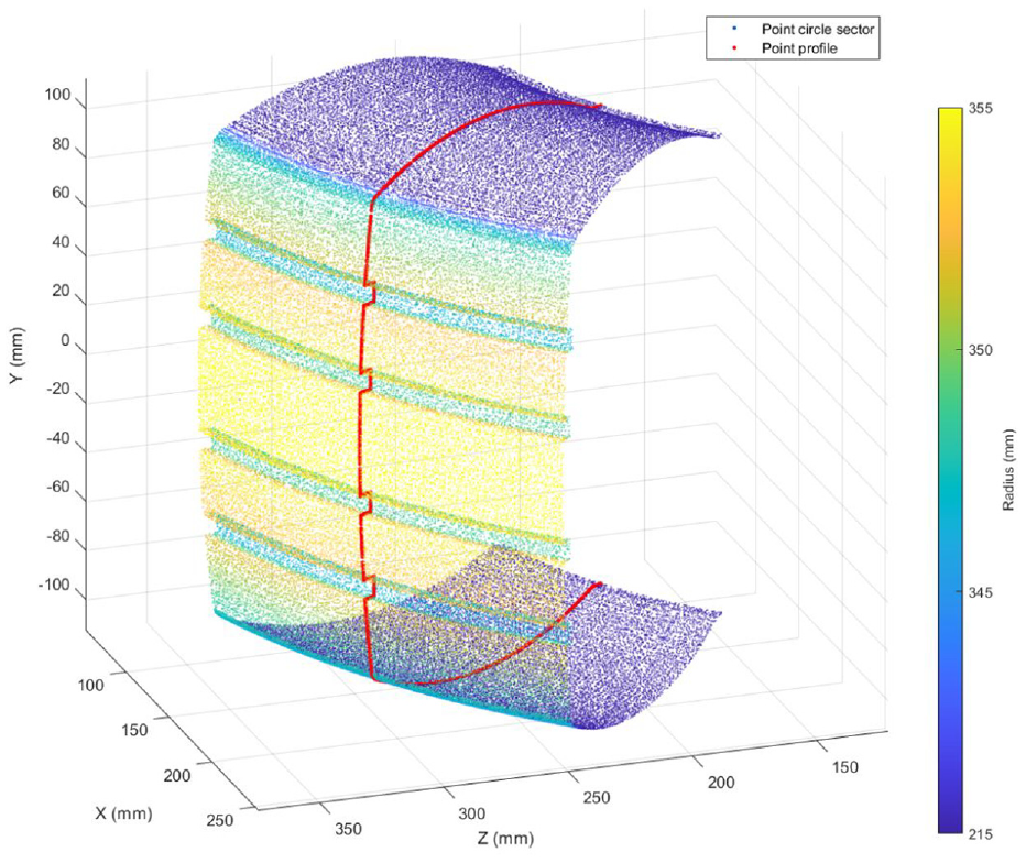
In red, the obtained profile.

The measurement of the groove depth (Figure 10) can be performed interactively or automatically. In the interactive mode, the depth is calculated as difference between the coordinates of two points selected respectively on the external surface of the tread and on the bottom surface of the groove.

Figure 10.

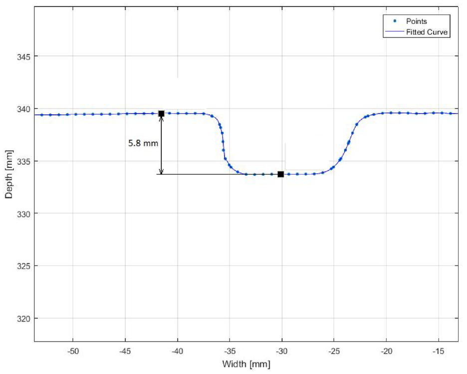
Grooves depth evaluation.

The automatic measurement of the groove depth needs the recognition of the grooves which is based on the geometric properties that characterize the profile of the tread:

- the curvature in the profile changes suddenly when passing from the straight lines, that are the vertical lines, which delimit the groove, and the horizontal ones that correspond to the bottom surface;

- on the bottom surface, the ordinate of the center of curvature is larger than the ordinate of the specific point of the profile, with respect to which the curvature is calculated;

- the width of the grooves is less than the distance that separates one groove from the next. Figure 11 clarifies this procedure.

Figure 11.

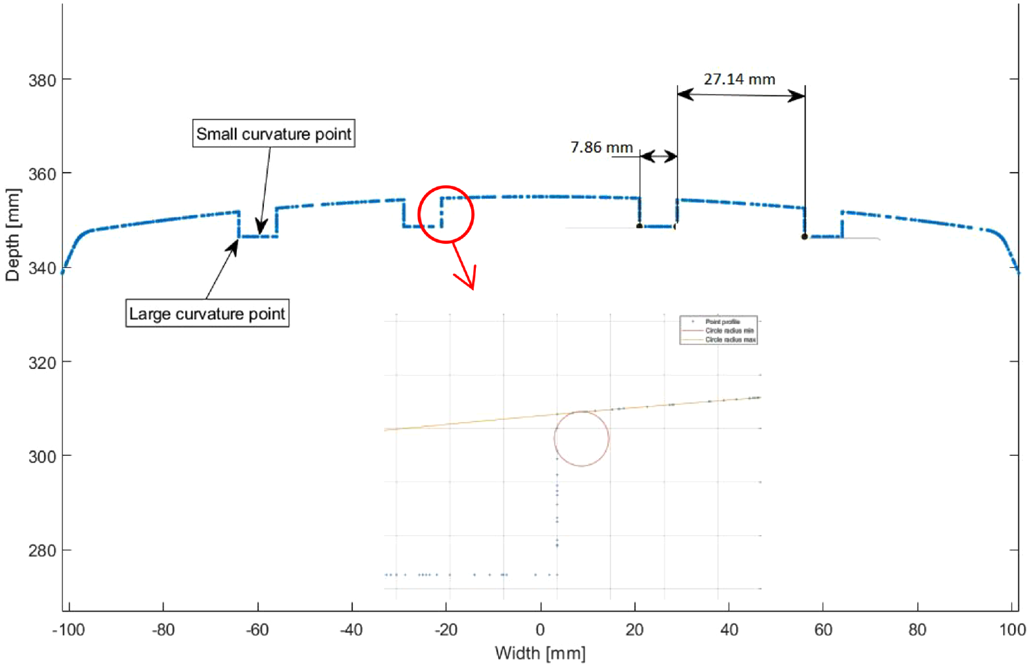
Automatic identification of the grooves.

The curvature evaluation is carried out on all the points of the radial profile, except for the tire shoulder, which is not subject to wear.

For this purpose, a sliding “control window” is used. This window must include a set of q points (with q > 3), sufficient to estimate the radius r and center of curvature of the least-squared circle approximating these points. The curvature, evaluated as 1/r, will be assigned to the center point of the sliding window.

The groove depth is measured as the difference between the average radius of the points belonging to the external surface of the tread and that of the points belonging to the bottom surface of the grooves (top flat surface, bottom flat surface).

In cases of tire pattern that does not present circumferential features, the absolute values of the groove depth cannot be easily defined and measured, but the knowledge of the axis will allow the evaluation of the wear measuring the difference between the tire profiles before and after a driving cycle.

The evolution of the tire wear status will be evaluated by tracking the reduction of the groove depth over the driving cycles.

To evaluate the lowering of the tread thickness, the methodology, once automatically segmented the points on the external surface of the tread and on the bottom surface, approximates them through polynomial functions. The groove depth will be measured after each driving cycle (Figure 12).

Figure 12.

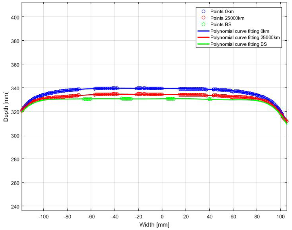
Tread depth evolution.

Preliminary tests

In order to test and validate the methodology, a 3D CAD model of a generic tire with an axial symmetric pattern has been generated into CATIA V5^®. The model is characterized by the presence of four grooves having a depth of 6 mm. This simple geometry is characterized by an ideal geometry, since it has been generated using a commercial CAD with numerical truncation errors that are at least two orders of magnitude lower of the real tire. Therefore, the cloud point obtained starting from the 3D model has been considered as an ideal geometry and indicated as ideal tire in the following considerations.

In a second time, this model has been changed introducing several geometrical irregularities and defects, to verify the capability of the methodology to capture these geometrical particularities. The first defective model is indicated as defective tire and has been obtained including spheres having 3 and 5 mm of diameter in correspondence of the second groove to alter the axial symmetry of the tire and consists of inclusions. The second defective model is indicated as wear tire and consists of a uniform circumferential wear of the tire, which determine a reduction of the groove depth.

The details of the tests and the corresponding results are reported in the following for the different cases.

Case 1: Ideal and not worn tire

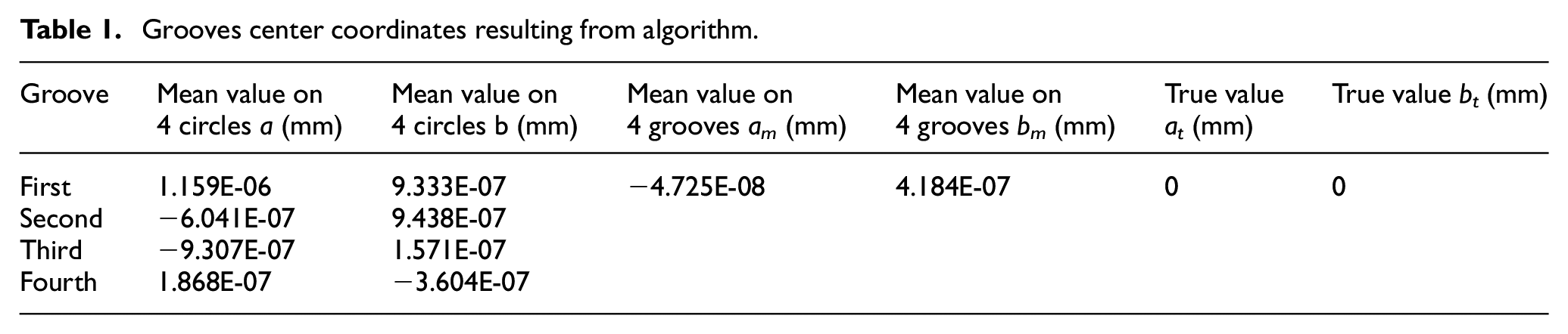
As synthetic tire was centered in the origin of the reference system, the first verification was performed on the ideal tire evaluating the mean value of the center coordinates referred to the four grooves (as shown in Figure 13) considering four circles for each of them. The calculated data, reported in Table 1, confirm the high reliability of the algorithm.

Figure 13.

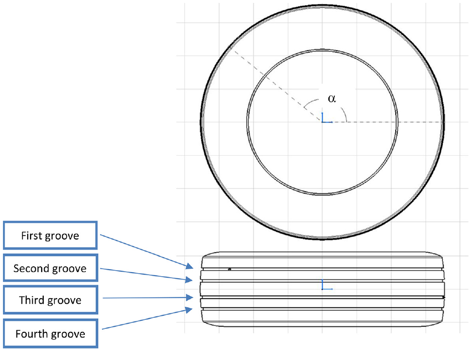
Schematic tire’s representation.

Table 1.

Grooves center coordinates resulting from algorithm.

Groove	Mean value on 4 circles a (mm)	Mean value on 4 circles b (mm)	Mean value on 4 grooves a_m (mm)	Mean value on 4 grooves b_m (mm)	True value a_t (mm)	True value b_t (mm)
First	1.159E-06	9.333E-07	−4.725E-08	4.184E-07	0	0
Second	−6.041E-07	9.438E-07
Third	−9.307E-07	1.571E-07
Fourth	1.868E-07	−3.604E-07

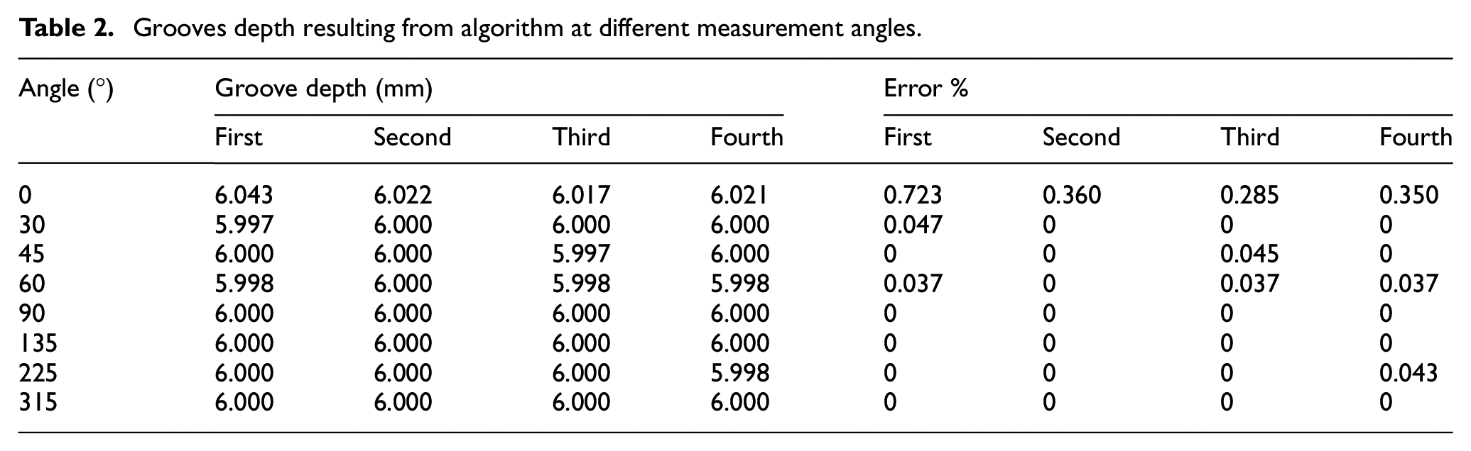
The second test was carried out on groove depth values at different α angles (see Figure 13). The resulting values of groove depth are resumed in Table 2 from which it is possible to observe that the error, respect to the true value of 6 mm, is always lower than 1%.

Table 2.

Grooves depth resulting from algorithm at different measurement angles.

Angle (°)	Groove depth (mm)				Error %
Angle (°)	First	Second	Third	Fourth	First	Second	Third	Fourth
0	6.043	6.022	6.017	6.021	0.723	0.360	0.285	0.350
30	5.997	6.000	6.000	6.000	0.047	0	0	0
45	6.000	6.000	5.997	6.000	0	0	0.045	0
60	5.998	6.000	5.998	5.998	0.037	0	0.037	0.037
90	6.000	6.000	6.000	6.000	0	0	0	0
135	6.000	6.000	6.000	6.000	0	0	0	0
225	6.000	6.000	6.000	5.998	0	0	0	0.043
315	6.000	6.000	6.000	6.000	0	0	0	0

Case 2: Defective and not worn tire

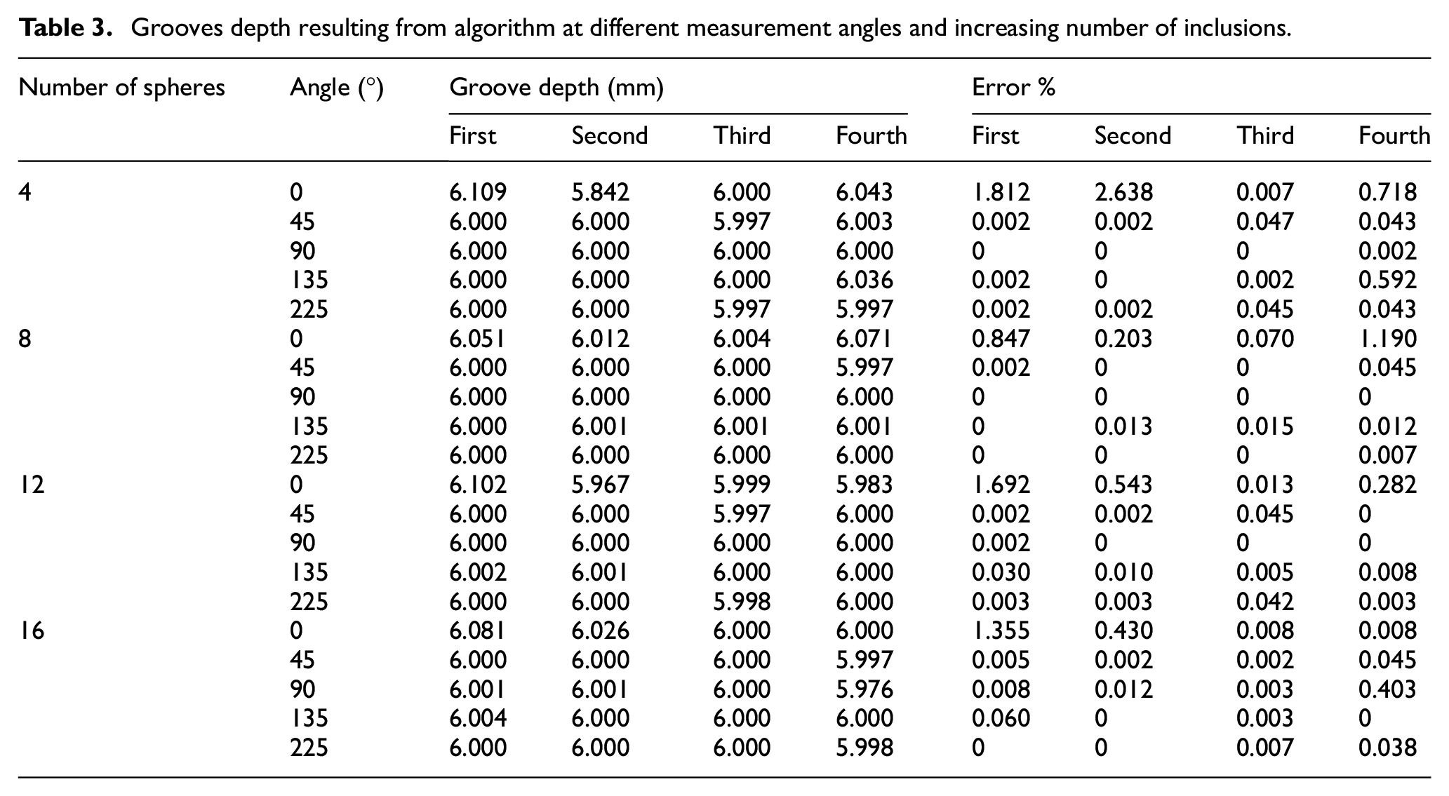
In the defective tire the inclusions are modeled as spheres of radius 3.5 mm, positioned on the second groove for α = 0° and on the fourth groove for α = 140° (Figure 14(a)). The analysis was performed for an increasing number of spheres from 4 to 16 adding two spheres at a time for groove and evaluating the groove depth measured at different α values. Concerning the center coordinates evaluation, the error resulted in the order of tenths of a millimeter in the worst case and, for brevity, the authors avoid reporting the relative tabular data. Table 3 reports the values of groove depth for all cases considered, showing an error lower than 3%.

Figure 14.

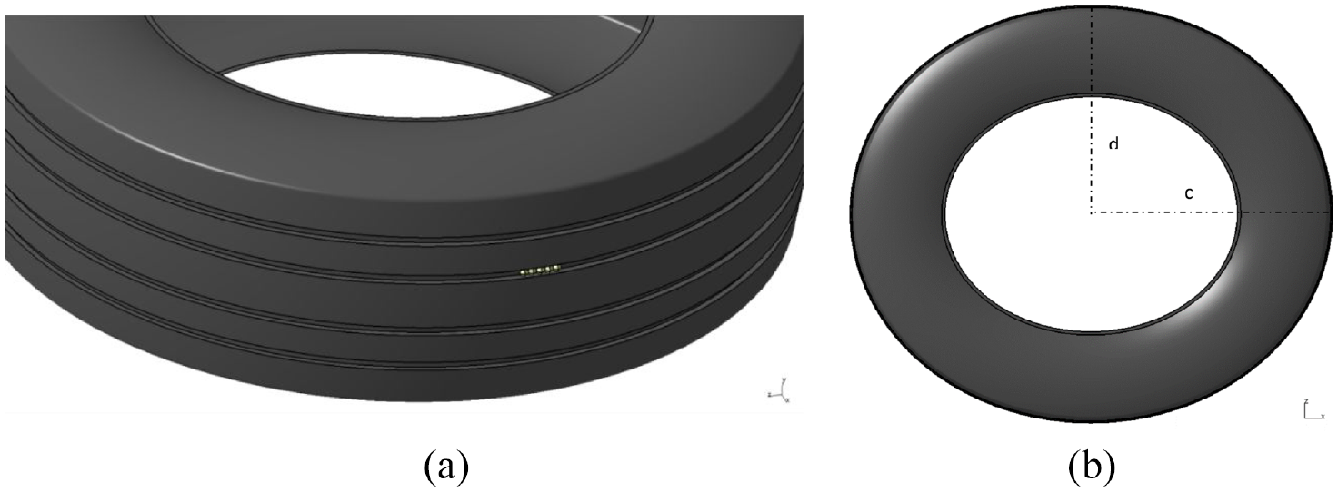
Synthetic tire with inclusions (a) and ovalization (b).

Table 3.

Grooves depth resulting from algorithm at different measurement angles and increasing number of inclusions.

Number of spheres	Angle (°)	Groove depth (mm)				Error %
Number of spheres	Angle (°)	First	Second	Third	Fourth	First	Second	Third	Fourth
4	0	6.109	5.842	6.000	6.043	1.812	2.638	0.007	0.718
	45	6.000	6.000	5.997	6.003	0.002	0.002	0.047	0.043
	90	6.000	6.000	6.000	6.000	0	0	0	0.002
	135	6.000	6.000	6.000	6.036	0.002	0	0.002	0.592
	225	6.000	6.000	5.997	5.997	0.002	0.002	0.045	0.043
8	0	6.051	6.012	6.004	6.071	0.847	0.203	0.070	1.190
	45	6.000	6.000	6.000	5.997	0.002	0	0	0.045
	90	6.000	6.000	6.000	6.000	0	0	0	0
	135	6.000	6.001	6.001	6.001	0	0.013	0.015	0.012
	225	6.000	6.000	6.000	6.000	0	0	0	0.007
12	0	6.102	5.967	5.999	5.983	1.692	0.543	0.013	0.282
	45	6.000	6.000	5.997	6.000	0.002	0.002	0.045	0
	90	6.000	6.000	6.000	6.000	0.002	0	0	0
	135	6.002	6.001	6.000	6.000	0.030	0.010	0.005	0.008
	225	6.000	6.000	5.998	6.000	0.003	0.003	0.042	0.003
16	0	6.081	6.026	6.000	6.000	1.355	0.430	0.008	0.008
	45	6.000	6.000	6.000	5.997	0.005	0.002	0.002	0.045
	90	6.001	6.001	6.000	5.976	0.008	0.012	0.003	0.403
	135	6.004	6.000	6.000	6.000	0.060	0	0.003	0
	225	6.000	6.000	6.000	5.998	0	0	0.007	0.038

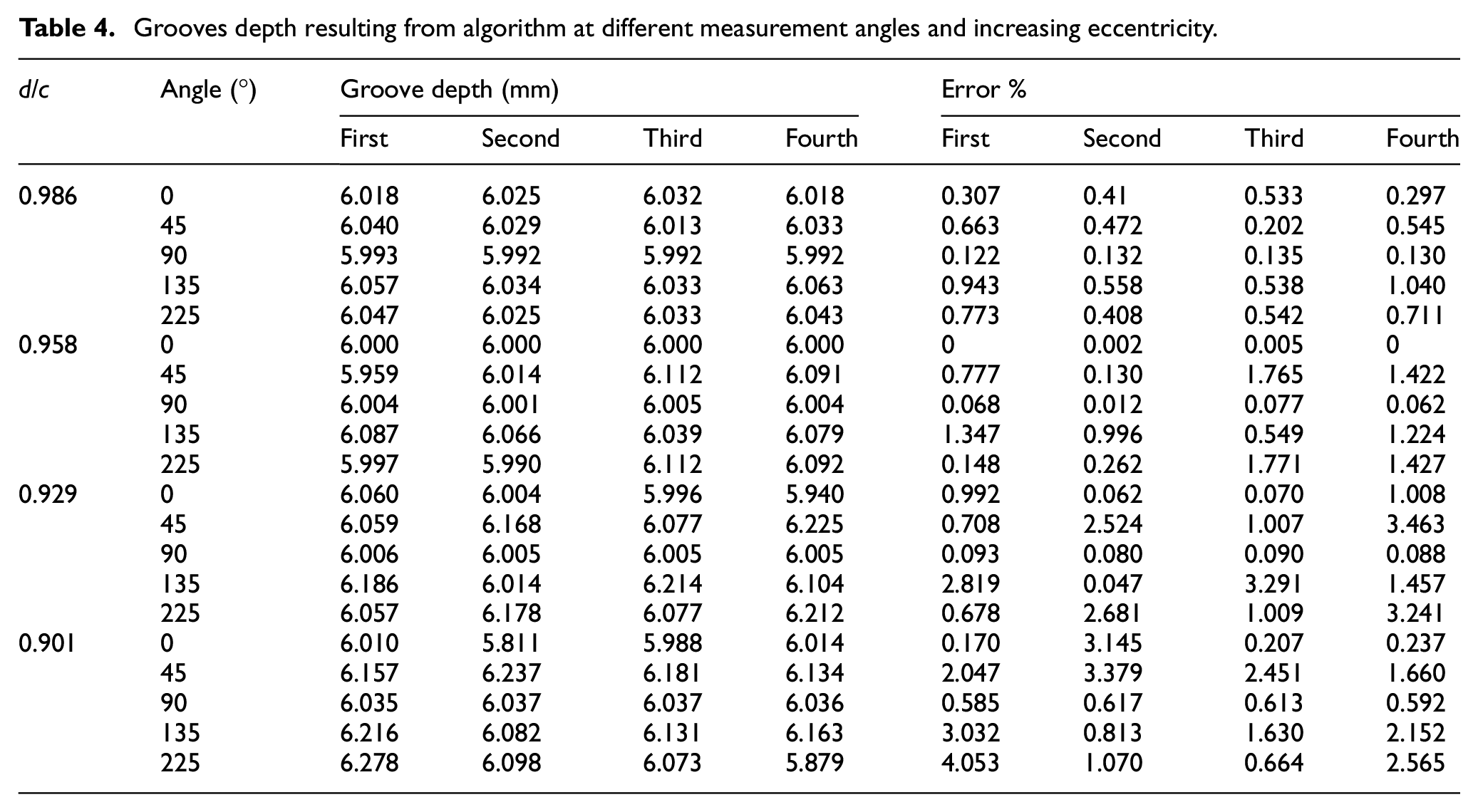
The last test is applied to an ovalized tire (Figure 14(b)). Several values of the eccentricity d/c, where c is the major semi axis and d the minor semi axis, were considered up to a minimum value equal to 0.9 and resulting for a difference between the semi axes equal to 35 mm. The evaluation was also performed for different α angles (Table 4) and the agreement with true values, measured on CATIA V5^® ovalized model, was excellent with a maximum error of 5% for the most severe ovalization.

Table 4.

Grooves depth resulting from algorithm at different measurement angles and increasing eccentricity.

d/c	Angle (°)	Groove depth (mm)				Error %
d/c	Angle (°)	First	Second	Third	Fourth	First	Second	Third	Fourth
0.986	0	6.018	6.025	6.032	6.018	0.307	0.41	0.533	0.297
	45	6.040	6.029	6.013	6.033	0.663	0.472	0.202	0.545
	90	5.993	5.992	5.992	5.992	0.122	0.132	0.135	0.130
	135	6.057	6.034	6.033	6.063	0.943	0.558	0.538	1.040
	225	6.047	6.025	6.033	6.043	0.773	0.408	0.542	0.711
0.958	0	6.000	6.000	6.000	6.000	0	0.002	0.005	0
	45	5.959	6.014	6.112	6.091	0.777	0.130	1.765	1.422
	90	6.004	6.001	6.005	6.004	0.068	0.012	0.077	0.062
	135	6.087	6.066	6.039	6.079	1.347	0.996	0.549	1.224
	225	5.997	5.990	6.112	6.092	0.148	0.262	1.771	1.427
0.929	0	6.060	6.004	5.996	5.940	0.992	0.062	0.070	1.008
	45	6.059	6.168	6.077	6.225	0.708	2.524	1.007	3.463
	90	6.006	6.005	6.005	6.005	0.093	0.080	0.090	0.088
	135	6.186	6.014	6.214	6.104	2.819	0.047	3.291	1.457
	225	6.057	6.178	6.077	6.212	0.678	2.681	1.009	3.241
0.901	0	6.010	5.811	5.988	6.014	0.170	3.145	0.207	0.237
	45	6.157	6.237	6.181	6.134	2.047	3.379	2.451	1.660
	90	6.035	6.037	6.037	6.036	0.585	0.617	0.613	0.592
	135	6.216	6.082	6.131	6.163	3.032	0.813	1.630	2.152
	225	6.278	6.098	6.073	5.879	4.053	1.070	0.664	2.565

Case 3: Ideal tire subjected to uniform wear phenomena

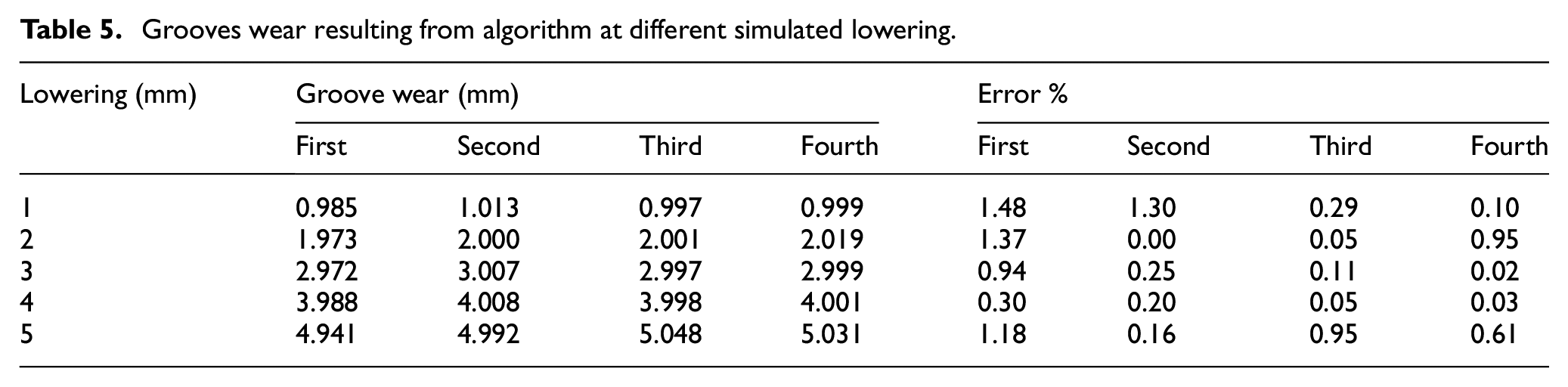
Starting from the ideal tire studied in Section 4.1, uniform wear tires have been obtained leaving unchanged the radial position of the groove and reducing the tire external radius of 1, 2, 3, 4, and 5 mm. These values of lowering correspond reasonably to the wear that averagely occurs after a driving cycle of 10,000 km on standard route. Figure 15 compares the different wear tire profiles with respect to the ideal tire. The wear and the relative error for each groove, reported in Table 5, are calculated respect to the groove depth value obtained from the algorithm on the ideal tire for α = 180°. The wear evaluation results very reliable considering that the maximum error is less than 1.5%.

Figure 15.

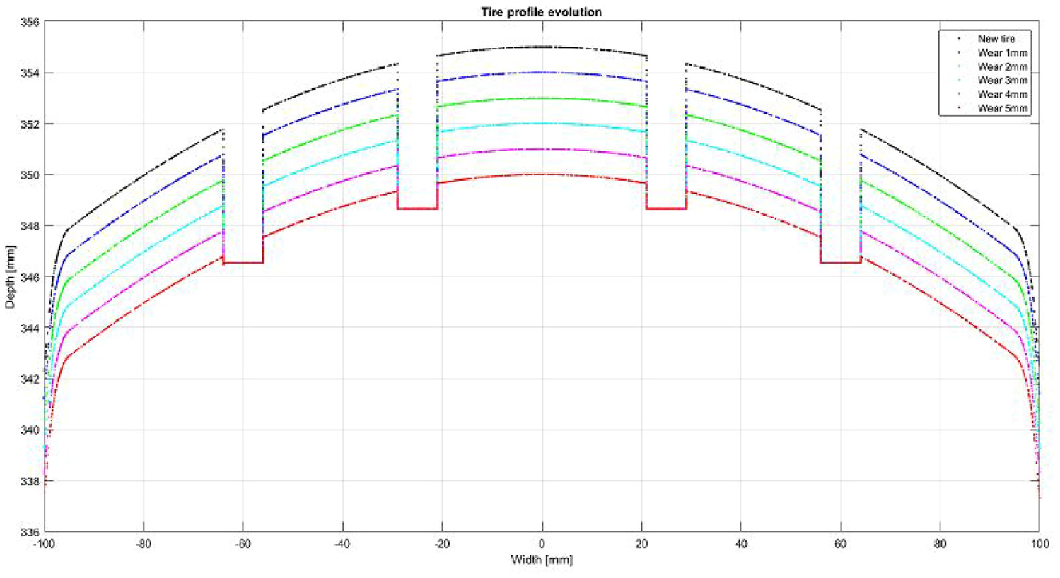
Tire profile evolution for increasing wear.

Table 5.

Grooves wear resulting from algorithm at different simulated lowering.

Lowering (mm)	Groove wear (mm)				Error %
Lowering (mm)	First	Second	Third	Fourth	First	Second	Third	Fourth
1	0.985	1.013	0.997	0.999	1.48	1.30	0.29	0.10
2	1.973	2.000	2.001	2.019	1.37	0.00	0.05	0.95
3	2.972	3.007	2.997	2.999	0.94	0.25	0.11	0.02
4	3.988	4.008	3.998	4.001	0.30	0.20	0.05	0.03
5	4.941	4.992	5.048	5.031	1.18	0.16	0.95	0.61

Experimental verification

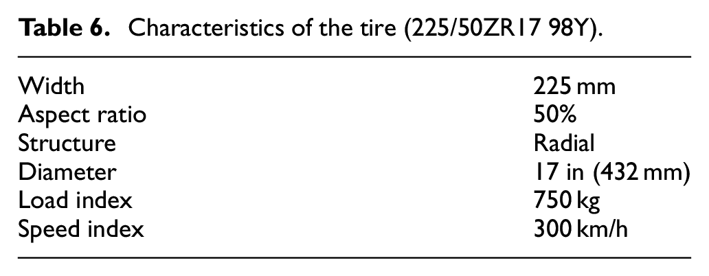
In this final section the methodology is applied for measuring the tread wear on a real tire. This is the right rear tire of a medium-sized sedan, whose characteristics are shown in Table 6.

Table 6.

Characteristics of the tire (225/50ZR17 98Y).

Width	225 mm
Aspect ratio	50%
Structure	Radial
Diameter	17 in (432 mm)
Load index	750 kg
Speed index	300 km/h

The first scan was carried out when the tire had already traveled about 12,000 km, while the second was done when the tire had covered a further 5395 km. The 3D acquisition of the tire geometry was carried out by using the structured light scanner DAVID SLS-2, which is characterized by a scan size of 60–500 mm, a resolution up to 0.05 mm, a scanning time for one single scan within 2 s (or up to 10 s, depending on settings and computer speed). Table 7 reports the set-up parameters of the scanning equipment.

Table 7.

Experimental set-up parameters.

Test set-up
Distance projector-camera	450 mm, with camera located on the right of the projector
Camera tilt angle	22° counterclockwise
Distance scanner-tire	650 mm
Calibration matrix size	240 mm

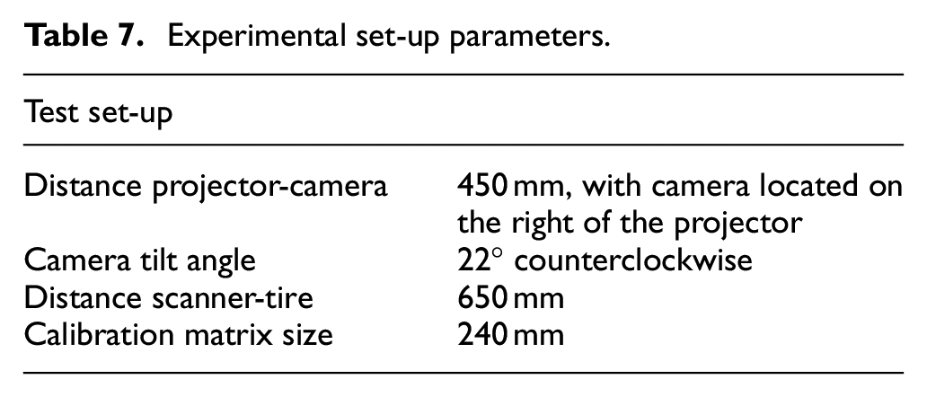
In general, the reconstruction of the 3D geometry of a scanned body is carried out in several steps. By using the set-up parameters of Table 7, 12 single scans were performed to obtain a complete description of the tire geometry. These different scans must be combined under the same coordinate system by a process called registration.

This process is performed usually two views at a time, according to the following two main steps:

- a first preliminary registration carried out by selecting three or more corresponding points on the two different clouds;

- a fine registration by means of the Iterative Closest Point (ICP) algorithm, which, iteratively, searches the configuration minimizing the sum of the squared distances of the points of the two clouds.

In the specific case of the tire, the regularity of the geometry, however, makes the preliminary registration a quite challenging process.

For this reason, a series of reference markers was added to the tread surface, which was scanned by using the option for the acquisition of the texture, that is available in the “Scan” environment of the software. Moreover, the tire was placed on a support specially designed (Figure 16) to fix the tire position from scan Before Test (BT) to scan After Test (AT).

Figure 16.

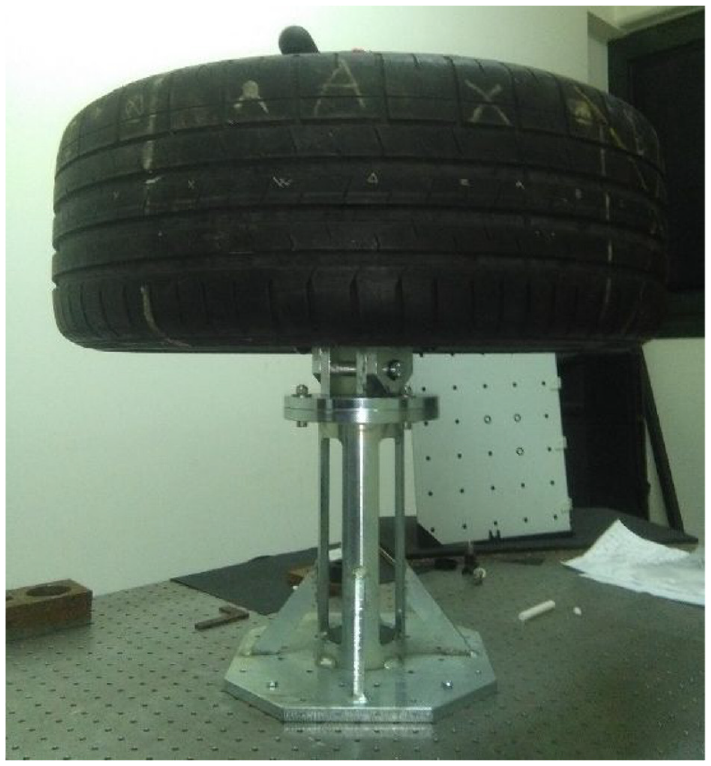
Marked tire on support.

The alignment of the individual scans was carried out taking advantage of the possibility, offered by the presence of the markers, to select a point common to the individual tire portions, obtaining the complete model.

After the registration, the various point clouds were merged to obtain a single mesh. Mesh editing operations, such as hole filling and smoothing, were also necessary to repair several types of detects. The final result of these experimental measurements was reported in Figure 17 (Before Test and After Test respectively). The 3D acquisition of the tire, including the preparation of the tire, the set-up of the scanning equipment the calibration phase, and the mesh defects editing, had a duration between 20 and 25 min, allowing to obtain a final triangular mesh of about 1.5 × 10⁶ vertices.

Figure 17.

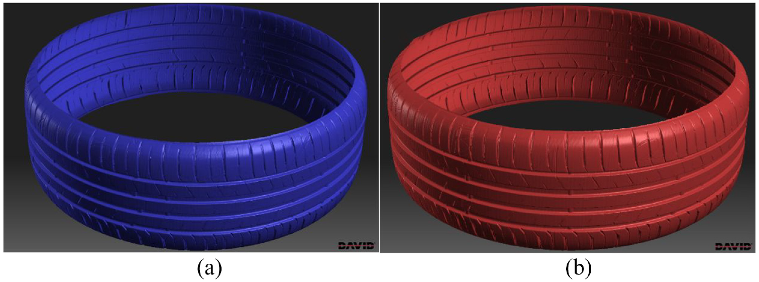
Result at the end of the merging process in the tire Before Test (a) and After Test (b).

To quantify the wear status of the tire, four tread profiles angularly equidistant on the tire circumference were extracted by using the data processing algorithm before described. These profiles allow to obtain the groove depths at four angular positions and to compare them before and after the driving cycle. From this comparison, it was possible to obtain an estimation of the tread wear, with a measurement method similar to that used for the calculation of the tread wear index in the UTQG (Uniform Tire Quality Grading) system.³¹

In order to identify the angular position of the profile, the axis x of this reference (Figure 18(a)) is placed at one specific vertex of the tread wear indicator triangle (TWI in Figure 18(b)), which is located in an area not in contact with the road surface.

Figure 18.

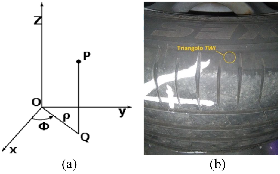
Identification of the cylindrical coordinate system (a) using the tread wear indicator on the tire surface (b).

By this methodology four equally spaced profiles have been extracted for axial plane angularly located at 0°, 90°, 180°, and 270°. In particular, an angular sector of width β equal to 0.2° was chosen to obtain a robust measurement and, at the same time, to ensure a high point density of the extracted profile. Figures 19 and 20 show, as example, the profile and individual grooves subplots for α = 0° respectively for BT tire (in blue), and AT tire (in red).

Figure 19.

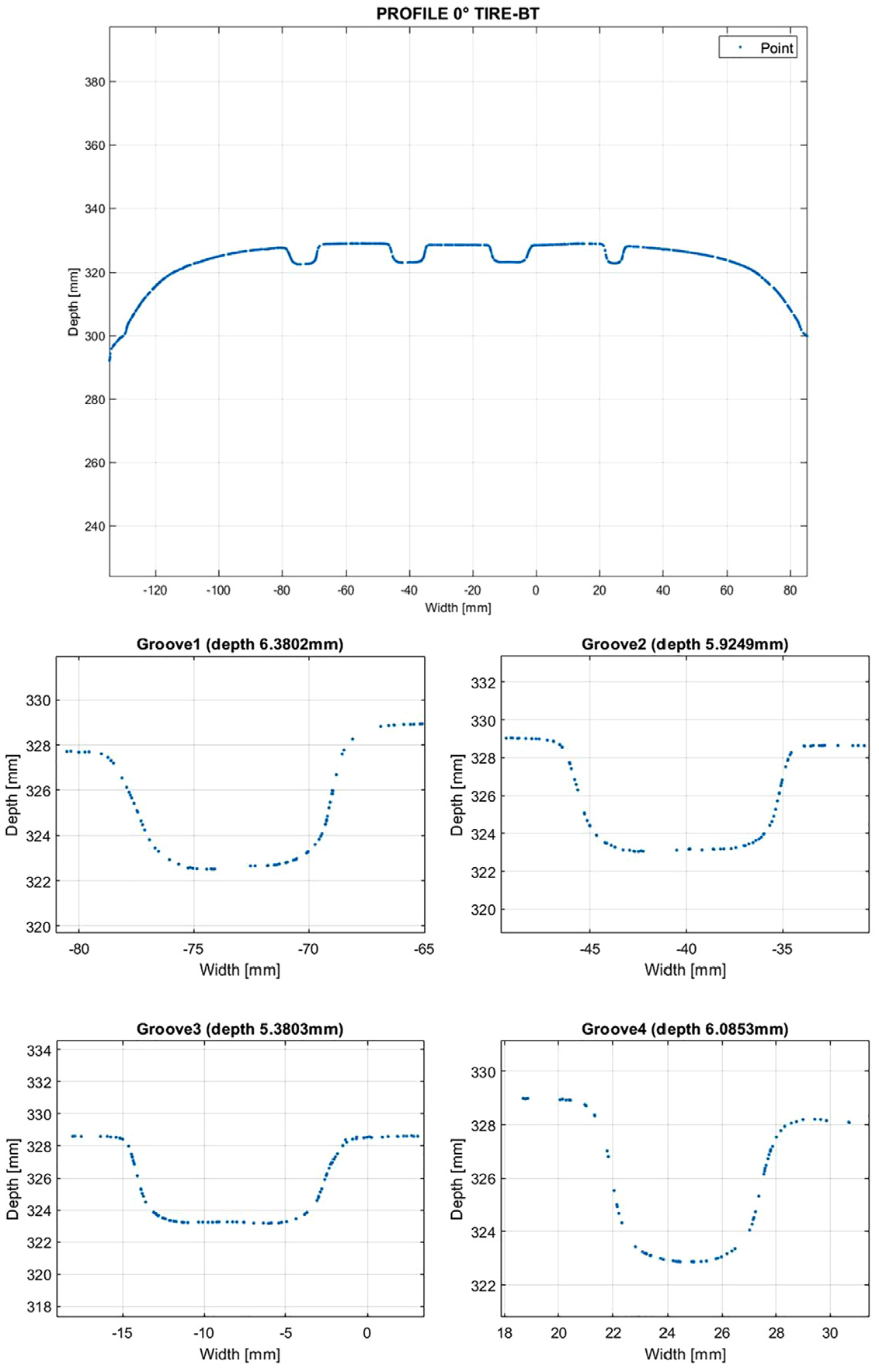
Profile and individual grooves subplots in the tire before test (BT) for α = 0°.

Figure 20.

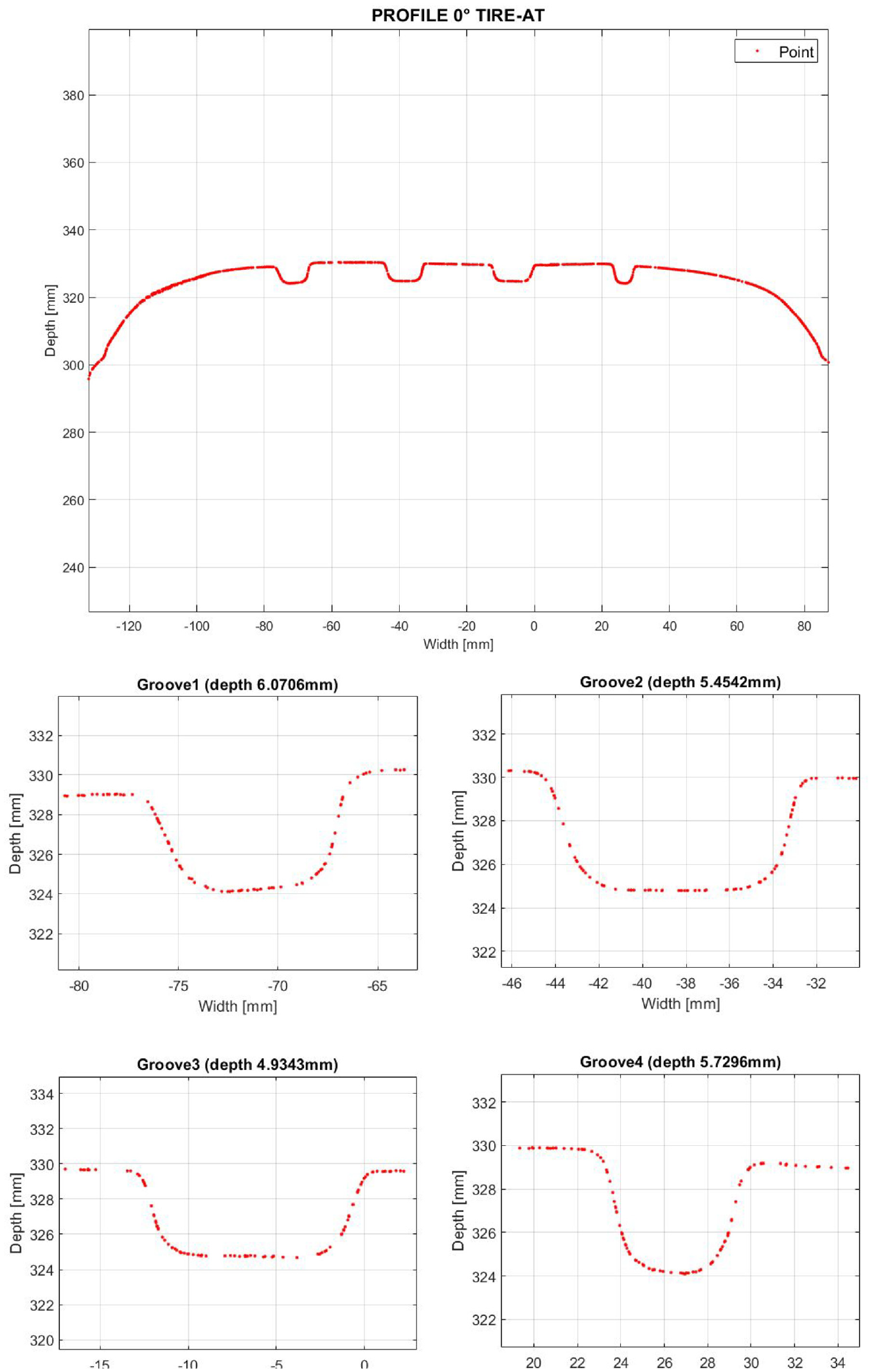
Profile and individual grooves subplots in the tire after test (AT) for α = 0°.

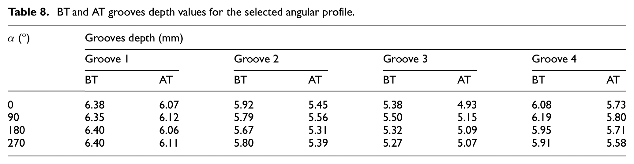
Finally, Table 8 shows the results of the measurements on four grooves for each anomaly and Table 9 reports the values obtained for the tread lowering or each groove and anomaly. From these data the lowering of the tire thickness, that is, the tire wear, results approximately equal to 0.3–0.4 mm for a driving test of about 5000 km. This wear value is realistic if it is considered that a mileage of 50,000 km causes the complete wear of a tire, that is, a tread lowering of 3 mm. Evaluating the tread lowering for different anomaly values allows to establish if the wear of the tire is uniform or not and then to determine the type of wear state referring to Figure 1. For the test performed here, for example, the wear can be considered quite uniform.

Table 8.

BT and AT grooves depth values for the selected angular profile.

α (°)	Grooves depth (mm)
	Groove 1		Groove 2		Groove 3		Groove 4
	BT	AT	BT	AT	BT	AT	BT	AT
0	6.38	6.07	5.92	5.45	5.38	4.93	6.08	5.73
90	6.35	6.12	5.79	5.56	5.50	5.15	6.19	5.80
180	6.40	6.06	5.67	5.31	5.32	5.09	5.95	5.71
270	6.40	6.11	5.80	5.39	5.27	5.07	5.91	5.58

Table 9.

Tread lowering for each groove and anomaly.

α (°)	Tread lowering (mm)
α (°)	Groove 1	Groove 2	Groove 3	Groove 4
0	0.31	0.47	0.45	0.35
90	0.23	0.23	0.35	0.39
180	0.34	0.36	0.23	0.24
270	0.29	0.41	0.20	0.33
Mean value	0.29	0.37	0.31	0.33
St. dev.	0.046458	0.102103	0.115	0.063443

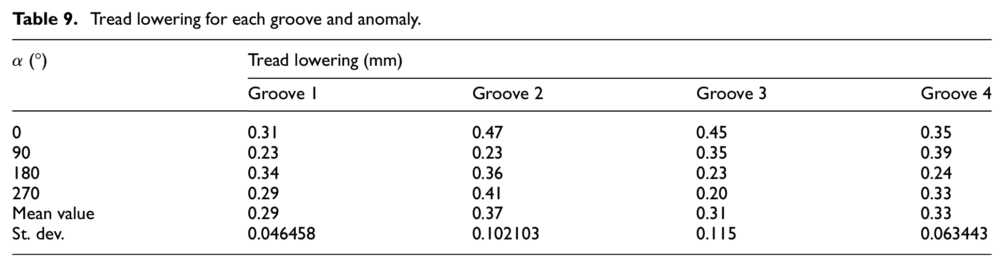
A statistical analysis was carried out on experimental data using a one-way ANOVA test. The considered groups are the wear measurements at different angles obtaining the results in Table 10.

Table 10.

ANOVA test results.

	Sum of squares	Degrees of freedom	Mean square	F-value	a ₀	p Value
Between groups	0.027525	3	0.009175	1.47	0.05	0.27
Within groups	0.074650	12	0.006221

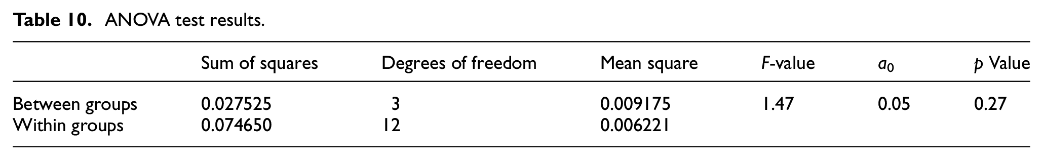
The p-value results higher than interval confidence α₀, and so we accept the null hypothesis, and conclude that there are not significant differences between the groups.

Conclusions

This work was aimed at developing a reliable, semi-automatic, and low-cost tool for tire wear measurement suitable for industrial applications:

- a measurement set up based on a 3D structured light scanner for the 3D acquisition of the tread geometry was developed;

- a semi-automatic algorithm for processing the points cloud experimentally acquired was implemented in MATLAB^®;

- several case studies were modeled into CATIA V5^® to test the methodology under several conditions. The algorithm has proved to be robust even in the case of a defective tire;

- finally, a first application of the algorithm for wear evaluation was performed on a real tire obtaining satisfying results in terms of reliability.

Footnotes

Acknowledgements

The authors warmly acknowledge Antonio Toma, Pierpaolo Positano, and Antonio Gratis of Nardò Technical Center s.r.l. for their technical support and suggestions.

Declaration of conflicting interests

The author(s) declared no potential conflicts of interest with respect to the research, authorship, and/or publication of this article.

Funding

The author(s) received no financial support for the research, authorship, and/or publication of this article.

ORCID iD

Marta De Giorgi

References

Deng

Zhan

Liu

, et al. Multiscale power spectrum analysis of 3D surface texture for prediction of asphalt pavement friction. Constr Build Mater 2021; 293: 123506.

Liu

Zhan

Deng

, et al. An improved differential box counting method to measure fractal dimensions for pavement surface skid resistance evaluation. Measurement 2021; 178: 109376.

Akkök

Acar

Açmaz

Experimental analysis and wear modeling for mechanical components of a typical rail launcher. Wear 2013; 306: 1–9.

Stachowiak

Batchelor

Stachowiak

GB.

Experimental methods in tribology. Tribol Ser 2004; 44: 27–29.

Bills

Blunt

Jiang

Development of a technique for accurately determining clinical wear in explanted total hip replacements. Wear 2007; 263: 1133–1137.

Brunskill

Harper

Lewis

The real-time measurement of wear using ultrasonic reflectometry. Wear 2015; 332: 1129–1133.

Birring

Kwun

Ultrasonic measurement of wear. Tribol Int 1989; 22: 33–37.

Castejón

Alegre

Barreiro

, et al. Online tool wear monitoring using geometric descriptors from digital images. Int J Mach Tools Manuf 2007; 47: 1847–1853.

Dutta

Pal

Mukhopadhyay

, et al. Application of digital image processing in tool condition monitoring: a review. CIRP J Manuf Sci Technol 2013; 6: 212–232.

10.

Hamed

El Ghandoor

El Diasty

, et al. Analysis of speckle images to assess surface roughness. Opt Laser Technol 2004; 36: 249–253.

11.

Valigi

Logozzo

Rinchi

Wear resistance of blades in planetary concrete mixers. Design of a new improved blade shape and 2D validation. Tribol Int 2016; 96: 191–201.

12.

Valigi

Fabi

Gasperini

. Wear resistance of new blade for planetary concrete mixer. In: Proceedings of the 5th world tribology congress, Torino, Italy, 8–13 September 2013.

13.

Pawley

JB.

Handbook of biological confocal microscopy. New York, NY: Springer, 2006, pp.1–19.

14.

El-Hakim

Beraldin

Blais

. A Comparative evaluation of the performance of passive and active 3-D vision systems. In: SPIE, 2646-conference on digital photogrammetry and remote, St. Petersburg, VA, USA, 25–30 June 1995.

15.

Valigi

Logozzo

Affatato

New challenges in tribology: wear assessment using 3D optical scanners. Materials 2017; 10: 548.

16.

Dong

Sun

, et al. A feature-based method for tire pattern reverse modeling. Adv Eng Softw 2018; 124: 73–89.

17.

Wang

, et al. The study on tire tread depth measurement method based on machine vision. Adv Mech Eng 2019; 11: 1–12.

18.

Uffenkamp

Wingbermuehle

Nobis

, et al. Device and method for measuring the tread depth of a tire. Patent US20150330773, 2015.

19.

Carmignato

Spinelli

Affatato

, et al. Uncertainty evaluation of volumetric wear assessment from coordinate measurements of ceramic hip joint prostheses. Wear 2011; 270: 584–590.

20.

Bassani

Ciulli

Manfredi

, et al. Experimental study on wear and fracture in aeronautical gear transmissions. In: 8th Biennial ASME conference on engineering systems design and analysis, Torino, Italy, 4–7 July 2006.

21.

Uddin

MS.

Wear measurement and assessment of explanted cross-linked PE acetabular cups using a CMM. Tribol Trans 2014; 57: 767–777.

22.

Uddin

Mak

Callary

SA.

Evaluating hip implant wear measurements by CMM technique. Wear 2016; 364–365: 193–200.

23.

Bhushan

. Micro/nanotribology: state of the art and its applications. In: NSF/AFOSR/ASME workshop on tribology issues and opportunities in MEMS, Columbus, OH, USA, 9–11 November 1997.

24.

Bassani

Ciulli

Labardi

, et al. Wear analysis of journal bearing coatings by atomic force microscopy. Metall Ital 2002; 94: 37–44.

25.

Anderson

Hoffman

HH.

Laser gauge tire dimensional measurement system. In: Automotive engineering congress, 1974.

26.

Bell

Beiwen

Zhang

Structured light techniques and applications. In: Wiley-Interscience (ed.) Wiley encyclopedia of electrical and electronics engineering. Hoboken, NJ: John Wiley & Sons, 2016, pp.1–24.

27.

Schmalz

Robust single-shot structured light 3D scanning. PhD Thesis, Universitätsbibliothek der Universität Erlangen-Nürnberg, 2012.

28.

Fusiello

Visione computazionale: Tecniche di ricostruzione tridimensionale. Milano: Franco Angeli, 2018.

29.

Chernov

Circular and linear regression: fitting circles and lines by least squares. Boca Raton, FL: Taylor & Francis, 2010.

30.

Taubin

Estimation of planar curves, surfaces and nonplanar space curves defined by implicit equations, with applications to edge and range image segmentation. IEEE Trans Pattern Anal Mach Intell 1991; 13: 1115–1138.

31.

49 CFR § 575.104 - uniform tire quality grading standards.

A semi-automatic methodology for tire’s wear evaluation

Abstract

Keywords

Introduction

Tire geometry and wear evaluation

The methodology for tread wear evaluation

Preliminary tests

Case 1: Ideal and not worn tire

Case 2: Defective and not worn tire

Case 3: Ideal tire subjected to uniform wear phenomena

Experimental verification

Conclusions

Footnotes

Acknowledgements

Declaration of conflicting interests

Funding

ORCID iD

References