
Abstract
In the downhole oil and gas industry, temperature prediction is an important means to avoid the hazards brought by the high-temperature environment to electronic devices. An improved adaptive Kalman filter (IAKF) temperature prediction method, used here as a virtual sensor, can predict the instrument temperature in real time. It uses the temperature state transfer matrix as a system adaptive discriminant parameter to improve the prediction accuracy of the model. This approach is a data-driven prediction method for practical, field-deployable application, it does not require modeling of heat transfer mechanisms and does not require data sets. Experiments results show that the IAKF model can effectively predict the changing trend of the apparatus in the next 30 min, and the maximum temperature prediction error is within 6.5°C. Its predictions are more stable and accurate than the extended Kalman filter, and it consumes very little CPU resources to run in embedded devices.
Introduction
In the downhole oil and gas industry, high-temperature logging apparatus works at 200°C and above. Although passive thermal management has the advantage of being simple in structure and more reliable than active thermal management, passive thermal management can only slow down the internal heating process of logging instruments, moreover, traditional passive thermal management techniques take action only after the temperature reaches a threshold, so the instrument still faces high temperature damage in long-term operation. Thermal management of high-temperature logging apparatus is essential to ensure that the electronics inside the apparatus operate in the recommended temperature range, and is critical to efficient oil and gas exploration. 1 Passive thermal management has the advantages of simplicity and reliability compared to active thermal management. 2 Peng et al. 3 used phase change materials filled in the internal skeleton of a logging apparatus for cooling the heat source circuits, however passive management can only slow down the internal heating process and still faced high-temperature damage as its internal temperature continued to increase over time. Thermal prediction, as a major part of thermal management, is an important mean to avoid the high-temperature environment to bring harm to the electronic devices.4–7
In recent years, thermal prediction methods for electronic systems have been divided into two main approaches based on mathematical descriptions: physical modeling methods and black-box prediction methods. 8 Usually, physical modeling approaches ignore the high complexity of the model and require the determination of many physical parameters, 9 which is a difficult task to determine. And the black box prediction method has a better development. Athavale et al. 6 investigated three different data-driven model temperature prediction methods, namely artificial neural network (ANN), support vector machine (SVM), and Gaussian process regression (GPR), to predict the rack inlet air temperature distribution in data centers, and used a suitable orthogonal decomposition method (POD) for transient temperature modeling prediction of data center inlet air temperature distribution, where the GPR prediction model predicted the average temperature in data centers with an error of no more than 1°C.
Although machine learning-related thermal prediction methods have high prediction accuracy, they are deficient in the on-site application of thermal prediction for high-temperature logging apparatus. The high prediction accuracy of these machine learning algorithms relies on the computation of a large training set of data, and this computational complexity imposes a significant resource consumption on the downhole embedded devices. The goal of our technique is to prevent thermal problems at very low-performance overhead. To meet the demand for highly accurate, real-time temperature prediction for downhole embedded devices, we consider a data-driven Kalman filtering algorithm, in which the predicted value of temperature depends only on the temperature information of the previous moment. Compared with other thermal prediction models, Kalman filtering has the significant advantage of consuming less computational resources, fast computation, no data set required, 10 and can run in the embedded devices.11–17 And there are many improved Kalman filtering methods in recent years, such as hybrid simplified Kalman filter (H-SKF). 17 The extended Kalman filter method can effectively provide maximum likelihood estimation for nonlinear systems, 18 however, the extended Kalman filter suffers from low estimation accuracy and poor stability when solving nonlinear system prediction problems. To address this problem, an improved adaptive Kalman filter temperature prediction algorithm (IAKF) is designed and implemented, which uses the temperature state transfer matrix as the system adaptive discrimination parameter to accommodate the effect of the thermodynamic circulation process inside the instrument on the system state transfer matrix.
In this paper, we investigate how to use predictors to predict temperature, and the improved adaptive Kalman filter temperature prediction model is applied to the temperature prediction problem of high temperature logging instruments. To accommodate the influence of the complex thermodynamic circulation process inside the apparatus on the temperature prediction accuracy, the model uses the temperature state transfer matrix as the system adaptive discrimination parameter, which makes the model have high-temperature prediction accuracy. This approach is a data-driven prediction method for practical, field-deployable application, does not require modeling of the heat transfer mechanism, and does not require a data set. The second part of the article introduces the theoretical formulation of the extended Kalman filter for temperature prediction, the third part of the article presents the improved adaptive Kalman filter solution, pointing out the advantages and main features of the solution, the fourth part presents the experimental procedure and results, and the fifth part concludes the article.
Adaptive extended Kalman filter (AEKF) temperature prediction principle
The Kalman filter method is commonly used in prediction problems, and its application relies on the establishment of a state space model. The state space model consists of a state equation and an observation equation. Among them, the state equation describes the change and transfer of state (predictor) based on time series data; the observation equation updates the dynamic process of state transfer (correction) based on the observed values obtained from measurements.
In the instrument thermal temperature prediction problem, the temperature of the instrument at the next moment is unknown, however, it can be estimated by means of Kalman filtering, which can be considered as a state observer, a set of mathematical equations that provide an efficient recursive average to estimate the unknown state of a process (state vector). In general, to correctly estimate the process state, the state observer requires two steps: (1) a time update step (prediction) to obtain an initial estimate of the state vector from the knowledge of the process dynamics model and (2) a measurement update step (correction) that integrates sensor measurements to refine the initial estimate of the state vector. In other words, the state observer estimates a process by using a form of feedback control: the filter estimates the process state at some time and then obtains feedback in the form of a noisy measurement. For instrumental thermal temperature prediction, the Kalman filter method forms a virtual sensor that takes as input a time series of temperature change values to obtain predictive information about the temperature for a future period.
Inside the thermos, the temperature of the instrument only rises, so we can describe the nonlinear temperature state space model inside the logging instrument as 19
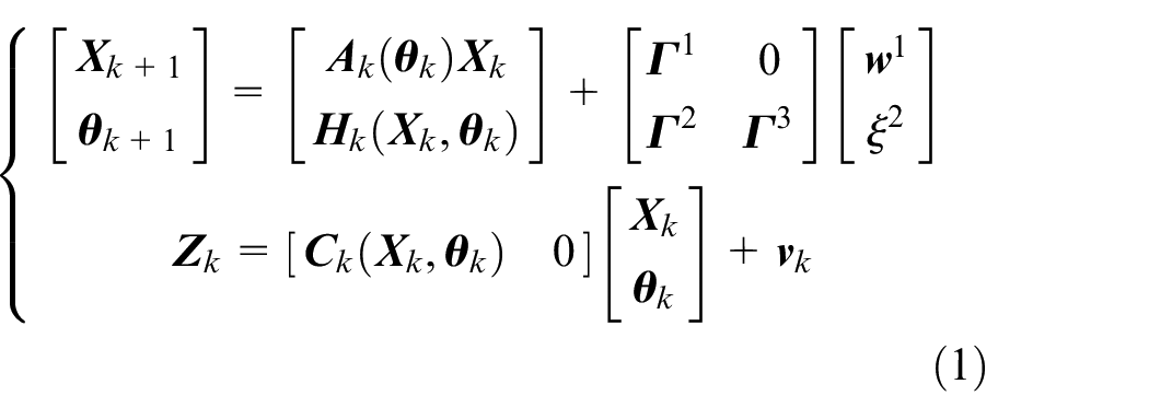
in the formula,
Algorithm I:
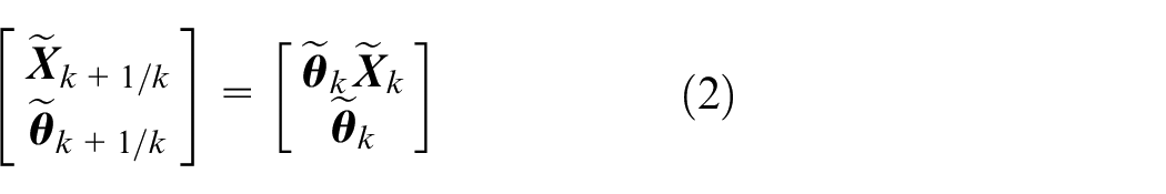
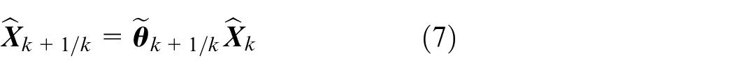
(1) One-step state prediction using the state transfer matrix
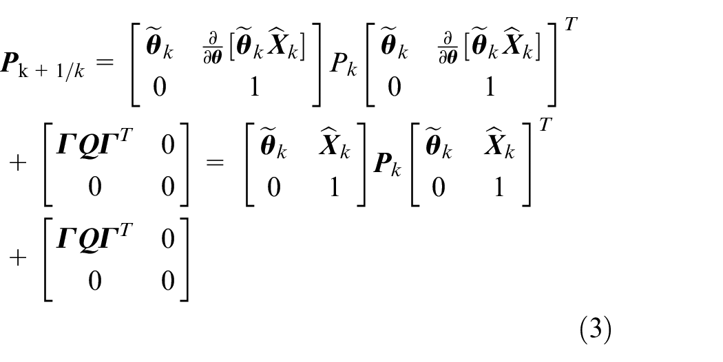
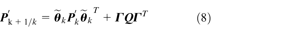
(2) State-step prediction covariance update:
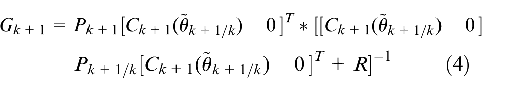
(3) Calculating the Kalman filter gain:
(4) State covariance update:
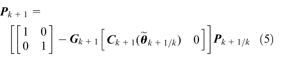
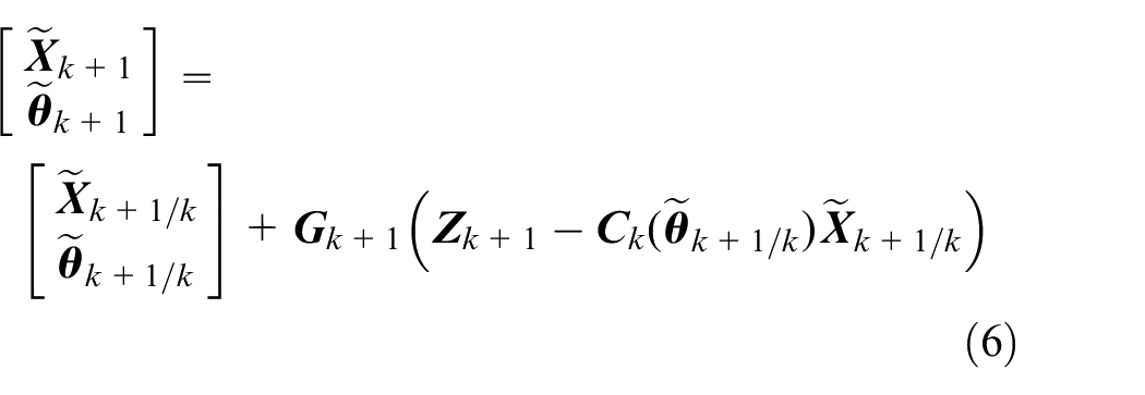
(5) State estimation parameter update:
Where the initial value of the state covariance
Algorithm II:
(1) State one-step prediction using the state transfer matrix
(2) State-step prediction covariance update:
(3) Calculating the Kalman filter gain:
(4) State covariance update:
(5) State estimation parameter update:
Where the initial value of the state covariance
AEKF individual circuit design.
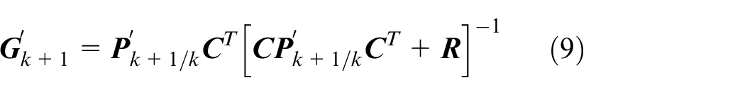
A flowchart of the AEKF algorithm is shown in Figure 2.
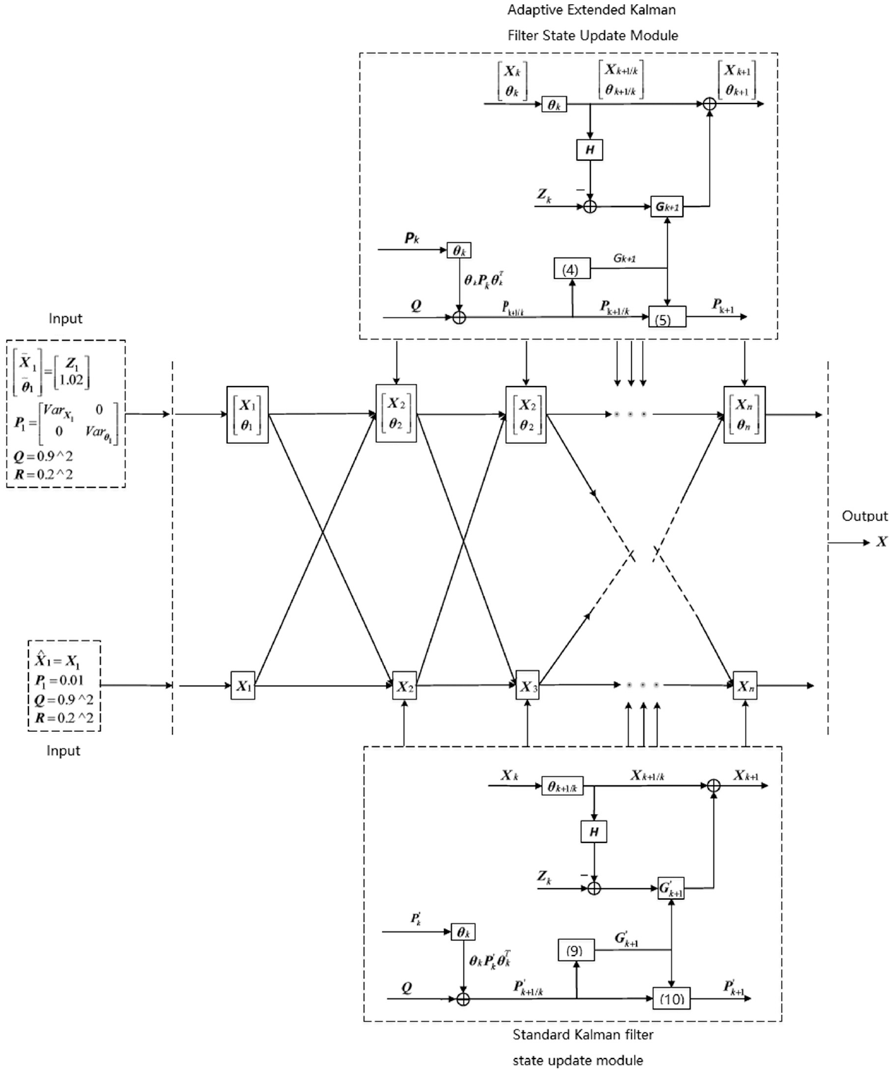
AEKF algorithm flow chart.
Intuitively, the IAKF algorithm is able to adjust the system state transfer matrix
Improved adaptive Kalman filter temperature prediction algorithm
Simplification of AEKF algorithm and proof of effectiveness
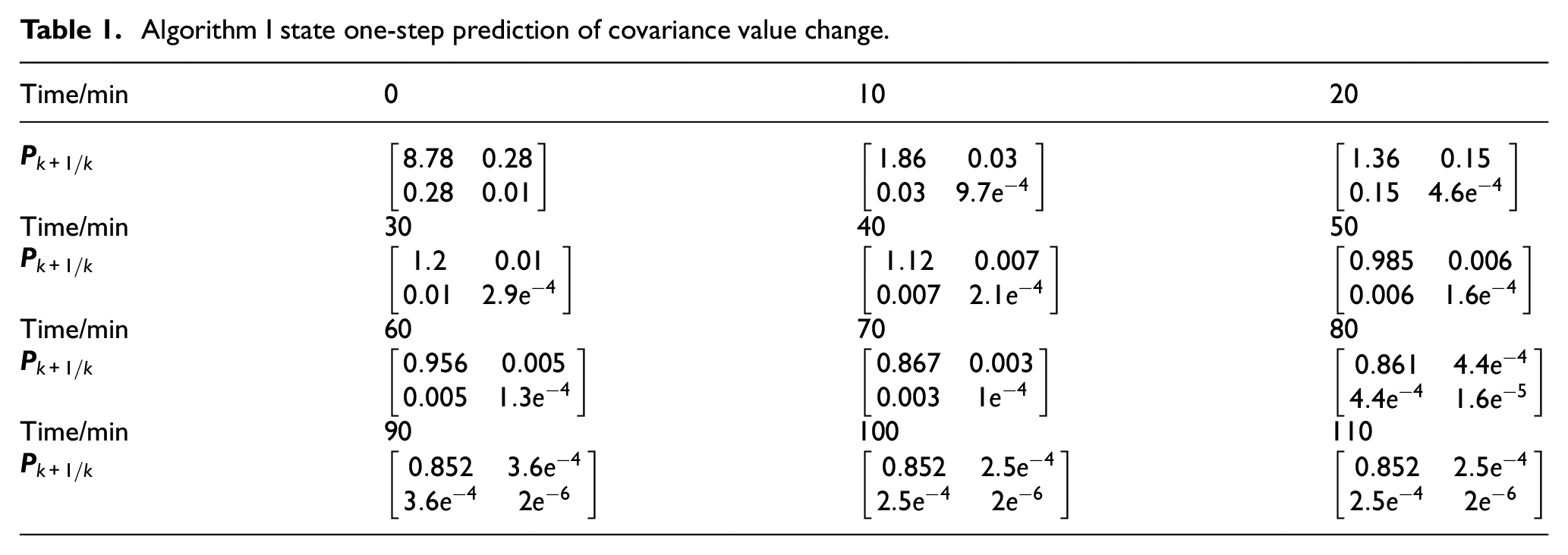
From Tables 1 and 2, it can be seen that:
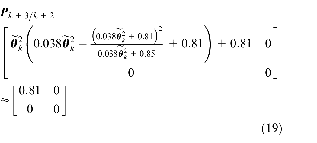
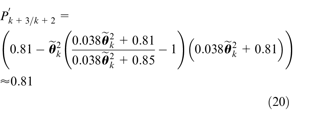
Theorem 3.1: The state one-step prediction covariance of the two sub-algorithms in AEKF tends to a constant term as the recurrence term increases, as
Algorithm I state one-step prediction of covariance value change.
Algorithm II State one-step prediction of covariance array value change.
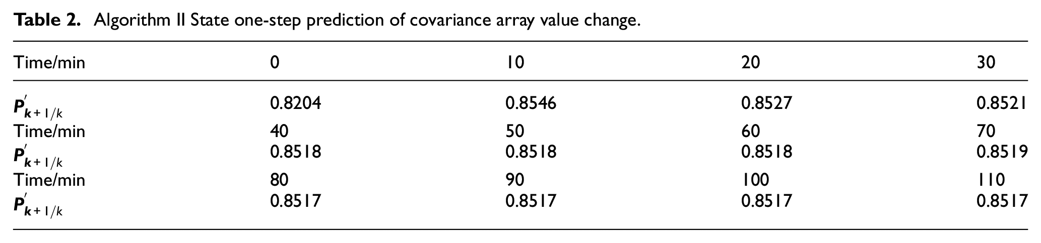
It is mainly due to the fact that the state one-step estimation error is very small during its calculation of the state one-step prediction covariance, and the state one-step prediction covariance mainly comes from the process noise term.
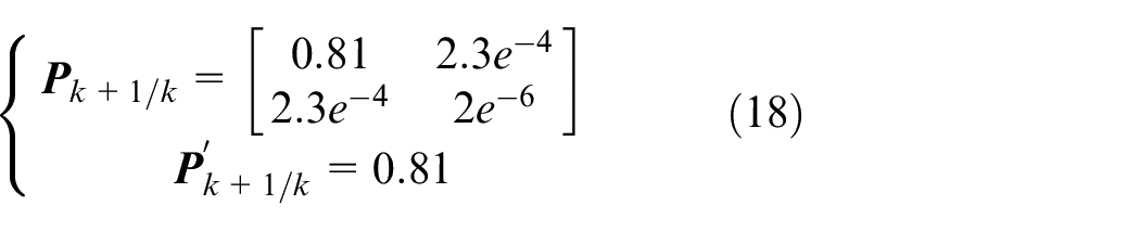
According to mathematical induction: (1) in the first step, it is clear from Tables 1 and 2 that the state one-step prediction covariance array of the two sub-algorithms in the AEKF algorithm is bounded and converges to a constant when k is recursive to the 10th term, that is,
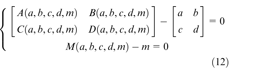
then the expressions of each element in
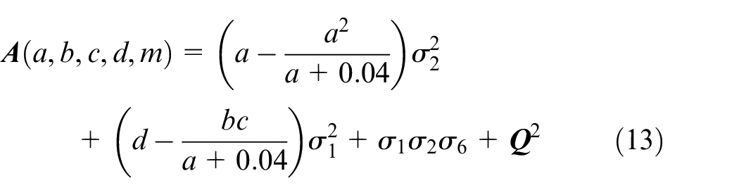
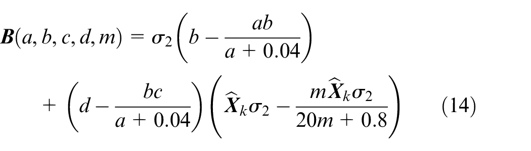
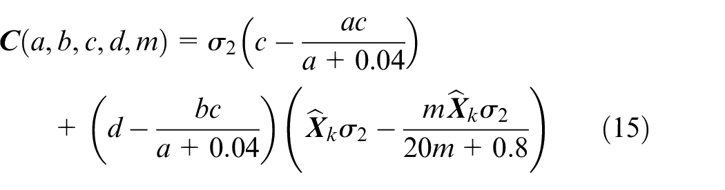
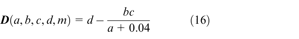
in the formula,
So
Proof of IAKF algorithm stability
To demonstrate that the simplified IAKF temperature prediction model can make effective estimates of the system state, the following stability proof is performed.
Theorem 3.2: The IAKF model is stable when the IAKF state one-step prediction covariance array is a constant and an upper bound exists for its state estimation mean squared error array
Proof:
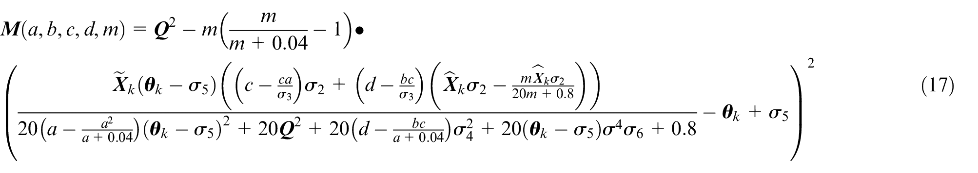
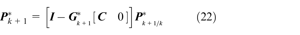
Based on Theorem 3.2, to describe the above IAKF algorithm the actual estimated mean squared error

According to Theorem 3.1 it is known that the simplified model is valid, and when the model is valid, according to the five basic equations in the adaptive extended Kalman filter. it is known that the true state estimation mean squared error array is
in the formula
Due to the simplification of the state estimation covariance array, a certain bias
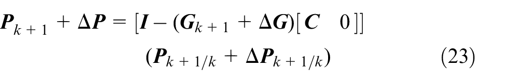
where

Bringing equation (24) into equation (23), we get
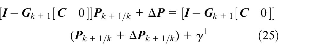
Among them
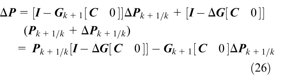
Since
Experimental and results
A high-temperature experiment was conducted to verify the adaptability of the proposed adaptive Kalman filter model. Commercial off-the-shelf components are widely used when developing instruments for high-temperature environments, but the behavior and high-temperature tolerance of each component needs to be carefully evaluated before use. Each chip in this design has been tested. The temperature acquisition and prediction circuit uses a TI DSP chip as the control and calculation core, model TMS320F2812, and the DSP chip operates at a main clock frequency of 30 MHz in order to ensure the stability of the circuit and DSP chip when running at high temperatures. The physical circuit board is shown in Figure 3(b), and to better avoid hot spot problems, the DSP chip and SRAM chip are packaged in system-in-package (SIP). Once the temperature information has been collected, the DSP chip completes the data processing based on the IAKF algorithm. The predicted temperature values calculated by DSP can be transmitted to the ground equipment through 1553B bus and drawn into a curve trend. The system block diagram of the ground information processing system are shown in Figure 4.
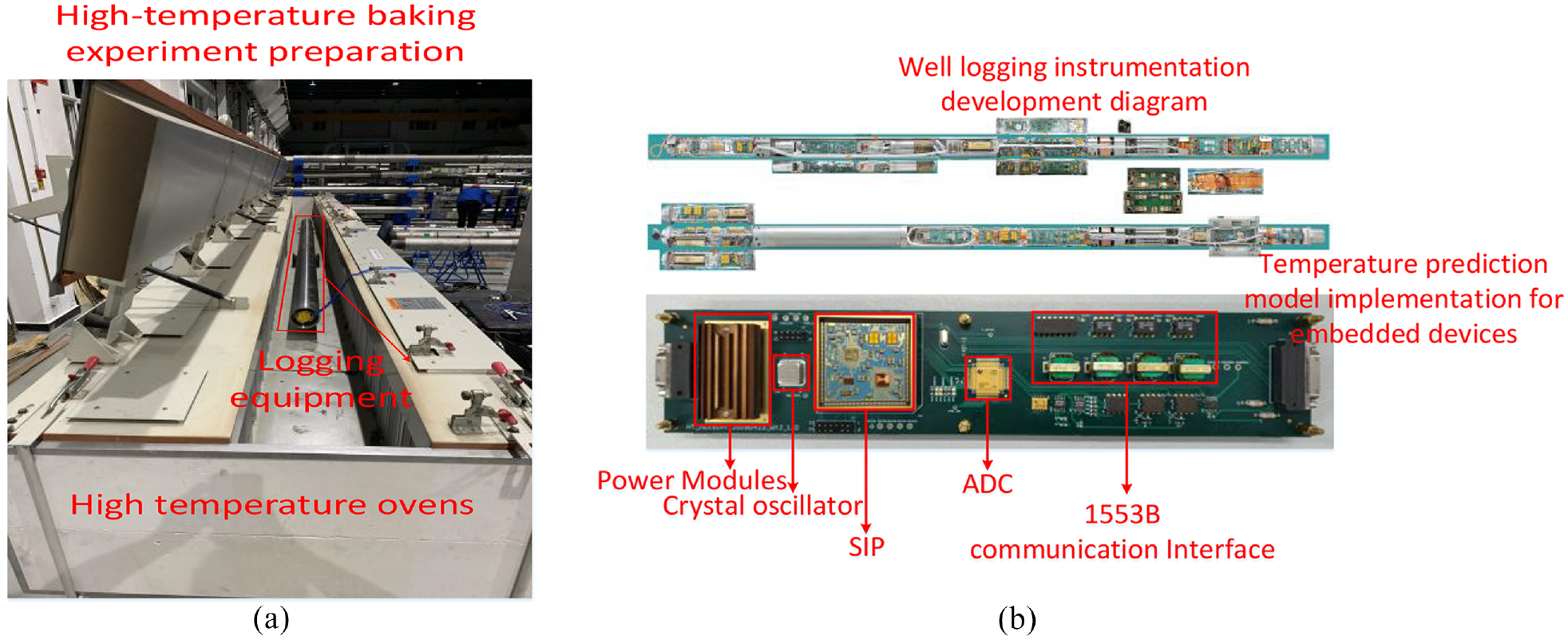
Structure of the experimental setup (a) High-temperature baking experiment preparation and (b) Well logging instrument development diagram.
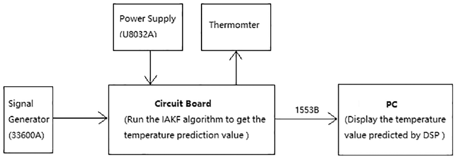
Experimental system block diagram.
To test the real-time prediction effect of the IAKF temperature prediction model implemented in the logging instrument, a high-temperature test was performed on the logging instrument containing a thermos bottle. The internal input power of this system is 73 W. The experimental environment is shown in Figure 3(a). The entire logging apparatus was located in a large oven that provided a temperature range of 51°C–260°C, manufactured by Despatch, model PTC1-40. The oven temperature was set to 200°C for 1 h, and the full test time was 650 min.
Figure 5 for the temperature curve of each temperature measurement point and ambient temperature in the oven. According to the United States Department of Defense temperature test method standards, the rate of temperature rise was controlled at about 2 °C/min. From Figure 5 ambient temperature in the temperature chamber rises first and reaches the setting 205°C by the 60th min and holds. From the figure, it can be found that the temperature change curve in each circuit is much slower relative to the rising trend of the ambient temperature, which is mainly due to the distributed phase change material used in this logging apparatus to absorb heat and play the role of thermal energy buffer. The red dotted line in the figure is the 125°C warning line. Total internal input power of the apparatus is 73 W. The upward trend in the graph for each temperature measurement point is due to the fact that the monitoring circuit is located in the thermos bottle. The differences in the temperature profiles of the circuits in the diagram are due to the different distances between each circuit and the opening of the thermos, and the different phase change materials accommodated in the distribution locations of the circuits.
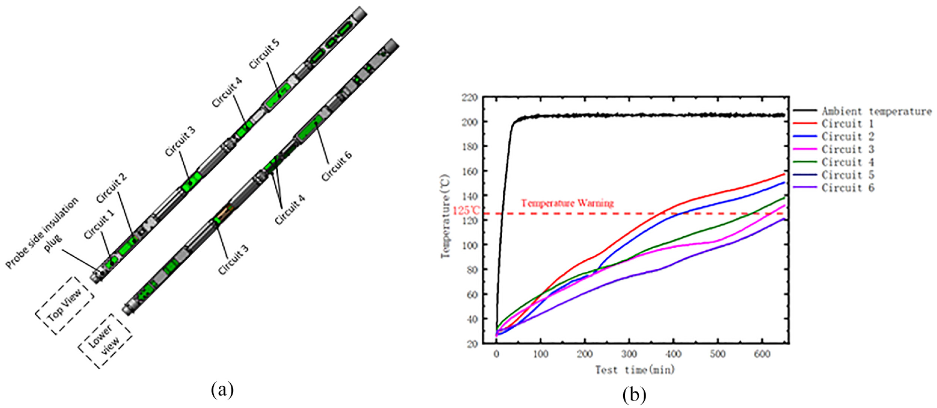
(a) Experimental circuit location and (b) temperature curves of circuits versus time.
When implementing the IAKF temperature prediction algorithm in the embedded device of the logging unit, the FPGA intermittently acquires temperature information from each temperature measurement point in 10 min steps and performs a multi-step prediction. For example, a three-step prediction is performed at 120th min, based on the previous temperature time series data as model input data, and then the temperature information is recursively obtained for 130th, 140th, and 150th min, and the temperature prediction results are uploaded to the surface information processing system via the 1553B enhanced EDIB bus using Manchester code transmission.
The temperature prediction curve of the high-temperature test of the logging apparatus and the actual measurement curve are shown in Figure 6. From the figure, we can find that the three-step prediction effect of the IAKF temperature prediction algorithm is remarkable, and the temperature prediction error of the IAKF algorithm can be quickly controlled within the effective range as time passes, and the prediction curve of each temperature measurement point is basically consistent with the actual temperature measurement curve; among them, the temperature prediction effect of the circuit 6 is best. This is mainly due to the fact that it is located in the middle of the logging apparatus, which is less affected by the heat transfer from the external environment and the phase change material distributed around it can absorb the heat in time.
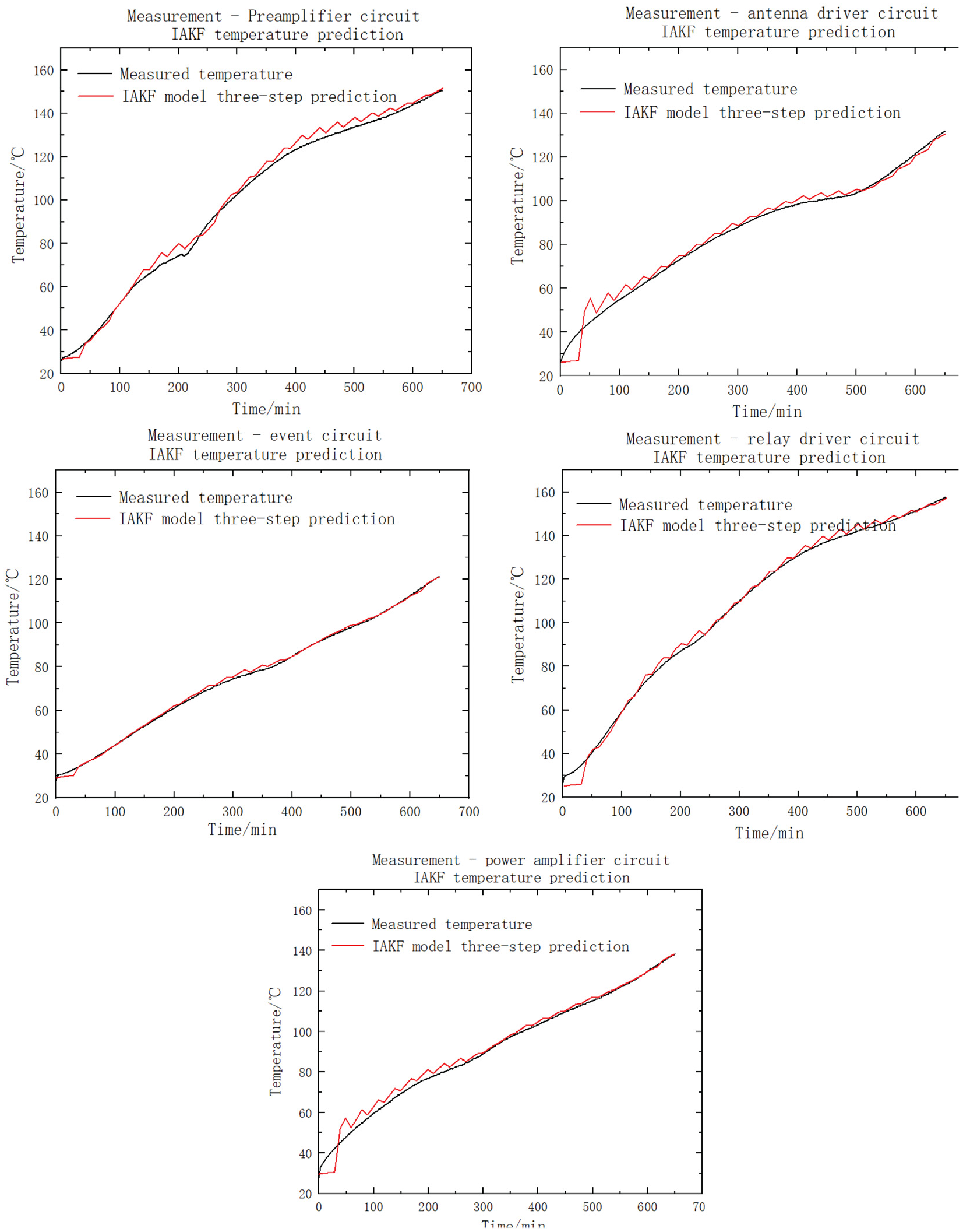
Three-step prediction effect based on IAKF temperature prediction algorithm.
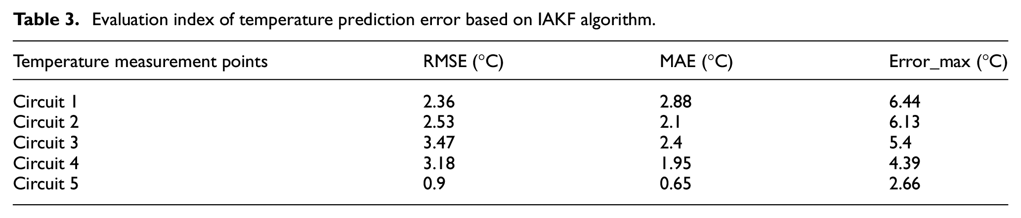
As can be seen from Table 3, the maximum temperature prediction error of the IAKF model is within 6.5°C in all three prediction steps, and the maximum relative error of measurement does not exceed 5% in the actual application requirements of engineering. In the work of the logging instrument, the worst environmental temperature faced reaches up to 200°C, so the maximum temperature prediction temperature difference of the instrument does not exceed 10°C. Therefore, the root mean square error and the mean absolute error are acceptable and meet the requirements of prediction accuracy when working with downhole logging instruments, which can be implemented in downhole embedded equipment.
Evaluation index of temperature prediction error based on IAKF algorithm.
Conclusions
An adaptive extended Kalman filter temperature prediction model is given for the problem of limited computational resources of logging instruments, which makes it difficult to perform on-site temperature prediction. The article simplifies the design of the temperature prediction algorithm and demonstrates the stability and effectiveness of the algorithm. The results of the high-temperature experiments show that the IAKF model can effectively predict the changing trend of each temperature measurement point in the apparatus in the next 30 min, and the maximum temperature prediction error is within 6.5°C. This provides a solution to effectively solve the on-site temperature prediction problem for passive thermal management of high-temperature logging apparatus.
Footnotes
Declaration of conflicting interests
The author(s) declared no potential conflicts of interest with respect to the research, authorship, and/or publication of this article.
Funding
The author(s) disclosed receipt of the following financial support for the research, authorship, and/or publication of this article: This work was partially supported by Research Fund for the National Science and Technology Major Project of the Ministry of Science and Technology of China (2017ZX05019003).