
Abstract
The aerodynamic noise emitted by a subsonic flow of dry air through an orifice plate is estimated in terms of internal sound power level and external sound pressure level (SPL) by application of the methodology described in the international standard IEC 60534-8-3. A shortcoming of the standard in defining the efficiency of the transformation of the mechanical energy of the flow into acoustic energy is discussed. Experimental evidence of the matter is also described. An alternative model employing the resolution of Reynolds Averaged Navier-Stokes equations (RANS) by means of Computational Fluid Dynamics (CFD) techniques for the calculation of the acoustic power generated by the turbulent flow through the orifice plate is applied so as to overcome the issue.
Introduction
Aerodynamic noise in flow-regulating devices (e.g. valves, flow-measuring diaphragms) is generated by the turbulent flow of a gas through the inner body of the element and it’s a well-known problem in such fields as Oil & Gas (O&G) or Heating, Ventilation and Air Conditioning (HVAC). In fact, the noise emissions so caused may reach hazardous levels for the health of the work personnel in the neighborhood of the device. Furthermore, the aerodynamically generated sound pressure field downstream of the regulator may cause structural damages to the piping system if its frequency content is close enough to the natural one of the latter. 1 High enough levels of the overall sound pressure fluctuations independent of the frequency distribution are also known to be the source of structural problems. 2
Even though the practical importance of the topic is paramount, the coexistence of many different physical phenomena (turbulence, self noise, sound transmission along and through the pipe’s walls and propagation of the acoustic pressure through the surrounding medium) make the task of predicting noise emissions by flow-control devices a highly complex one.
Interest in the discipline steadily arose since the end of the 1960s, when the advancement in the field of aeroacoustics applied to jet engines pioneered by the works of Lighthill3,4 shed a new light on the phenomenon. Due to the intrinsic difficulty of the subject, most of the early research in control flow devices has been experimental in nature. Among the earliest works one may cite the experimental campaign by Jenvey 5 on the aerodynamic noise generated by flow through simple orifice plates placed in circular ducts. In his work, Jenvey derived a relationship between the applied pressure drop across the valve and the acoustic power emitted by the orifice. He did so by a rewriting of the formulation obtained through dimensional reasoning and experimental campaigns by Lighthill for free turbulent jets, therefore assuming a quadrupole-like source for the aerodynamic noise of control devices. The theoretical results closely followed those obtained by an experimental campaign. However, Blake 6 later contested that the orifice plates employed in Jenvey’s work had too small of a hole-to-pipe diameter ratio, therefore favoring the quadrupole source linked to turbulence proper over the dipole source due to the interaction with the solid surfaces. This last observation may be of particular importance for the case of subsonic flows, as demonstrated by Nelson and Morfey. 7 In their work, the noise issuing from spoilers in rectangular ducts, commonly found in the HVAC sector, was studied in detail. In particular, the authors argued that the main contribution to noise generation is the dipole distribution caused by the exchange of a fluctuating drag force between the fluid and the orifice surface. By making the hypothesis that the fluctuating component of such force is directly proportional to the steady-state one through a generalized spectrum, they were able to compute the sound pressure level (SPL) generated by a series of rectangular spoilers of various widths. An experimental campaign validated their results. Other authors followed the lead of Nelson and Morfey’s work, demonstrating the validity of the dipole-type source for low Mach number flows.8–11
The previous review of the literature highlights the fact that the precise mechanism of sound generation by control devices is still to some degree unaccounted for. It is in this context that the International Electrotechnical Commision (IEC) 12 issued a standard, the IEC 60534-83, currently in its third revised form, which provides a method to estimate the sound production of control devices through the knowledge of their sizing coefficients and working conditions. 13 The standard draws from the body of knowledge on the subject by combining the results from the theory of Lighthill for free turbulent jets and the models of acoustic transmission through the pipe walls by Fagerlund and Chou. 14 The method has been successfully applied over the years by the valve manufacturing community. 15 However, in its development a large use of empirical factors was made. This has led to a loss of case-specific precision in favor of a more generality of the approach.
A particularly delicate matter in the standard is the definition of the efficiency of transformation of the mechanical energy of the flow into acoustic energy. In order to do so the standard makes use of a parameter, the valve correction factor for acoustical efficiency Aη. Though indicated to be varying with flow conditions, only generic constant values for given flow-control device categories (e.g. orifice plates, butterfly valves) are provided.
The present paper deals with this last issue of the IEC 60534-8-3 standard. In particular, experimental evidence from previous works of the variation of Aη is given and a literature model for the acoustic power of a turbulent region is employed combined with numerical results coming from Computational Fluid Dynamics (CFD) techniques. This allows to obtain an a posteriori estimate of the Aη coefficient, which is shown to vary with the flow conditions.
The remainder of the paper is structured into four sections. The acoustical characterization of flow-control devices provided by the IEC 60534-8-3 is first briefly described and the most important parameters defined by the standard for this purpose are introduced. Then, a sensitivity analysis of the predicted external noise on two of those parameters, that is, the Aη coefficient and the Strouhal number for peak frequency Stp, is discussed. The dependency of the former on the flow conditions according to previous experimental data is then shown. The acoustic model for the evaluation of the acoustic power from CFD numerical simulations is presented. The Aη coefficient is thus calculated for a perforated plate installed inside a pipe under different flow conditions. The results are then used for the prediction of the external noise according to the procedure provided by the standard IEC 60534-8-3. A comparison with the results obtained by employing the values of Aη suggested by the standard for orifice plates follows. Finally, conclusions about the alternative model introduced in this work are drawn.
IEC 60534-8-3 summary
The scope of the standard is the estimation of the external noise emitted by flow-control devices installed along a pipeline where a single-phase gas is flowing. In particular, the noise emissions are expressed in terms of the SPL at a point located 1 m far from the pipe’s external walls and 1 m downstream of the valve’s outlet. Its definition is:
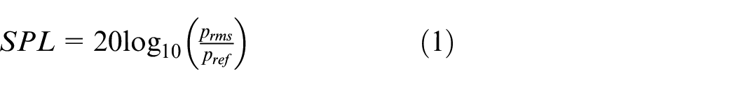
where prms is the root mean square of the pressure fluctuations and pref is a reference value of pressure corresponding to 2·10−5 Pa. The SPL is measured in A-weighted decibels or dB(A), thus taking into account the human ear’s preferred sensitivity to a particular frequency range. 13 For its application, the standard requires the description of a control device in terms of certain fluid dynamic and acoustic parameters as well as the hydraulics of the system (applied pressure differential Δp, upstream absolute pressure p1, temperature T), the flowing fluid’s properties (inlet density ρ1 and specific heat ratio γ) and the pipe’s structural properties (diameter D, thickness s, and density ρs). All hydraulic quantities are measured 2D upstream of the device and 6D downstream of it.
With regards to the fluid-dynamic characterization of the device, the standard makes use of the flow coefficient CV, the liquid pressure recovery factor FL and the valve style modifier Fd. In particular, the CV coefficient indicates the resistance opposed by the device to the flow and it is expressed in the non-I.S. units of [gpm/psi0.5]. The nondimensional FL factor is an indicator of a valve’s capability of converting kinetic energy back into pressure energy at its exit. Its values are limited to the range [0,1] and the closer to unity the less efficient the valve is at recovering kinetic energy, which is thus dissipated into turbulent kinetic energy. Finally, the non-dimensional Fd coefficient takes into account the deviation of the mean flow downstream of the valve from the benchmark case of a round jet; its value being equal to 1 for simple orifice plates and less than one for all other geometries of the flow passage area. The evaluation of these parameters is performed according to another part of the standard IEC 60534 16 and can be dealt with either through experimental or numerical procedures.
The acoustic characterization of the device is described in the standard in terms of the already mentioned nondimensional valve correction factor for acoustical efficiency Aη and the Strouhal number for peak frequency Stp. The former is involved in the expression of the efficiency of the transformation of part of the mechanical energy into acoustic energy, that is, the acoustical efficiency η. The latter is involved in computing the peak frequency of the acoustic pressure fluctuations downstream of the pipe. The standard states that these values could depend both on the geometry of the device and on the flow conditions, that is, the applied pressure differential Δp, the temperature T, the absolute upstream pressure p1. Unlike for the fluid-dynamic coefficients however, no test procedures are proposed for their evaluation, but instead constant values are listed for the most common flow-control devices available on the market.
Figure 1 summarizes the main steps of the procedure and the role played by the four mentioned parameters in the noise computation.
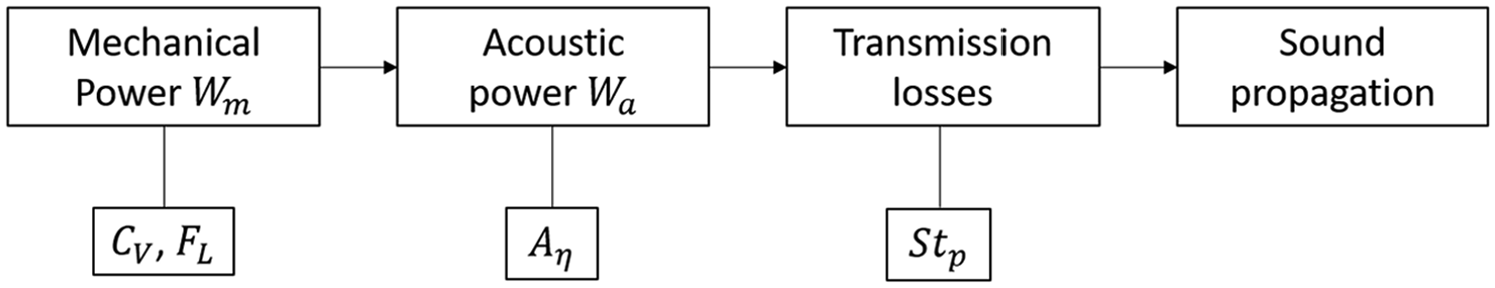
Scheme of the IEC procedure for valve aerodynamic noise prediction.
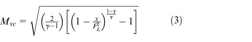
The FL and the CV are employed in the evaluation of the mechanical power Wm of the flow together with the hydraulic input data. A small portion of Wm is converted into acoustic power Wa because of turbulence: the ratio of the acoustic to mechanical power is defined as the aforementioned acoustic efficiency η = Wa/Wm. Based on the differential pressure ratio x = Δp/p1, five different regimes of noise generation are defined by the standard. The present paper is limited to regime I, whereby subsonic conditions are present both in the upstream and the downstream branches of the pipe. For such regime, the expression for the acoustic efficiency is:

where Mvc is the Mach number in the vena contracta, itself a function of FL and of the specific heats of the flowing gas
The fundamental role played by the Aη coefficient is clear, as it appears as the exponent in (2) and is therefore the most important parameter in defining the amount of mechanical energy which is radiated as sound downstream of the pipe. The transmission of sound through the pipe’s walls is dealt with by the standard through a decomposition of the noise in frequency bands, for which the filtering effect of the pipe is applied; the Stp is involved in such decomposition. Finally, the SPL at 1 m downstream of the valve and at 1 m far from the pipe is computed by assuming a cylindrical propagation of sound in the outside environment.
Parameters for acoustical characterization
As flow-control devices regulate the flow by forcing the passage of a fluid through one or multiple constrictions, the flow at the outlet can be usually described as the interaction of one or multiple closed jets. Indeed, jets are one of the most studied configurations in aeroacoustics, either freely expanded or enclosed. 17 As such, the chosen benchmark configuration for the work presented in the paper is that of a perforated plate whose axis is aligned with the pipe’s one, reported in Figure 2. The sensitivity of the predicted noise levels on the two acoustic parameters Aη and Stp is first performed.
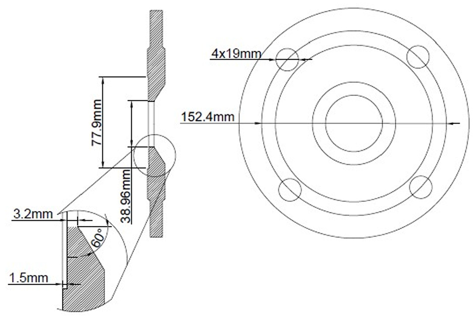
Dimensions of the ISA orifice plate. 18
The design of the tested orifice is the one described in the ISA international standard (Figure 2). 18 This was done in order to remove any uncertainty relative to the values of the fluid-dynamic parameters CV, FL, and Fd. The values of such parameters and the ones suggested by the IEC for the acoustical ones are reported in the following Table 1:
Characterizing parameters for the ISA orifice plate, from ISA and IEC 60534-8-3.
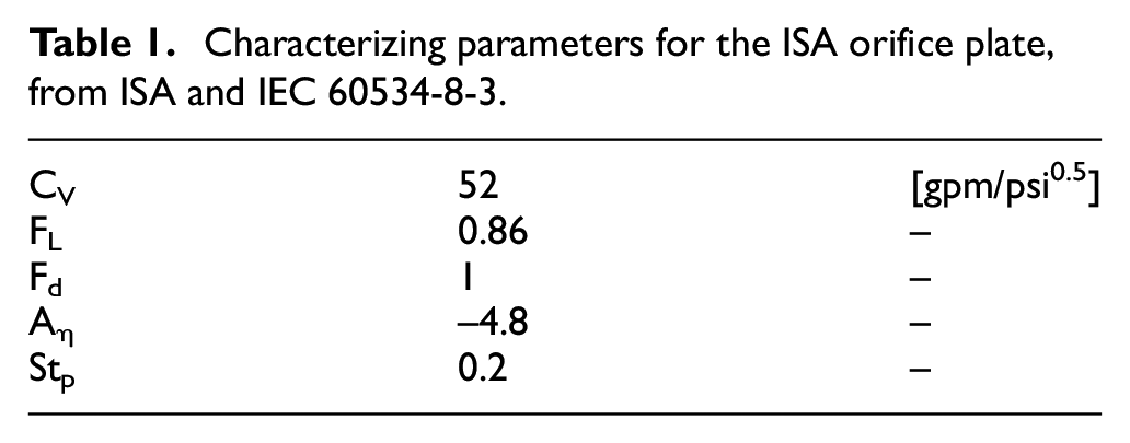
In particular, the values suggested by the IEC for Aη and Stp are those of a generic perforated plate configuration, with no regards to its design (sharp- or round-edged, number of perforations, thickness of the plate). The sensitivity analysis presented in the next section is thus finalized to the evaluation of the effect of these parameters’ uncertainty on the external noise and to the identification of the parameter which most affects the SPL prediction.
Noise sensitivity on the acoustic parameters
The influence of Aη and Stp on the SPL is investigated at varying differential pressure ratios employing for the two parameters values in the ranges found in the IEC standard and the equations (2) and (3). The calculations are conducted with constant upstream absolute pressure p1 = 5.2 barA and with a pressure drop Δp going from 0.1 bar to 1.3 bar, the latter corresponding to a jet Mach number close to 0.8. The IEC ranges for the two parameters are Aη∈ [−4.8,−3] and Stp∈ [0.19,0.3]. In Figure 3 the SPL obtained at different pressure ratios x and the variability of the results with the values of Aη and Stp are shown. In particular, the base curve (in black) is that obtained employing Aη = −4 and Stp = 0.2.
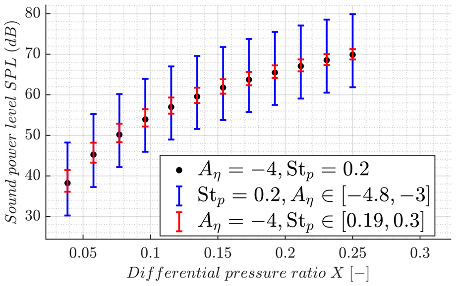
Variability of the external noise evaluated according to the IEC procedure with the acoustic parameters Aη and Stp employing (2) and (3).
The sensitivity of the SPL on the value of Aη is much greater than the one on Stp. In fact, differences of up to 18 db(A) are measured due to the different values of Aη employed, while the variation due to Stp is limited to no more than 3.6 dB(A). It can be shown that a variation on Aη of 0.1 induces a change in the predicted external noise of 1 dB. 19 Because of the major influence of the valve correction factor for acoustical efficiency on the noise, the following sections are devoted to the analysis of an acoustic model for the derivation of Aη which considers its variation with the flow conditions.
Experimental evidence of Aη dependency on flow conditions
The assumption of a constant value of the valve correction factor for acoustical efficiency Aη was shown to underestimate the actual values of SPL. In particular, Mazzaro 20 measured the SPL of a perforated plate (of a different geometry than the one subject of this paper) inside an anechoic chamber according to the prescriptions outlined in the IEC standard. The results are reported in Figure 4, which shows the measured SPL for varying x together with the estimated one using Aη = −4.8 (orifice plates) and Aη = −4 (dipole sources).
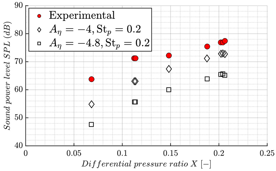
Noise prediction according to IEC with Aη = –4, Aη = –4.8 and experimental data. Figure adapted from Mazzaro. 20
The experimental data shows that the IEC underestimates the emitted noise and in particular the prediction with Aη = −4.8 is always more than 10 dB lower than the recorded SPL. As expected from the previous consideration about the influence of Aη on the SPL, the two IEC series are just shifted of 8 dB because they are computed with two Aη that differ of 0.8. It is thus possible to observe that a constant difference in the valve correction factor for acoustical efficiency returns a constant shift of the noise curves. Unlike the IEC data, the experimental results are not shifted by a constant quantity; instead, they get closer and closer to the results obtained for Aη = −4 as x increases. This is indirect evidence of the fact that the Aη factor is not constant with the flow, otherwise a constant shift with the IEC curves would have been observed.
Acoustic model for Aη estimation
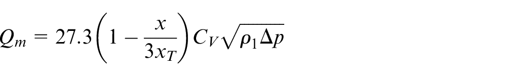
The Aη factor can be obtained by inverting (2) once the acoustic efficiency η is known. To be able to do this means having an expression for the acoustic power Wa and the mechanical power Wm, being η their ratio. The IEC formula for the mechanical power in noise generation Regime I is:
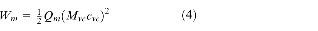
where Qm is the mass flowrate and cvc is the speed of sound in the vena contracta, for which the standard provides the formulas:
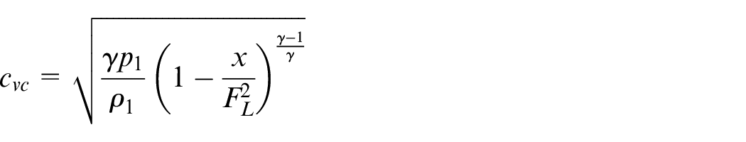
with
Since the IEC standard computes the acoustic power in terms of η and Wm, and therefore in terms of Aη, a different model for such quantity is here used. In particular, the model of Proudman for the acoustic power density P of a fluid subject to isotropic freely decaying turbulence in low Mach number flows is used. 21 On the one hand the model presents the advantage of being able to describe the noise-generation mechanism in terms of the statistics of the turbulence, that is, the turbulent kinetic energy K and the turbulent dissipation rate ε. These can be readily computed through numerical simulations solving the compressible RANS equations in the fluid domain. On the other hand however, the validity of the formulation in the case of the non-isotropic turbulence generated by control devices and the relatively high Mach numbers may be questionable. Furthermore, as the model was developed starting from Lighthill’s results for free turbulent jets, the possible dipole-nature of the noise generation mechanism is not considered. As for the assumption of freely decaying turbulence, Proudman himself questioned it stating that in such a case the turbulent energy dissipation may just be represented by the rate of introduction of energy in the flow in steady conditions. The expression for the acoustic power density is:
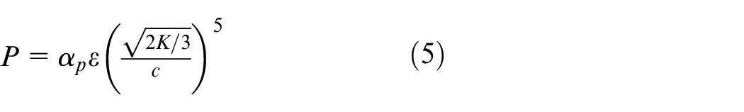
where c is the speed of sound and αP is a constant.
Different literature values for αP have been suggested in the range (0.629,13); in this paper a re-scaled model that sets it equal to 3.804 is used. 22 The total acoustic power can then be computed by integrating P over an aptly defined source region:
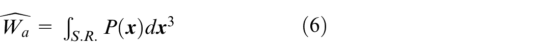
The source region (S.R.) is defined in this paper according to Mesbah 23 who considered it the flow region for which the turbulent kinetic energy K is higher than 20% of the maximum value attained. The hat is here applied to distinguish the acoustic power estimated with Proudman’s formula from the value Wa computed through the acoustical efficiency η. Inverting the resulting equation, the estimation of the valve correction factor for acoustical efficiency is obtained:
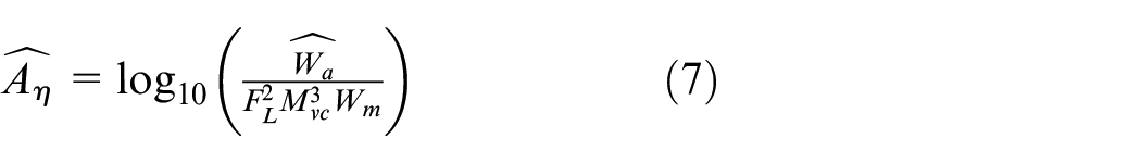
The described model for the acoustic power of the flow is applied for the computation of the
Results and discussion
The numerical acoustic power

the only way to make Wa∝U 8 is to impose:

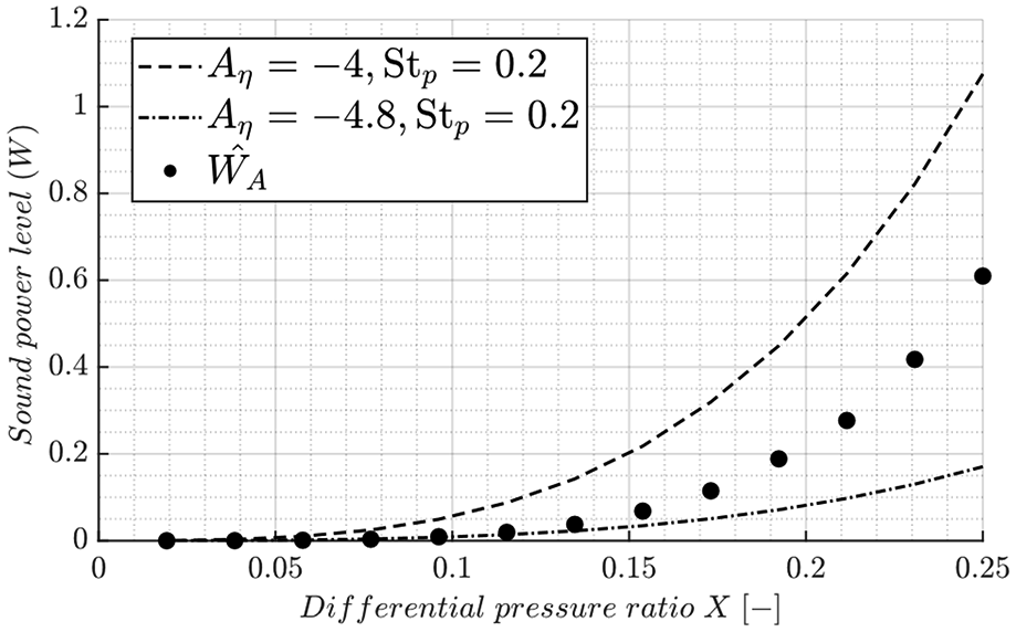
Acoustic power depending on the differential pressure ratio X evaluated with Aη = −4, Aη = −4.8 and from
This theoretical analysis is confirmed by the graphical representation in Figure 6 of the
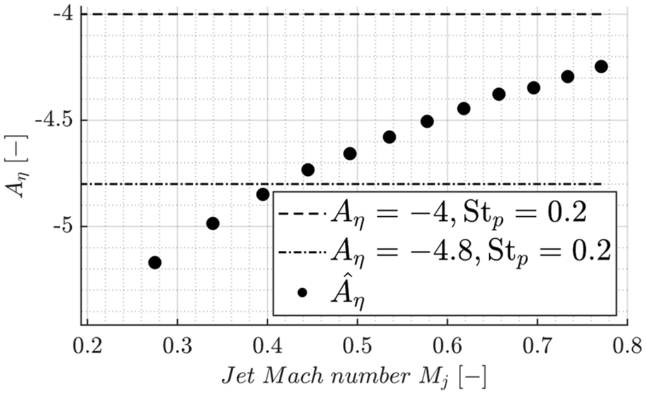
Curve of
The underestimation of Aη for low Mach numbers is an acceptable error because in these flow conditions the compressibility effects are very weak and low noise generation is expected. This is confirmed by the analysis of the external noise computed in terms of SPL with
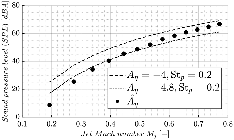
External noise in the position indicated by IEC 60534-8-3, depending on the jet Mach number: comparison of the values returned with Aη = −4, Aη = −4.8 and
Conclusions
The procedure for the estimation of the acoustical emissions of a control-flow device according to an international standard (IEC 60534-8-3) was presented. In particular, emphasis was put on the five parameters characterizing the procedure. Three of them, that is, CV, FL, and Fd, can be computed with tests, either numerical or experimental in nature, 25 proposed by the same standard. No guidelines are instead provided for the evaluation of the other two, that is, Aη and Stp, for which only constant values are tabulated for the most common valve categories on the market. A sensitivity analysis of the external noise on the latter two showed that Aη, the valve correction factor for acoustical efficiency, is the one that most affects the SPL prediction.
An alternative procedure based on a literature model for the computation of the acoustic power from CFD simulations solving the compressible RANS equations was employed for estimating Aη and predicting the emitted noise of a simple orifice subject to subsonic flow. The results showed that the obtained acoustic power lies between the values computed with the procedure suggested by the standard for a generic dipole source, Aη=−4, and for a generic perforated plate Aη=−4.8. The comparison of Wa and
Footnotes
Declaration of conflicting interests
The author(s) declared no potential conflicts of interest with respect to the research, authorship, and/or publication of this article.
Funding
The author(s) disclosed receipt of the following financial support for the research, authorship, and/or publication of this article: This project has been partly funded by Pibiviesse S.r.l, Nerviano (MI), Italy.