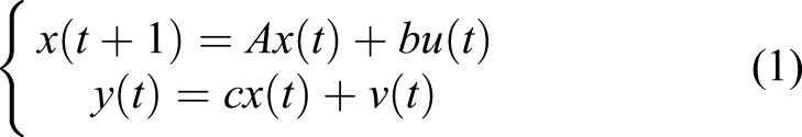
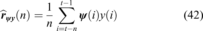
Due to the existence of system noise and unknown state variables, it is difficult to realize unbiased estimation with minimum variance for the parameter estimation of canonical state space model. This paper presents a new least squares estimator based on bias compensation principle to solve this problem, transforms canonical state space into the form suitable for the least square algorithm, introduces an augmented parameter vector and an auxiliary variable, derives parameter estimation formula based on noise compensation, realizes the unbiased estimation, and gives the specific algorithm. A simulation example is provided to verify the effectiveness of the estimator.
State space model is an effective tool to describe systems. Due to its simplicity of equations and ease of understanding, state space model has been widely used in modeling and forecasting in economic, control, biological, and other fields. However, the state space model contains both unknown state vectors and unknown parameter vectors, and the nonlinear product relationship between parameter vectors and state vectors, which makes the identification of the model very complicated.1 Therefore, the parameter estimation of the state space model has always been a research hotspot in control field. At present, the main methods to estimate the parameters of state space are subspace method,2 Kalman filter method,3,4 gradient search method,5,6 least squares method,7,8 etc.
Literature review
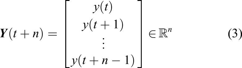
Least squares (LS) estimator is a mathematical optimization technique. The minimum variance of least squares estimator explained by Gauss Markov theorem shows that the effect of ordinary LS estimator is the best one compared with any other linear unbiased estimators. Therefore, the LS method has been widely used. However, the LS method can only use part of observed data, so it depends on the distribution of noise and the statistical properties of missing data, and it is difficult to realize unbiased estimation of parameters. An LS algorithm based on bias compensated principle (BCP) was proposed in this paper9 in view of the limitations of LS algorithm, which achieved the goal that online estimation can be realized when the order and variance of noise are unknown, and this method was widely used in parameter estimation of control systems.10–12 Kenji Ikeda et al. analyzed the asymptotic bias of recursive least squares (RLS) estimation under closed-loop conditions, and presented compensation method under the assumption that the noise is white noise.13 Wang et al. proposed a parameter and state estimation algorithm based on bias compensation for observable canonical state space systems with colored noise, which can generate unbiased parameter estimation by the bias correction term.14 For Hammerstein autoregressive moving average (ARMAX) systems with autoregressive variables, Zhang et al. proposed an RLS identification method based on the BCP.15 Wu et al. combined bias compensation technology with LS estimation algorithm with forgetting factor to estimate parameters of output error model with moving average noise,16 then, proposed an LS algorithm based on BCP for parameter estimation of MISO system under white noise.17 Mu et al. proposed a globally convergent identification algorithm, modified BCP, and gave a consistent estimation of noise variance rather than introducing auxiliary vectors.18 Jia et al. presented a unified framework based on the BCP, which introduces a nonsingular matrix and a noise-independent auxiliary vector to identify the system affected by correlated noise. Due to the rich possibility of selecting matrix and auxiliary vector, the framework has great flexibility.19
In the numerous literature studies on system parameter identification, there are not many cases of parameter identification for canonical state space model. By using hierarchical identification principle, Zhuang et al. proposed a new parameter and state estimation algorithm for canonical state space model by replacing noise term with estimation residual in an information vector and achieved good results.20 However, even if the estimated residuals take the place of the noise item, the other items of algorithm in Ref. 20 still require system noise to be known. In actual systems, the noise is usually random noise, which is very difficult to be observed. When the noise is unknown, it is difficult to estimate parameters unbiased. In this paper, LS based on BCP is used to estimate parameters of canonical state space model, so that model transformation, bias analysis, and bias compensation are carried out to obtain unbiased estimation of system parameters.
Least squares algorithm based on bias compensated principle
Parameter estimation of canonical state space model based on least squares
By LS method, unknown data can be easily obtained, and square sum of errors between obtained data and actual data is the minimum (the least variance). In this section, LS method is applied to estimate parameters of canonical state space model, and state space model in the form of equation (1) is transformed into vector functions suitable for LS method.
where, is companion matrix , and are input and output of the system, respectively, is the unobservable state vector, and is an uncorrelated random white noise with zero mean. Assume that the order is known, and when . is the system parameter matrix and parameter vector to be identified, respectively.
Since is a companion matrix and has a standard structure, that is, the first element of is 1 and the other elements are zeros, it can be seen that the model is observable canonical state space model, that is, parameters of observable canonical model are estimated.
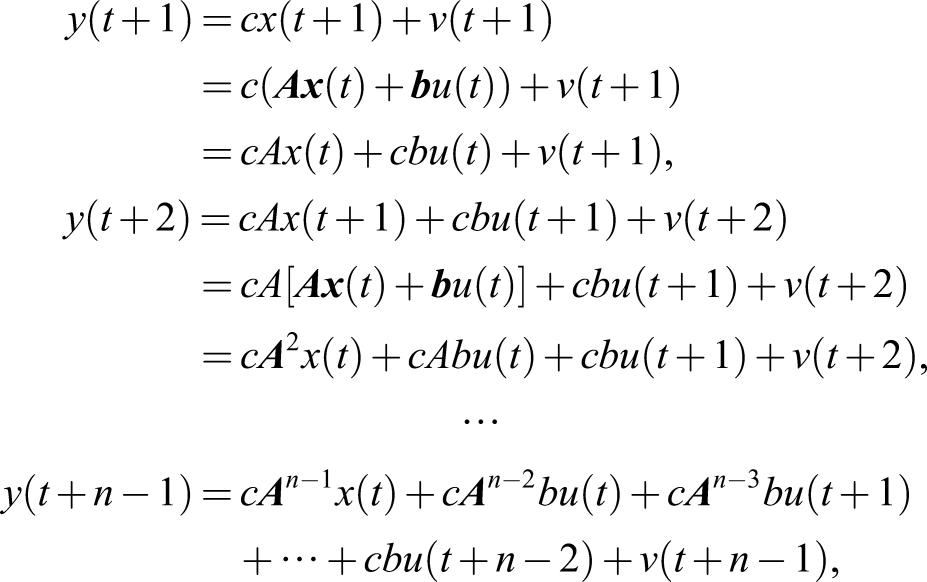
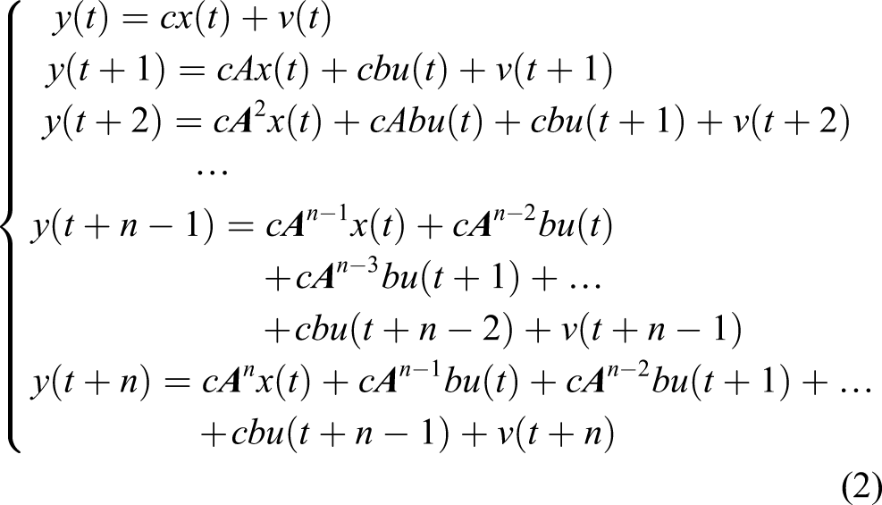
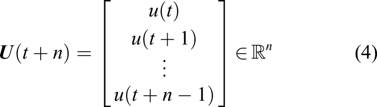
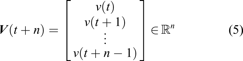
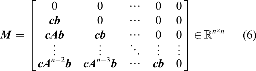
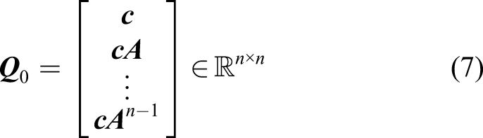
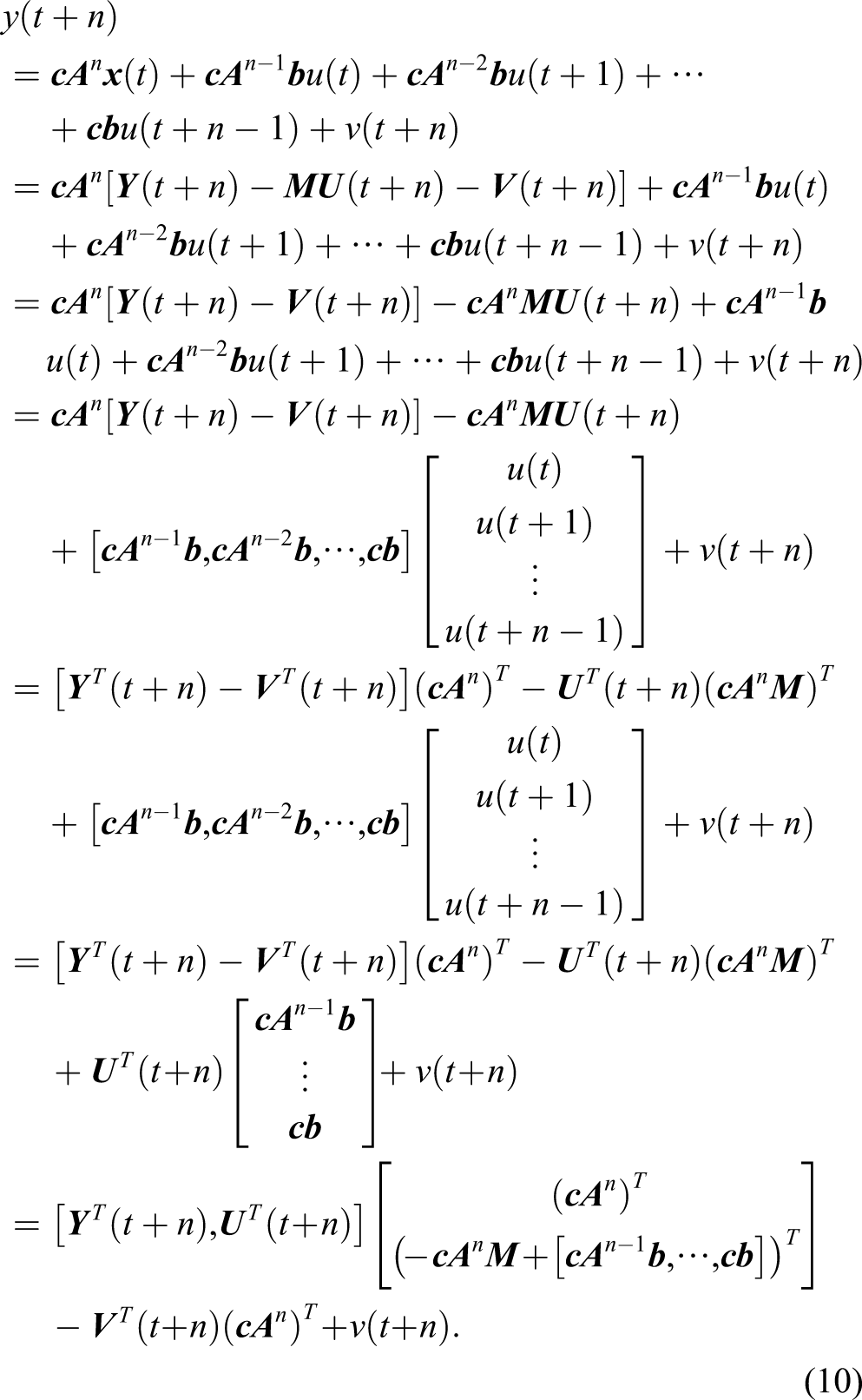
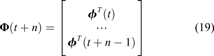
Transform the form of equation (1). The equation of vector can be obtained by deducing in equations (1) [20]:
We have
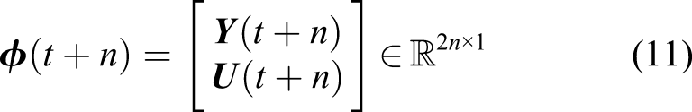
Define
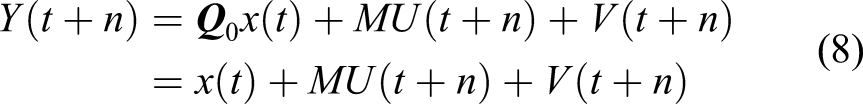
Due to the special structures of and , we have , which is an unit matrix. The first equations of equation (2) can be rewritten as (8)
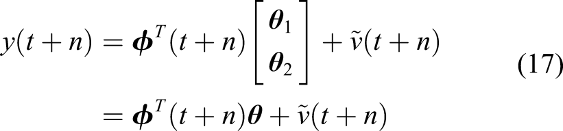
Replacing in equation (17) with yields equation (18)
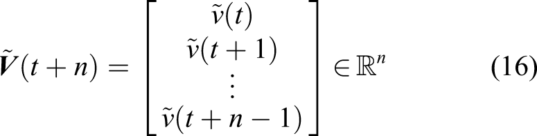
Define
So, the vector function form suitable for LS method is obtained
Replacing in equation (20) with yields equation (21)
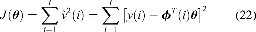
According to the principle of LS, the loss function can be defined as (22)
LS estimation can be obtained by solving the minimization of loss function
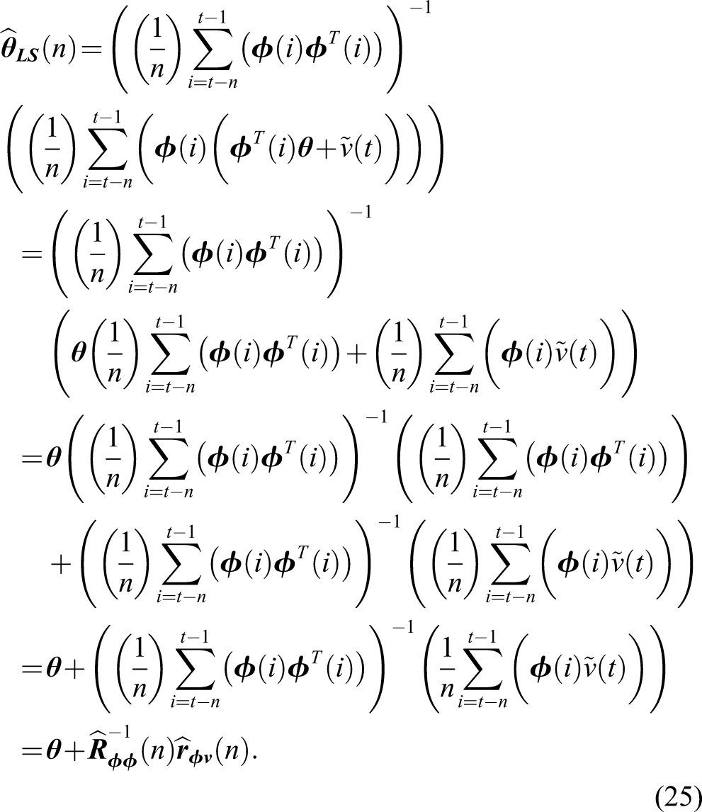
If the above equations are used to estimate directly, and then and are deduced, parameter estimation of equation (1) can be achieved. However, it can be seen from equation (14) that noise may no longer be random white noise with zero mean, so that estimation of parameters by LS method may not be the least variance, that is, unbiased estimation of parameters may not be possible. Therefore, bias compensation method will be used to eliminate the bias; the above LS estimator will be modified in order to achieve unbiased estimation.
Least squares estimator based on bias compensated principle
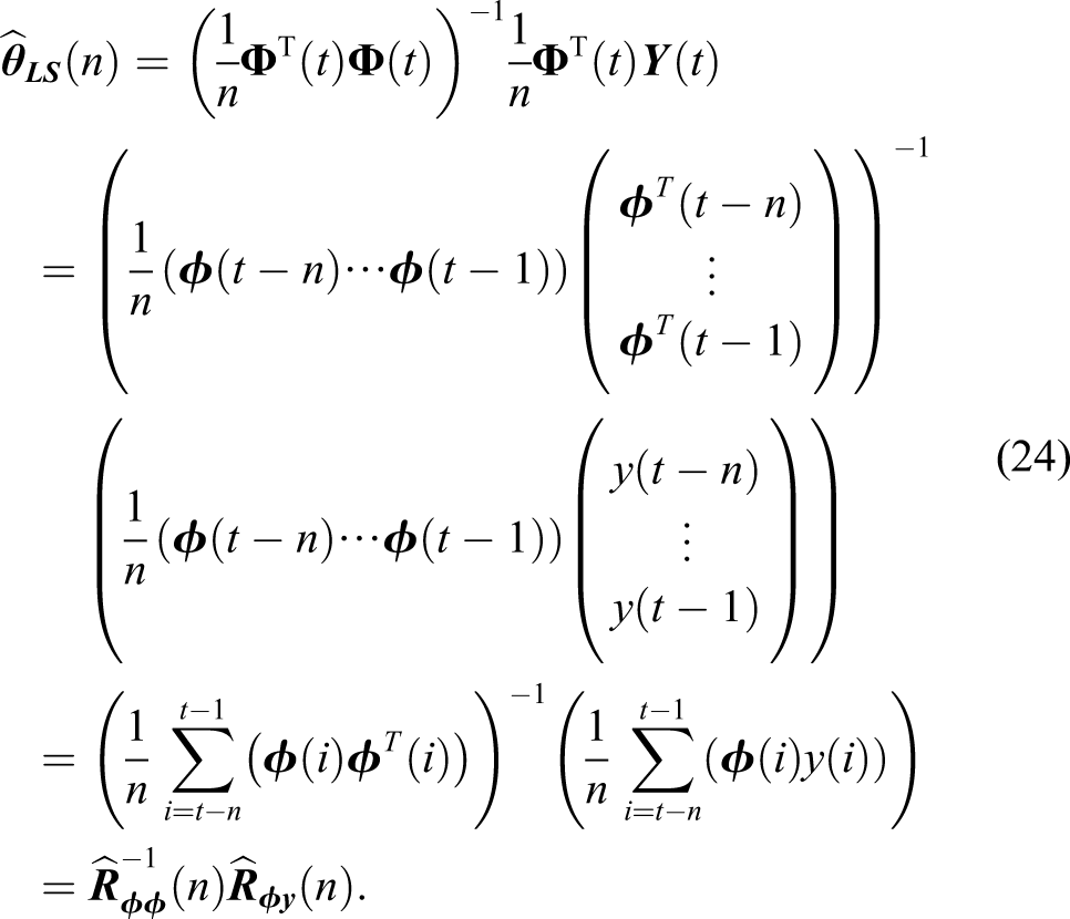
In this section, equation (21) is continuously to be deduced by LS gives (24)
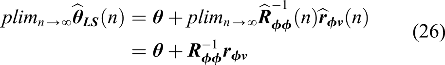
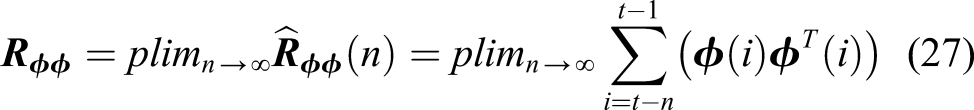
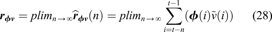
It can be seen from equation (26) that LS estimator is biased, and bias term is caused by noise. In order to eliminate the influence of bias term, equation (29) is obtained
In order to obtain an unbiased estimate of , a constant is needed to replace to compensate for the influence of bias. Assuming that system operates in an open-loop mode, it means that inputs and are not statistically relevant, then equation (28) can be rewritten as equation (30)
It can be seen from (31) that the key is to find so augmented regression vector and augmented parameter vector are introduced to satisfy , which is commonly used in BCP. It is worth noting that no matter how different the structures of and are, the calculation of is similar.19 Therefore, the method described below is universal.
Introduce an auxiliary vector which satisfies equation (32) and a nonsingular matrix
Construct an augmented regression vector and an augmented parameter vector by introducing auxiliary vector and nonsingular matrix , this step is the most important step, the selection of and makes calculation of becomes possible
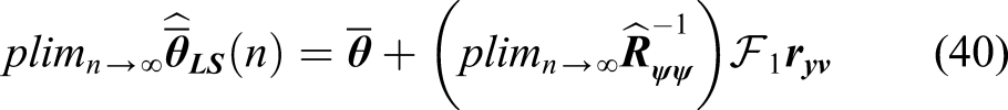
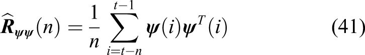
Similar to equations (24) and (26), equations (39) and (40) can be obtained in the same way
where
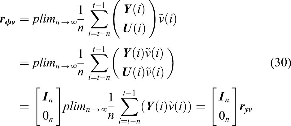
Pre-multiplying on both sides of equation (40) and using (38) yield
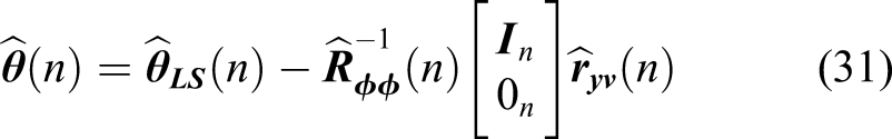
Define
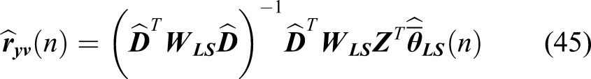
Thus, the estimation of can be determined by the weighted LS as equation (45)
where is a positive definite weighting matrix. The choice of does not affect the consistency properties of , but may have a considerable impact on the statistical accuracy of . One simple choice is .19 In the case of , if is non-singular, simply becomes as equation (46)
Similar to equations (24) and (26), equation (47) can be obtained from (40) in the same way
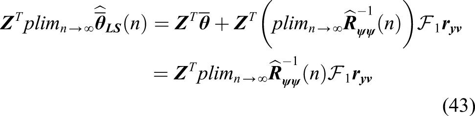
By substituting (45) into (47), consistent estimation of the augmented parameter vector can be obtained, finally, the global consistent estimation of original parameter can be obtained by equation (36) and rewritten as equation (48)
Above is the unified BCP method. Through choosing appropriately and , various BCP-based methods can be obtained to achieve a global consistent estimation of parameters.
Parameter estimation of canonical state space model based on BCP-LS
For canonical state space model, this section uses the method introduced in 2.2 to derive a specific parameter estimation algorithm.
Choose
where,weobtain
Then, can be obtained according to equation (45), and the global unbiased estimate of the parameter can be obtained by equations (47) and (48). Furthermore, parameters of the system can be estimated by input and output data. Since the relationship between parameter vector and parameters has been established in parameter estimation of canonical state space model based on least squares, the algorithm can be directly derived from algebraic operations.
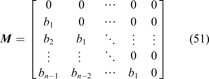
Post-multiplying by gives Observing the structure of vector to get equation (50)
The matrix in parameter estimation of canonical state space model based on least squares can be simplified by (50) as
Post-multiplying by gives
Post-multiplying by gives
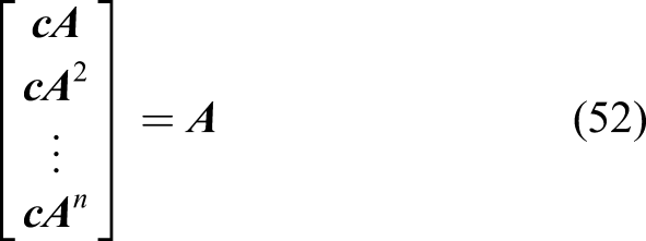
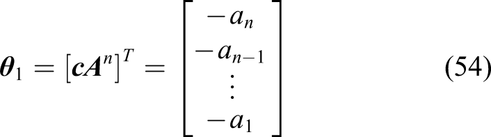
Equation (54) can be obtained according to equations (52) and (12)
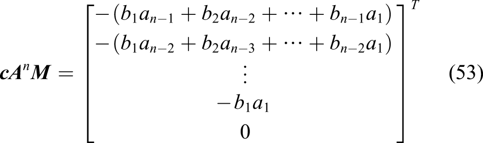
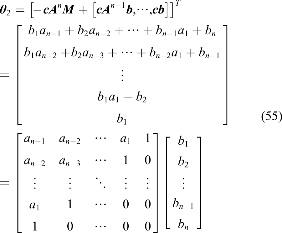
Equation (55) can be obtained according to equations (53) and (13)
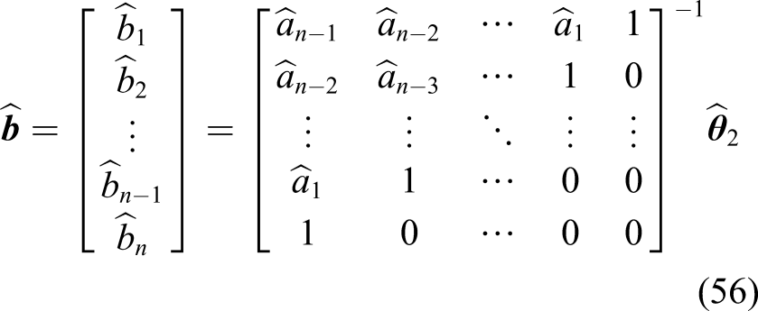
Since the estimated value of has been obtained previously, the estimated value of has been obtained, that is, the estimated value of can be obtained. Then equation (56) can be obtained due to the expression of
A consistent estimated value of can be obtained from (56). Now we have realized the global consistent unbiased estimation of parameters of canonical state space model (1).
The specific algorithm is summarized as follows:
1) Transform equation (1) into the form of according to equations (2)–(21);
2) collect the input/output data of ;
3) introduce auxiliary vector and matrix , then construct and according to equations (33) and (34);
10) calculate by equation (48), then the global consistent least squares estimation of is obtained;
11) calculate by equations (54) and (56), algorithm is end.
Simulation research
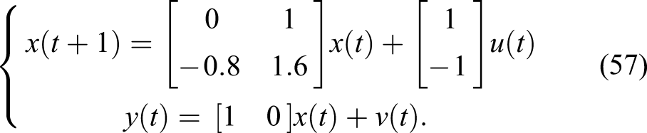
In this section, several examples of a canonical state space model are used to verify performance of presented estimator.
Example 1
For equation (57), is taken as an independent random signal sequence with zero mean and unit variance, and as a white noise sequence with zero mean and variances and , respectively. Time is represented as and parameter estimation error is calculated by , which is similar to the example in Ref. 20
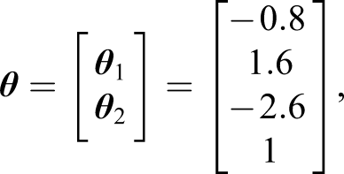
First, true value of is calculated:
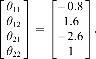
Let
Then algorithm in 2.3 is used to estimate parameters. When = 3500, the estimated value and error of are shown in Table 1:
Estimated value and error of parameter .
True value
−0.80000
1.60000
−2.60000
1.00000
Estimated value ()
−0.80039
1.59986
−2.60101
1.00049
0.0011966
Estimated value ()
−0.80079
1.60029
−2.60211
1.00149
0.0027167
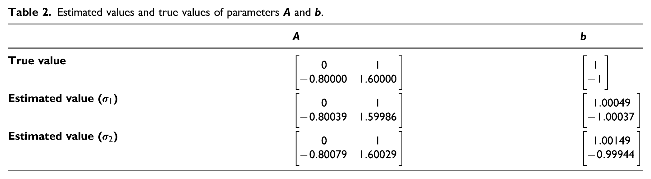
After obtaining estimated value of , the estimated values of parameters and are obtained, as shown in Table 2.
Estimated values and true values of parameters and .
True value
Estimated value ()
Estimated value ()
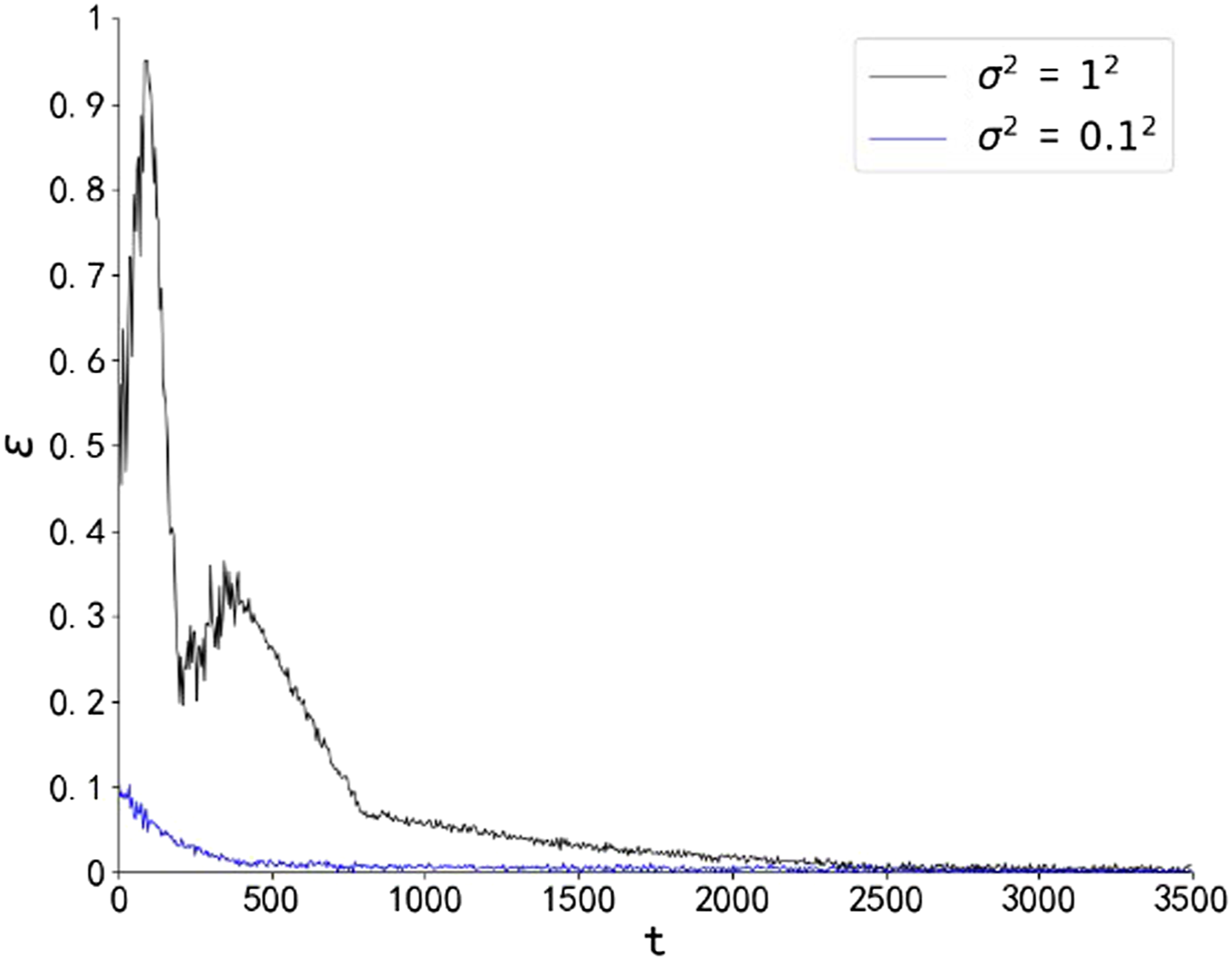
The curve of parameter estimation error with time is shown in Figure 1.
Parameter estimation error with time .
Example 2
For equations (58), in the same way, is taken as an independent random signal sequence with zero mean and unit variance, and as a white noise sequence with zero mean and variances and , respectively. Time is represented as , and parameter estimation error is calculated by
First, true value of is calculated.
Let
.
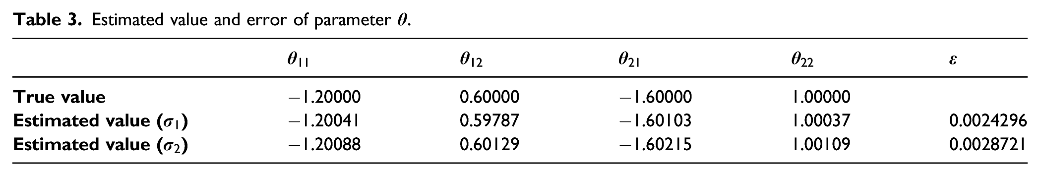
Then algorithm in 2.3 is used to estimate parameters. When = 3500, the estimated value and error of are shown in Table 3:
Estimated value and error of parameter .
True value
−1.20000
0.60000
−1.60000
1.00000
Estimated value ()
−1.20041
0.59787
−1.60103
1.00037
0.0024296
Estimated value ()
−1.20088
0.60129
−1.60215
1.00109
0.0028721
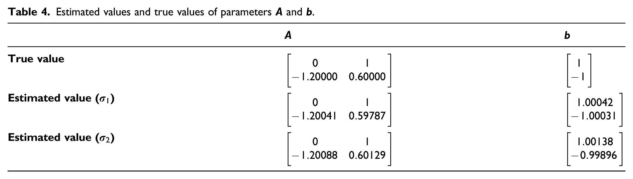
After obtaining estimated value of , the estimated values of parameters and are obtained, as shown in Table 4.
Estimated values and true values of parameters and .
True value
Estimated value ()
Estimated value ()
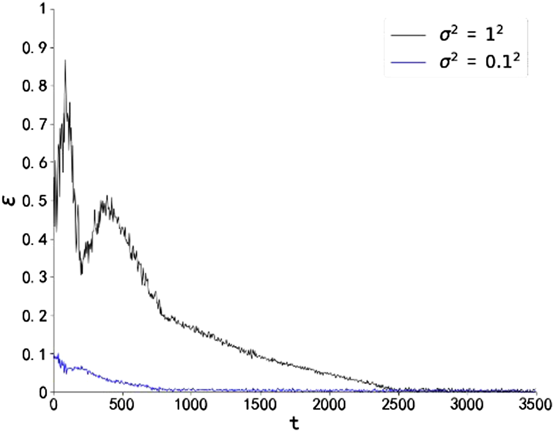
The curve of parameter estimation error with time is shown in Figure 2.
Parameter estimation error with time .
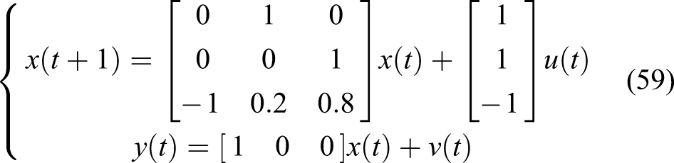
Example 3
For equation (59), in the same way, is taken as an independent random signal sequence with zero mean and unit variance, and as a white noise sequence with zero mean and variances and , respectively. Time is represented as , and parameter estimation error is calculated by .
First, true value of is calculated.
Let
.
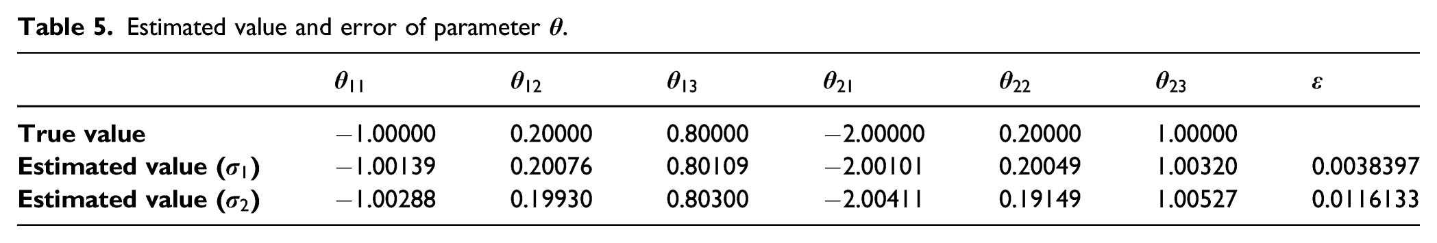
Then algorithm in 2.3 is used to estimate parameters. When = 3500, the estimated value and error of are shown in Table 5.
Estimated value and error of parameter .
True value
−1.00000
0.20000
0.80000
−2.00000
0.20000
1.00000
Estimated value ()
−1.00139
0.20076
0.80109
−2.00101
0.20049
1.00320
0.0038397
Estimated value ()
−1.00288
0.19930
0.80300
−2.00411
0.19149
1.00527
0.0116133
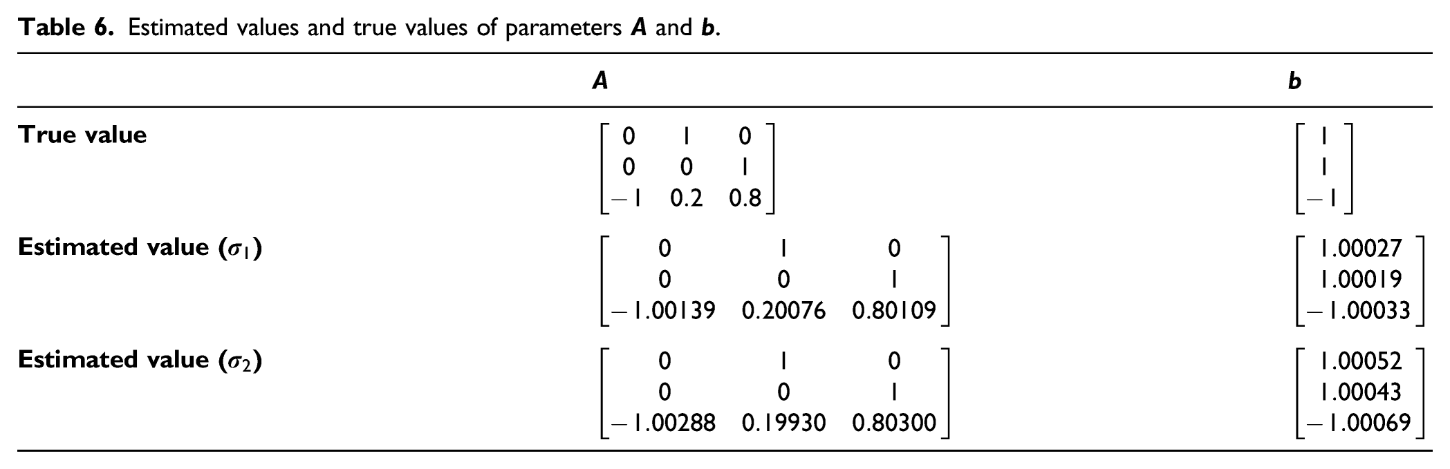
After obtaining estimated value of , the estimated values of parameters and are obtained, as shown in Table 6.
Estimated values and true values of parameters and .
True value
Estimated value ()
Estimated value ()
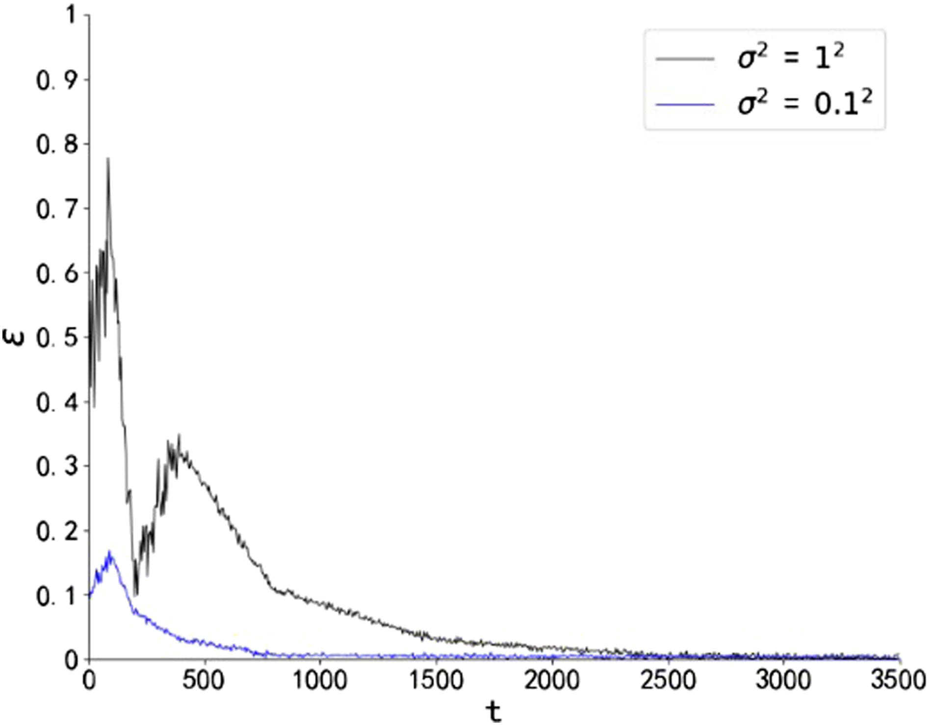
The curve of parameter estimation error with time is shown in Figure 3.
Parameter estimation error with time .
It can be seen from the three examples and Tables 1, 2, 3, 4, 5, and 6 that estimation error of parameters increases with the increase of noise, but it is still acceptable, so that the accuracy of estimator is relatively high. It is easy to see from Figures 1, 2, and 3 that the estimation error of parameter decreases with the increase of time, and the smaller the noise variance is, the faster the convergence speed of error curve is. The error will fluctuate greatly when noise variance and , but with the increase of time , it will show a downward trend, and finally achieve satisfactory results.
Conclusion
In this paper, an LS algorithm based on BCP is presented for parameter estimation of canonical state space model and a satisfactory result is achieved. The canonical state space model is transformed into vector function form suitable for LS algorithm, and then, augmented vector and auxiliary variable are introduced to realize unbiased estimation based on noise compensation; finally, the effectiveness of the estimator is verified by an example. This method of parameter estimation is universally useful, which can be extended to parameter estimation of other systems with noise, for example, parameter estimation of closed-loop system can be realized by selecting different augmented vectors, this is also our future research work. Therefore, the method presented in our paper has widespread application and practical significance.
Footnotes
Acknowledgements
Special acknowledgement to Automated Systems & Soft Computing Lab (ASSCL), Prince Sultan University, Riyadh, Saudi Arabia.
Declaration of conflicting interests
The author(s) declared no potential conflicts of interest with respect to the research, authorship, and/or publication of this article.
Funding
The author(s) received no financial support for the research, authorship, and/or publication of this article.
ORCID iDs
Ibraheem K. Ibraheem
Amjad J. Humaidi
Ahmad Taher Azar
References
1.
MaXDingF. Standard state space system identification method. J Nanjing Univ Information Technology: Nat Sci Edition2014; 6: 481–504.
2.
JuilletFSchmidPJHuerreP. Control of amplifier flows using subspace identification techniques. J Fluid Mech2013; 725: 522–565.
3.
MaXDingF. Gradient-based parameter identification algorithms for observer canonical state space systems using state estimates. Circuits, Systems, Signal Process2015; 34(5): 1697–1709.
4.
VarshneyDBhushanMPatwardhanSC. State and parameter estimation using extended kitanidis kalman filter. J Process Control2019; 76: 98–111.
5.
ZhangXDingFAlsaadiFE, et al.Recursive parameter identification of the dynamical models for bilinear state space systems. Nonlinear Dyn2017.
6.
XuehaiWFengD. Recursive parameter and state estimation for an input nonlinear state space system using the hierarchical identification principle. Signal Process2015; 117: 208–218.
7.
KrzysztofOKlaudiaD. New parameter identification method for the fractional order, state space model of heat transfer process. In: Conference on Automation. Cham, Switzerland: Springer; 2018.
8.
Wei Xing ZhengWX. On a least-squares-based algorithm for identification of stochastic linear systems. IEEE Trans Signal Process1998; 46(6): 1631–1638.
9.
SagaraSWadaK. On-line modified least-squares parameter estimation of linear discrete dynamic systems. Int J Control1977; 25(3): 329–343.
10.
StoicaPSöderströmT. Bias correction in least-squares identification. Int J Control1982; 35: 449–457.
11.
ZhangYLieTTSohCB. Consistent parameter estimation of systems disturbed by correlated noise. IEE Proc - Control Theor Appl1997; 144: 40–44.
12.
StoicaPSimonyteVSoderstromT. Study of a bias-free least squares parameter estimator. IEE Proc - Control Theor Appl1995; 142: 1–6.
13.
KenjiIYoshioMTakaoS. Bias compensation of recursive least squares estimate in closed loop environment. SICE J ControlMeasurement. and System Integration2008.
14.
WangXDingFLiuQ, et al.The bias compensation based parameter and state estimation for observability canonical state-space models with colored noise. Algorithms2018; 11(11).
15.
ZhangBMaoZ. Bias compensation principle based recursive least squares identification method for hammerstein nonlinear systems. J Franklin Inst2016: 1340–1355.
16.
WuAGQianYYWuWJ. Bias compensation-based recursive least-squares estimation with forgetting factors for output error moving average systems. Iet Signal Process2013; 8(5): 483–494.
17.
WuAGQiWNDongRQBias compensation based recursive least-squares identification algorithm for MISO system with input and output noises. In Proceedings of the 2017 IEEE 11th Asian Control Conference (ASCC), Gold Coast, QLD, 17-20 December 2017; pp. 812–816.
18.
MuBBaiE-WZhengWX, et al.A globally consistent nonlinear least squares estimator for identification of nonlinear rational systems. Automatica2017; 77: 322–335.
19.
JiaL-JTaoRKanaeS, et al.A unified framework for bias compensation based methods in correlated noise case. IEEE Trans Automatic Control2011; 56(3): 625–629.
20.
ZhuangLPanFDingF. Parameter and state estimation algorithm for single-input single-output linear systems using the canonical state space models. Appl Math Model2012; 36(8): 3454–3463.