Sage Journals: Discover world-class research

Abstract

In the past, there have been many inconsistent attempts to describe the bandwidth of dynamic systems. Similar definitions of bandwidth have been extended to describe not only the closed-loop bandwidth of feedback control systems but also the frequency at which usefulness of feedback is lost. In this work, we propose and explain the need for a new precise measure for bandwidth that could be used to describe the cut-off frequency at which the feedback control system’s usefulness is no longer advantageous. The tools of neoclassical control are used to define this new measure of bandwidth as the frequency at which the feedback controller ceases to affect the response. This measure is then applied to two example cases to demonstrate its use.

Keywords

bandwidth feedback control Youla parameterization

Introduction

A somewhat slippery term in the control literature is that of bandwidth-“slippery” because the definition is not given in a consistent and precise manner (if it is given at all) and the meaning and use of the term is somewhat vague. The term is very useful and many attempts have been made to describe it.

The idea is to convey an estimate of the length of a frequency range which is important on the Bode-magnitude curve of some dynamic system. That is, a qualitative definition of bandwidth is the frequency range over which control is effective.¹ This length is, roughly speaking, proportional to the speed at which the system responds to, say, the unit step input.

Of course, in the past, experts tried to provide a precise mathematical meaning to bandwidth where the following fundamental theorem is proved,²

Δ ω \times Δ t > \frac{1}{4}

(1)

where Δω denotes the bandwidth and Δt denotes the effective duration of a transient. This theorem clearly shows that the duration of a transient is reduced by increasing the bandwidth. However, as is obvious, this definition only provides a lower bound to the bandwidth.

Other descriptions for bandwidth include: The bandwidth is that range of positive frequency bounded by those frequencies where the Bode-magnitude falls to 3 dB below the maximum magnitude. Sometimes, 6 dB or even 12 dB are used instead and so it was referred to the –3 dB or to the -6 dB bandwidth. Additionally, only positive frequencies are used in this convention so that for the common case where the Bode diagram is monotonically decreasing, the bandwidth is taken to lie from the zero frequency to the –3 dB (or the –6 dB) frequency.

Other sources still describe the bandwidth as the span of frequencies over which a sinusoid can be tracked in a satisfactory manner.^3,4 Here, bandwidth is quantitatively defined as the largest frequency before the complementary sensitivity function drops to –3 dB.^3,4 However, rather than complementary sensitivity, other sources may instead use sensitivity^1,5 or even the crossover frequency (the frequency where the open-loop transfer function crosses 0 dB) as an approximation for bandwidth.¹

The relationship of bandwidth to speed of response is also established for both first and second-order dynamics systems. Consider the first-order system whose Bode modulus is described by

M (ω) = \frac{1}{\sqrt{1 + {(τ ω)}^{2}}}

(2)

where τ is the system time constant. Clearly, the − 3 dB bandwidth (the

1 / \sqrt{2}

frequency) is

ω_{B} = \frac{1}{τ}

(3)

Higher bandwidth corresponds to a smaller τ and a faster system response to, say, step inputs.

Next, consider the quadratic factor whose Bode modulus is

M (ω) = \frac{ω_{n}^{2}}{\sqrt{{(ω_{n}^{2} - ω^{2})}^{2} + 4 ζ^{2} ω_{n}^{2} ω^{2}}},

(4)

where ω_n is the undamped natural frequency and ζ is the damping ratio. A formula for bandwidth as a function of undamped natural frequency and damping ratio can be derived,⁶ but it turns out to be overly complex for most purposes. It is instead easier to consider the high-frequency asymptote instead. This asymptote is obtained by setting the condition ω ≫ ω_n to obtain

M (ω) \approx {(\frac{ω_{n}}{ω})}^{2}

(5)

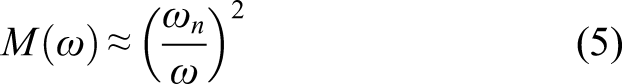
This approximation drops to the − 6 dB value at

ω_{B} = \sqrt{2} \times ω_{n}

(6)

Given the relationships between rise and settling times with the damping ratio, it follows that at a fixed value of damping ratio, the rise and settling times diminish as bandwidth is increased.

In all this development, the bandwidth is related to the system response time and not given in a consistent and precise manner. In addition, use of a bandwidth to characterize the speed of the response of dynamic systems to step inputs could at times be misleading, for example the case where the dynamic system is an integrator. In addition, when higher than second-order dynamic systems are considered, all these definitions of bandwidth become impractical unless these higher order systems could be approximated by a second-order system.

These similar definitions of bandwidth have been extended to characterize the speed of response of feedback control systems, however they have not been used to characterize by the frequency range at which feedback control is effective. Therefore, this study proposes a new measure of bandwidth as the frequency at which the feedback control system loses its usefulness, a metric that may be very useful for feedback control designers. In this work, we will show that this measure has a precise definition and that this measure could either be used as a new way to look at the feedback control bandwidth or as a precise way to characterize a cut-off frequency at which a transition from feedback to no feedback is made. Next, we use the machinery of neoclassical feedback control development^7,8 to define this measure in terms of the closed-loop feedback system transfer function. This will be a novel method of describing bandwidth that directly relates bandwidth to the frequency range of control effectiveness, rather than through indirect definitions like described earlier in this introduction.

Information as a precise measure of bandwidth

Neoclassical feedback control

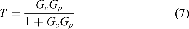
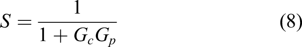
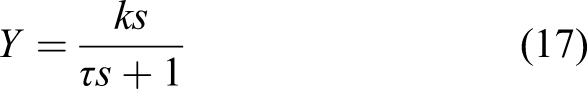
In neoclassical feedback control design, three closed-loop transfer functions are shaped in the frequency domain to meet both the performance and robustness criteria. (Note that this paper does not itself address control system robustness and sensitivity; the reader is directed to other literature^7–12 for this matter.) The closed-loop transfer functions consist of complimentary sensitivity T, sensitivity S, and Youla parameter Y. Given the feedback control loop in Figure 1, these closed-loop transfer functions can be written as

T = \frac{G_{c} G_{p}}{1 + G_{c} G_{p}}

(7)

S = \frac{1}{1 + G_{c} G_{p}}

(8)

Y = \frac{G_{c}}{1 + G_{c} G_{p}}

(9)

where, from above, we can write T = YG_p and S = 1 − YG_p.

Figure 1.

Feedback control loop.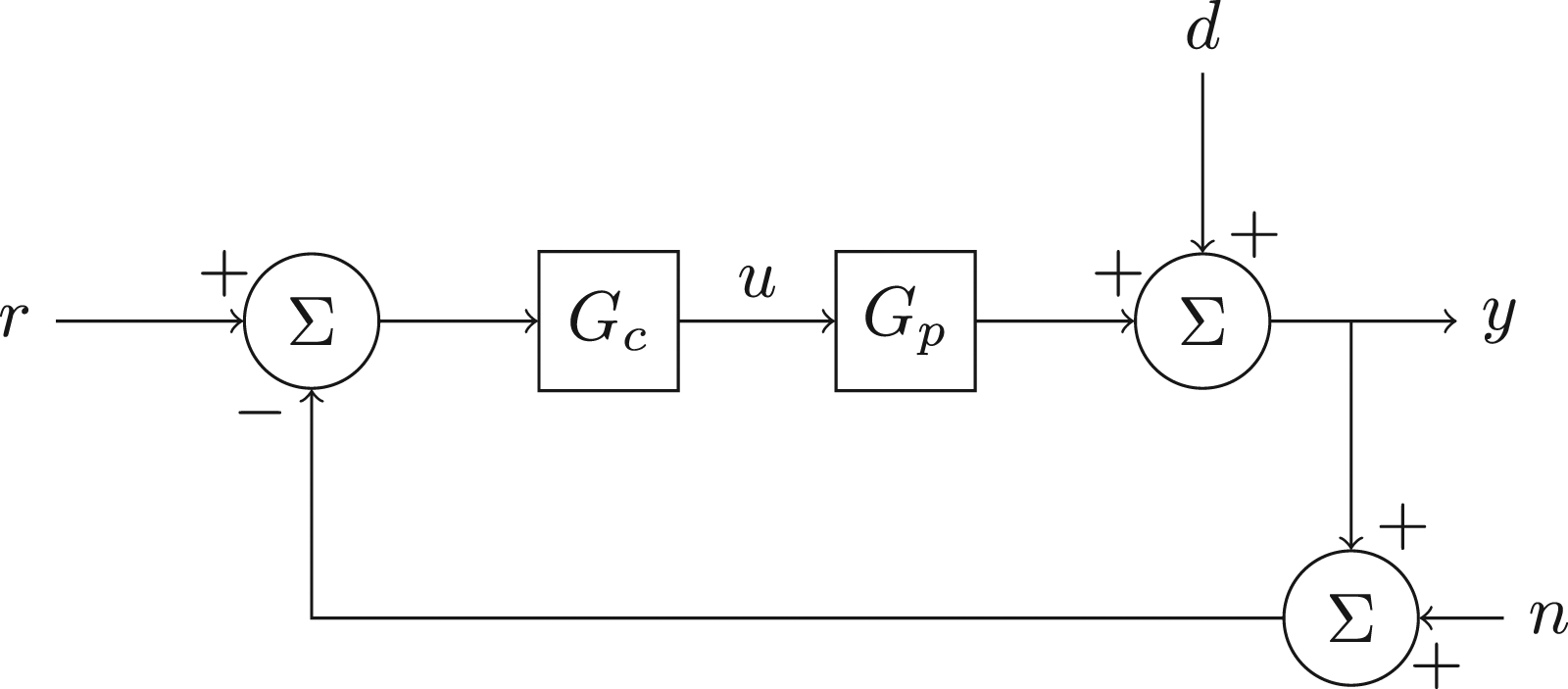

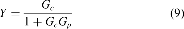
To consider the system bandwidth, these closed-loop transfer functions must all be stable. For the remainder of this section, it will be assumed that G_c has been designed in such a way to produce stable closed-loop transfer functions T, S, and Y.

Defining a measure to characterize the usefulness of feedback

In Figure 1, signal y is measured and fed back. It is known that the act of measurement introduces noise (sensor noise) to the feedback loop, and it turns out that sensor noise, due to typical sensor construction, is a high frequency phenomenon and is considered as high frequency uncertainty. In addition to sensor noise, dynamic system models cannot be modeled perfectly, meaning that in the frequency domain, dynamic models have a limited frequency range in which they can accurately represent reality. The model accuracy is therefore in the low frequency range, hence, these models introduce high frequency uncertainty (known as unstructured model uncertainty) into the feedback loop. Due to these high frequency uncertainties (sensor and unstructured model uncertainties), we are forced to abandon the feedback control loop at particular frequency. It is very interesting to notice that the act of measurement is what gives meaning to the feedback loop and the same act results in abandoning this control loop!

The closed-loop control system bandwidth (ω_B) is utilized to specify the frequency transition from feedback to no feedback, in addition to describing the closed-loop system speed of response. Interestingly enough, the definition of this closed-loop bandwidth is exactly the same as what is provided in the previous section. We argue in this work that the use of ω_B to specify the frequency transition from feedback to no feedback could be very conservative. In fact, we specify a new frequency called (ω_BC) to differentiate this new frequency from the traditional closed-loop system bandwidth, ω_B, such as those given in .equations (3) and (6) We will provide an exact computation of this frequency to illustrate the transition from feedback to no feedback when designing feedback control systems.

Computation of new bandwidth

The frequency at which a transition from feedback to no feedback (ω_BC) is computed by the use of following theorem.

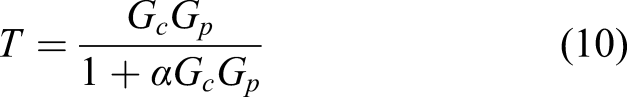
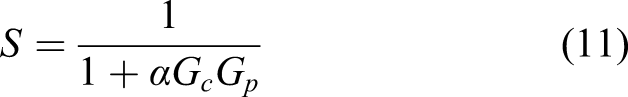
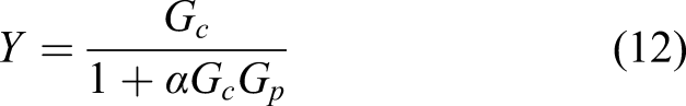
Theorem The frequency, ω_BC, at which a transition from feedback to no feedback is made, is computed using the following three closed-loop transfer functions

T = \frac{G_{c} G_{p}}{1 + α G_{c} G_{p}}

(10)

S = \frac{1}{1 + α G_{c} G_{p}}

(11)

Y = \frac{G_{c}}{1 + α G_{c} G_{p}}

(12)

where α is selected to approach from 1 (usual feedback) to 0 (no feedback).

Proof

Let’s start by the following feedback control loop given in Figure 2 below.

Figure 2.

Feedback control loop with α block.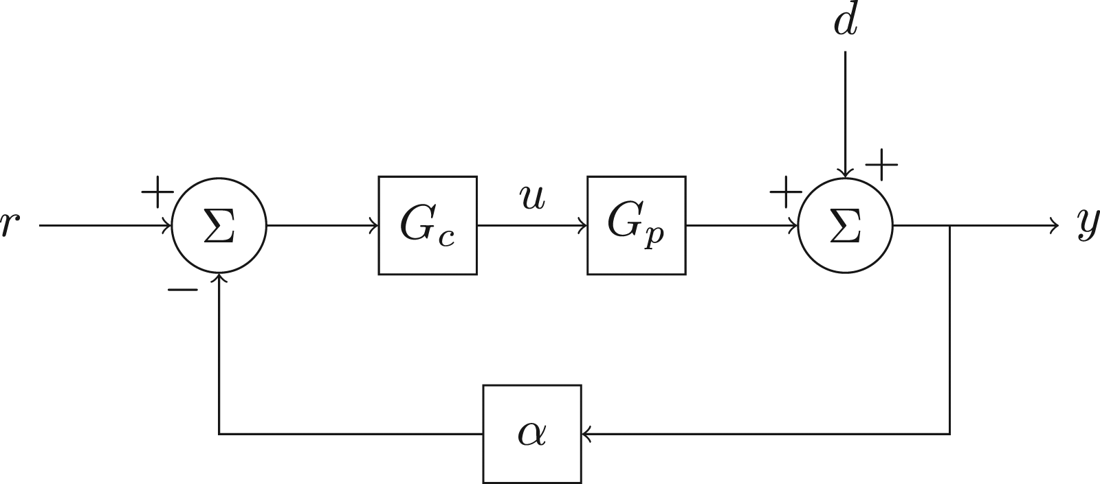

When α → 1, we have our usual feedback control system. However, when α → 0 then, obviously, there is no information that is fed back. When α → 0, the magnitudes of complimentary sensitivity and sensitivity transfer functions are given by

| T | \to | L |

(13)

| S | \to 1

(14)

where L is the open loop return ratio and is equal to G_cG_p. For computation of Youla, we use Figure 3 below. Given Figure 3, when α → 0, we have.

| Y | \to | G_{c} |

(15)

Figure 3.

Youla in Feedback Control Loop with α block.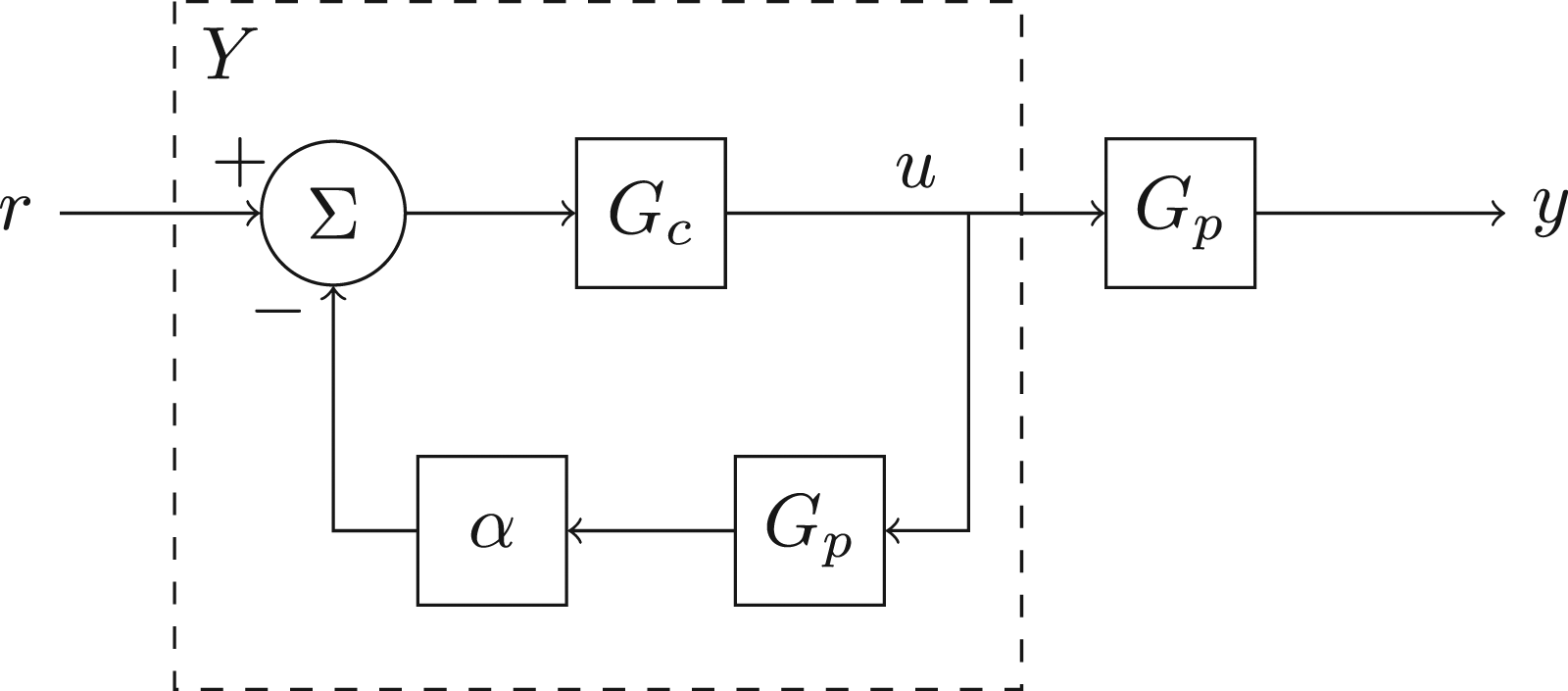

Therefore, as α → 0,

\begin{array}{l} | T | \to | L | \\ | S | \to 1 \\ | Y | \to | G_{c} | \end{array}

To show that α → 0 results in ω → ω_BC, it suffices to look at the usual feedback when α → 1 and to know that at some high frequency, |G_cG_p| ≪ 1. Then, this result is apparent from the three closed-loop transfer functions computed in equations (13)–(15).

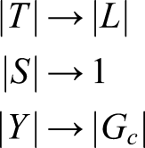
These transitions, |T| → |L|, |S| → 1, and Y → |G_c|, are known to happen at some high frequency due to forcing the magnitude of the open loop ratio |L| to be small at high frequencies. It is then interesting to see that these transitions are directly related to feedback information constant α. With the use of this constant, one can then compute the frequency ω_BC at which the benefits of feedback are lost.

Examples

In this section, we present two simple examples to illustrate the application of the proposed measure or so-called neoclassical bandwidth. It is important to note that this measure equivalently applies to more complex Single Input Single Output (SISO) and Multiple Inputs Multiple Outputs (MIMO) cases.¹³

We can write a simple MATLAB function to compute this bandwidth for a specified value of α that utilizes MATLAB’s existing ability to evaluate frequency responses. In other words, it computes the frequency at which the Youla frequency response reaches a specified percent of its final value. Effectively, this is finding when the sensitivity transfer function S settles to within a specified error bound around 0 dB. This function is given as follows:

function w_BC = NeoClassicalBW(S, alpha)

%NEOCLASSICALBW returns the systems’s

% neoclassical measure of bandwidth.

% w_BC = NEOCLASSICALBW(S, alpha)

% returns the neoclassical bandwidth

% for the given sensitivity transfer

% function S and the specified cutoff

% value of alpha. Alpha must be

% 0 < alpha < 1.

upper = 1 + alpha;

lower = 1 − alpha;

[mag,∼,w] = bode(S);

isBounded = or(mag>upper, mag<lower);

index = find(isBounded,1,‘last’);

w_BC = w(index);

end

Greater care could be taken to obtain a more precise measurement for the neoclassical bandwidth, but for the sake of these examples, the above function will suffice. It should be noted that this measure of bandwidth does not add any substantial computational complexity to the controller design process: the largest computational burden comes from finding the magnitude response of the sensitivity transfer function. However, finding this magnitude response is already a standard step in analyzing a control system design.

We can now consider two example applications. Note that goal of these examples is only to demonstrate the application and measurement of the neoclassical bandwidth, rather than to formulate a controller that meets particular design considerations.

Example 1 In this example, we examine the “Interpolation Constraints” and the consequences of violating these constraints in feedback design. Consider a force F(t) applied to a mass to control velocity, as shown in Figure 4.

\frac{\hat{v}}{\hat{u}} = \frac{1}{m s} \Rightarrow BIBO Unstable where \hat{u} = F (t)

(16)

We will examine a Youla parameter that cancels the dynamics of the mass but does not inherently meet the interpolation condition.

Y = \frac{k s}{τ s + 1}

(17)

Figure 4.

Single mass system with force input and velocity output.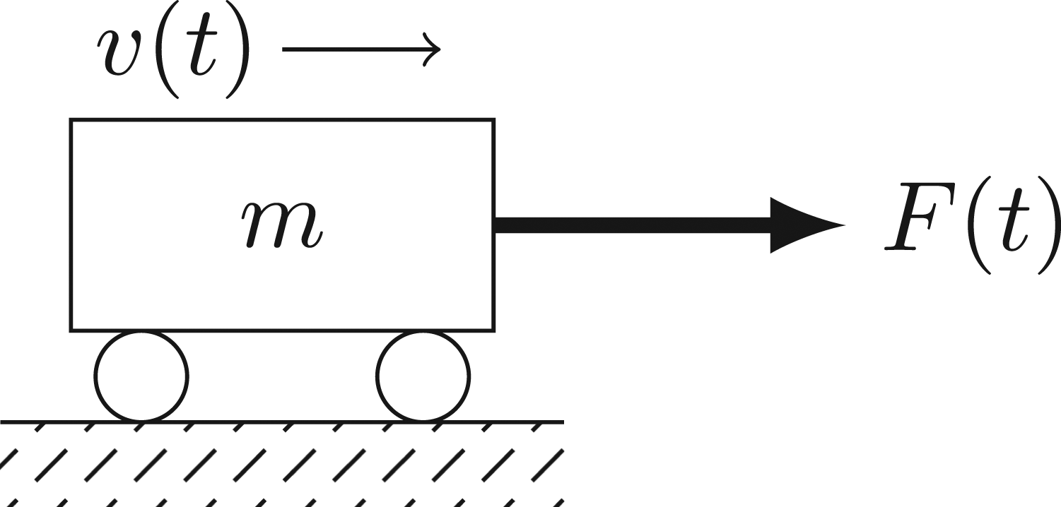

Then

T = \frac{k}{m (τ s + 1)}

(18)

Suppose that k = m. Then at s = 0, T = 1, so the interpolation condition is met.¹⁴ We will find the corresponding controller

S = 1 - T = \frac{τ s}{τ s + 1} where S = (1 - G_{p} Y)

(19)

G_{c} = \frac{Y}{S} = \frac{m s}{τ s + 1} \frac{τ s + 1}{τ s}

(20)

\Rightarrow G_{c} = \frac{m}{τ}

(21)

where S is the sensitivity transfer function and G_c is a pure gain, in this case proportionally equivalent to the mass m and inversely proportional to the time constant τ. The return ratio transfer function is given by

L = \frac{m}{τ} \frac{1}{m s} = \frac{1}{τ s}

(22)

For the sake of this simple example, let’s assume both m and τ are equal to one. In this case,

L = \frac{1}{s}

, G_c = 1, , and

S = \frac{s}{s + 1}

. All closed-loop transfer functions are stable, so we can proceed to looking at bandwidth.

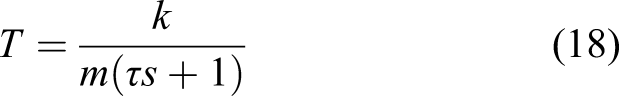
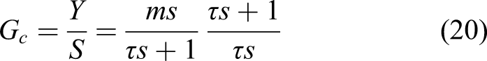
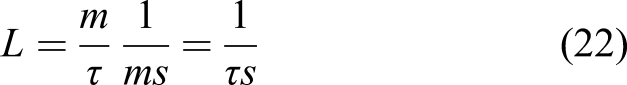
Figure 5 illustrates the closed-loop complementary sensitivity (T in solid blue), sensitivity (S in dashed red), and the return ratio (L in dot-dashed yellow) transfer functions. Note that this is a plot of the frequency response of the system, plotting the magnitude of the output when the transfer functions T, S, and Y are subject to a unit sinusoidal input u = sin ωt. The x-axis of this plot represents the input frequency ω and the y-axis is the magnitude of the output response at that frequency, measured in decibels. We identify ω_BC as the frequency where S comes within 2% of its final value. S has a final value of 1 (or 0 dB), so ω_BC will be the frequency where ω is bounded by 0.98 ≤ M_S(ω) ≤ 1.02 (or −0.175 dB ≤ M_S(ω) ≤ 0.172 dB), where M_S(ω) denotes the magnitude of S. From Figure 5, we identify that the frequency ω_BC is around 5 rad/sec.

Figure 5.

Closed-loop and return ratio transfer functions.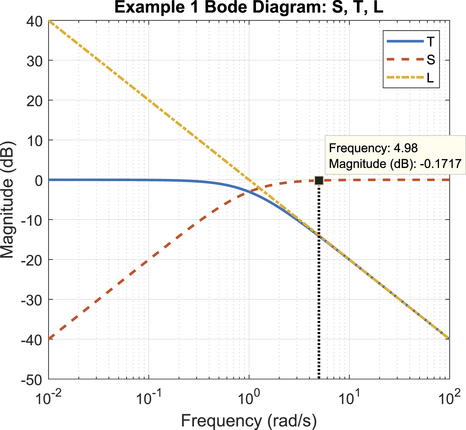

The Youla (Y in solid blue) and the controller (G_c in dashed red) transfer functions are shown in Figure 6. It is again around 5 rad/sec, where Youla reaches 2% of its final value. Given that G_c = 1, this is the frequency where the 0.98 ≤ M_Y(ω) ≤ 1.02 (or −0.175 dB ≤ M_Y(ω) ≤ 0.172 dB), where M_Y(ω) denotes the magnitude of Y.

Figure 6.

Controller and youla transfer functions.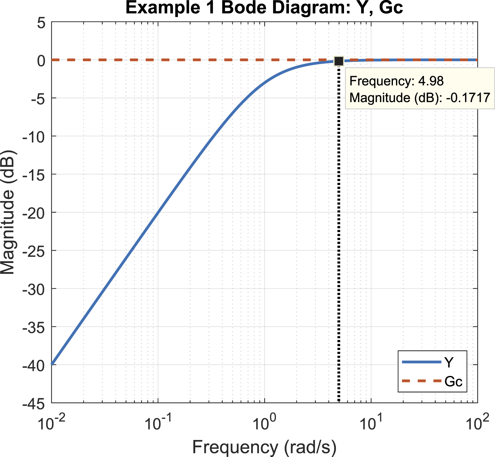

Finally, the neoclassical bandwidth measure is shown in the time domain response of S for a sinusoidal input at ω = ω_BC. That is

u (t) = \sin 4.98 t

(23)

This response is shown in Figure 7. We can see that as e(t) approaches the steady-state response, the it is bounded within ±2% of 1 = 0 dB, the final magnitude of S as ω → ∞.

Figure 7.

Error response in the time domain for a sinusoidal input at the neoclassical bandwidth frequency.

Figures 5 to 7 all show the usefulness of the controller G_c has decayed with increasing frequency. For this example, the neoclassical bandwidth was measured for a selected α = 0.02, meaning it indicates the frequency at which 2% of information from the output is fed back. The control designer would then Note that other values of α, such as α = 0.5, α = 0.1, etc.…could have been chosen.

Example 2 Consider again a force F(t) applied to a mass again, but this time, to control position rather than velocity. This system is shown in Figure 8.

\frac{\hat{y}}{\hat{u}} = \frac{1}{m s^{2}}

(24)

We choose a Youla parameter to cancel the dynamics of the mass.

Y = \frac{m k s^{2}}{{(τ s + 1)}^{2}}

(25)

Figure 8.

Single mass system with force input and position output.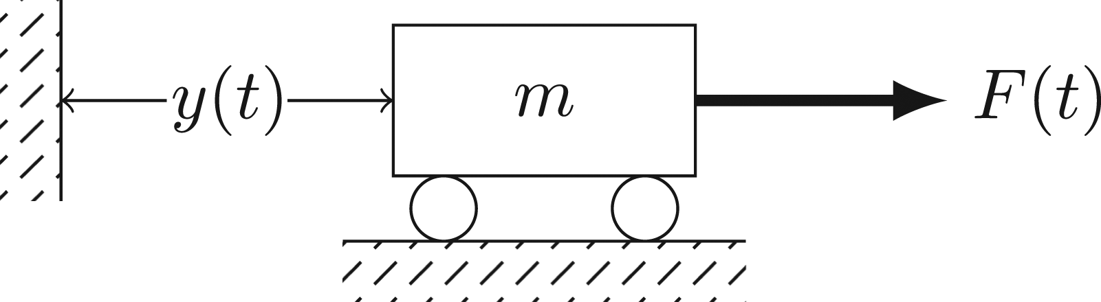

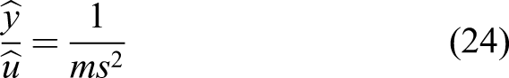
Then

T = \frac{k}{{(τ s + 1)}^{2}}

(26)

The interpolation conditions to ensure internal stability are T (0) = 1 and

\frac{d T (0)}{d s} = 0

T (0) = \frac{k}{{(τ \cdot 0 + 1)}^{2}} = 1

(27)

Therefore k = 1. So

{\frac{d T}{d s} |}_{s = 0} = \frac{- 2 τ}{{(τ \cdot 0 + 1)}^{3}} = 0

(28)

Therefore, τ = 0. This means we now have

Y = m s^{2}

(29)

Y is now improper, which is unacceptable.

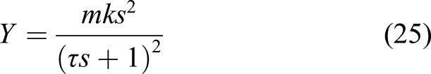
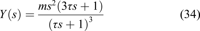
If we add a zero to the proposed Youla transfer function, it can be shown the interpolation conditions could be met.⁸ Therefore, we next consider

Y (s) = \frac{m s^{2} (τ_{1} s + 1)}{{(τ s + 1)}^{3}}

(30)

That is, an additional pole and zero are added to Y with an extra tuning parameter τ₁. Thus

T (s) = \frac{(τ_{1} s + 1)}{{(τ s + 1)}^{3}}

(31)

The first interpolation condition, T (0) = 1, is satisfied and it is straightforward to show that

\frac{d T (0)}{d s}

can be written as

\frac{d T (0)}{d s} = {[\frac{τ_{1}}{{(τ s + 1)}^{3}} - \frac{3 τ (τ_{1} s + 1)}{{(τ s + 1)}^{4}}] |}_{s = 0}

(32)

= τ_{1} - 3 τ = 0

(33)

so that an internally stabilizing value of the Youla transfer function is

Y (s) = \frac{m s^{2} (3 τ s + 1)}{{(τ s + 1)}^{3}}

(34)

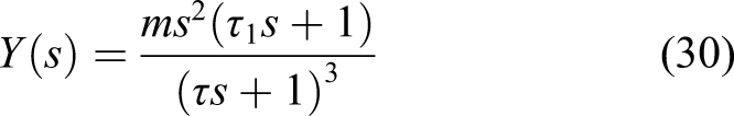
An internally-stabilizing compensator is calculated similar to the previous example.

G_{c} (s) = \frac{m s^{2} \frac{(3 τ s + 1)}{{(τ s + 1)}^{3}}}{1 - \frac{(3 τ s + 1)}{{(τ s + 1)}^{3}}}

(35)

= \frac{m s^{2} (3 τ s + 1)}{τ^{2} s^{2} (τ s + 3)}

(36)

= \frac{m}{3 τ^{2}} \frac{(3 τ s + 1)}{(\frac{τ}{3}) s + 1}

(37)

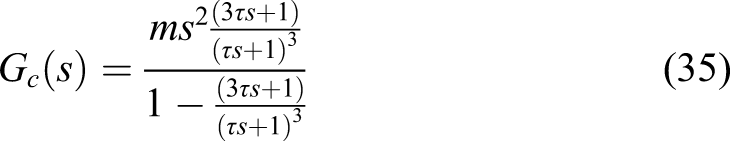
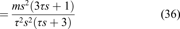
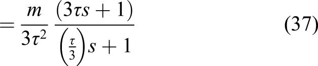
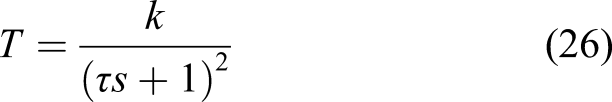
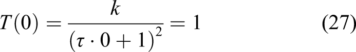
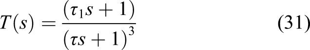
This turns out to be a lead controller. As a check for internal stability, we consider the fact that G_cG_p does not contain the wrong kind of cancellation (cancellation in the RHP or on jω-axis). Also, T(s) = (3τs + 1)/(τs + 1)³ so that the closed-loop is stable; as a matter of fact, we have placed all three closed-loop poles at s = − 1/τ in this example. It should be noted that by using this approach, we have the flexibility to select Youla and shape the closed-loop transfer function T any way we desire, but we have to meet interpolation conditions in order to result in internal stability. So long as Y is selected per equation (34), all closed-loop transfer functions will be stable, so we can proceed to looking at bandwidth.

Figure 9 illustrates the closed-loop transfer functions T and S (in blue and dashed red) and the return ratio L (in dot-dashed yellow). Again, the frequency ω_BC is marked on this figure, where according to the aforementioned theorem, it is the frequency where |T| → |L|, |S| → 1, and Y → |G_c|.

Figure 9.

Closed-loop and return ratio transfer functions.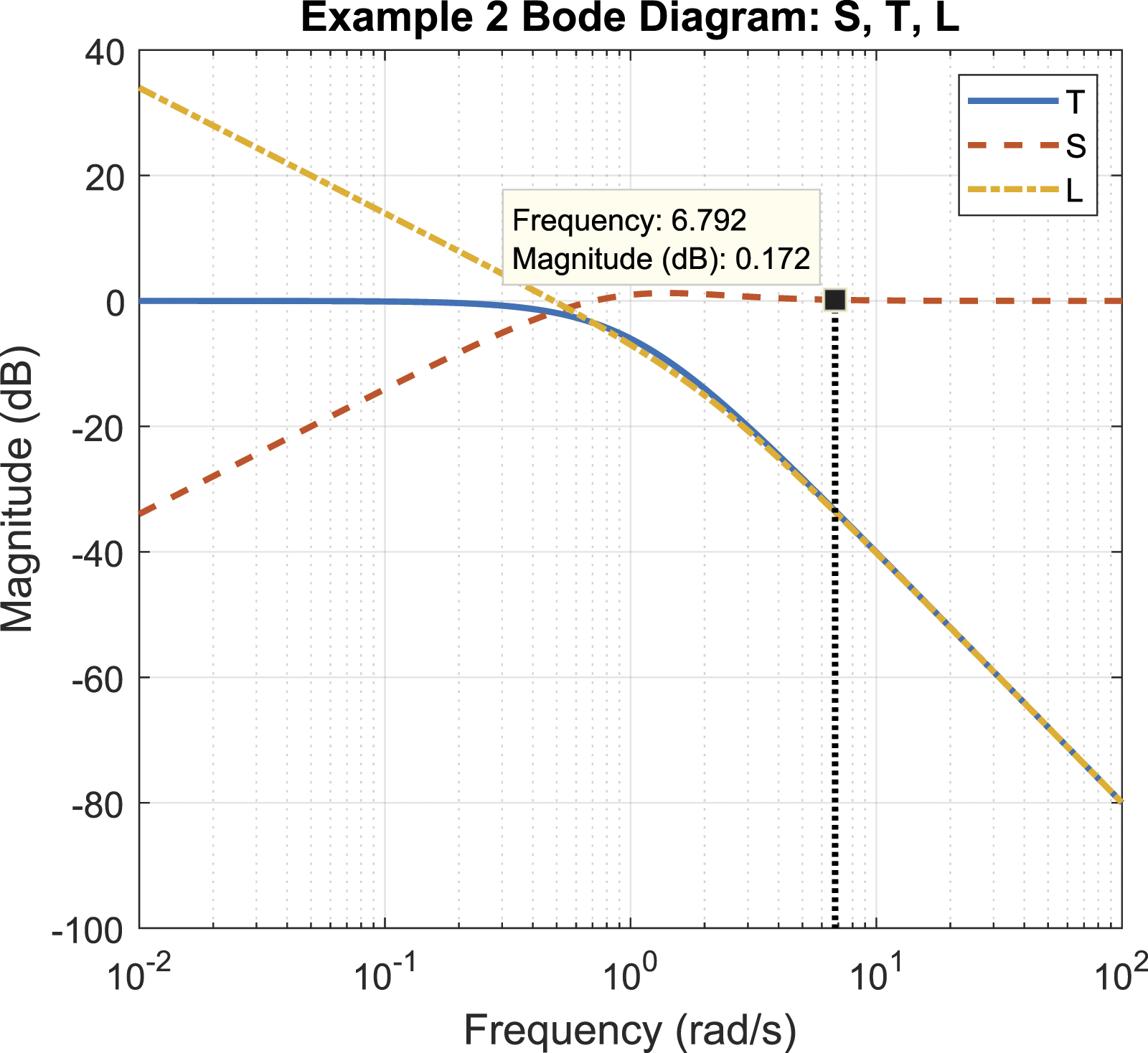

As in the last example, we identify ω_BC as the frequency where S comes within 2% of its final value. S has a final value of 1 (or 0 dB), so ω_BC will be the frequency where ω is bounded by 0.98 ≤ M_S(ω) ≤ 1.02 (or −0.175 dB ≤ M_S(ω) ≤ 0.172 dB). From Figure 9, we identify that the frequency ω_BC is around 6.8 rad/sec.

The frequency where Y → |G_c| is illustrated in Figure 10. This frequency corresponds to the same frequency ω_BC in Figure 9.

Figure 10.

Controller and youla transfer functions.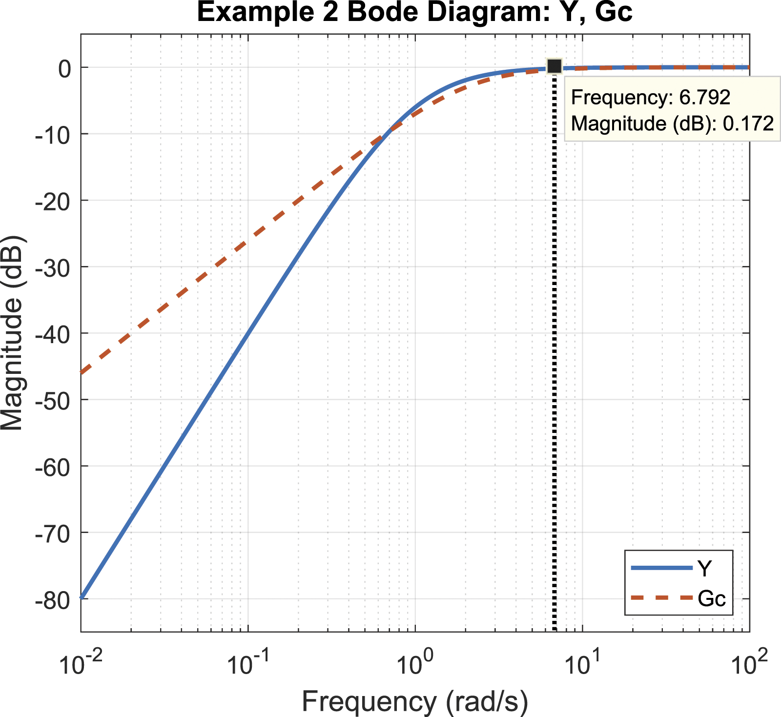

Finally, the neoclassical bandwidth measure is shown in the time domain response of S for a sinusoidal input at ω = ω_BC. That is

u (t) = \sin 6.972 t

(38)

This response is shown in Figure 11. We can see that as e(t) approaches the steady-state response, it is bounded within ±2% of 1 = 0 dB, the final magnitude of S as ω → ∞.

Figure 11.

Error response in the time domain for a sinusoidal input at the neoclassical bandwidth frequency.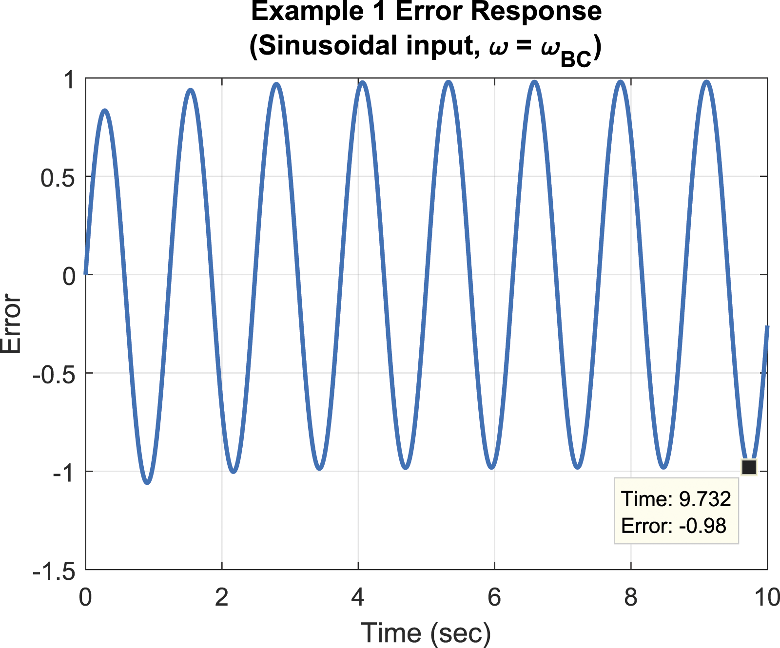

As in the first example, Figures 9 to 11 all show the usefulness of the controller G_c has decayed with increasing frequency, and in particular at ω = ω_BC, it has decayed to the point where only 2% of information from the output is fed back. Interestingly, we see that ω_BC corresponds to a positive decibel value of S, unlike in the first example. However, this still corresponds to the same decay in usefulness of the controller G_c.

Conclusions

The concept of closed-loop control system bandwidth has been discussed in many control texts and publications in the past. This concept is not well defined when one tries to use this frequency to relate the speed of closed-loop response in time domain due to inputs such as the unit step to a corresponding frequency known as closed-loop bandwidth in the frequency domain. It turns out that when one tries to extend the concept of bandwidth to the frequency at which benefits of feedback is lost, then the definitions of closed-loop bandwidth simply do not play a role. In this work, we proposed a new and precise measure which is directly related to a particular frequency of the closed-loop feedback systems after which the benefits of feedback control are lost. We showed that high frequency asymptotes of three closed-loop transfer functions, T, S and Y are exactly the same asymptotes as when feedback information is lost. We modeled this information through a binary number α.

Future work will entail extending this measure of bandwidth from the simple examples given in this paper to more complex controller design problems. By using the refined understanding of the frequencies over which a controller is useful, a more robust and effective controller could be designed. Applications of this include, for example, topics in vehicle dynamics and control,¹⁵ state estimation,^16,17 or systems with substantial time delay.^18,19

Footnotes

Acknowledgments

We would like to thank University of California, Davis for their generous support of this work.

Declaration of conflicting interests

The author(s) declared no potential conflicts of interest with respect to the research, authorship, and/or publication of this article.

Funding

The author(s) received no financial support for the research, authorship, and/or publication of this article.

ORCID iD

Francis Assadian

References

Skogestad

Postlethwaite

. Multivariable feedback control: analysis and design, volume 2. Citeseer, 2007.

Brewer

. MAE 272 - Real and Complex Analysis in Signal, Dynamic System, and Feedback Theories. Lecture Notes, University of California, Davis, 1995.

Franklin

Powell

Workman

et al. Digital control of dynamic systems, volume 3. Addison-Wesley Reading, MA, 1998.

Franklin

Powell

Emami-Naeini

et al. Feedback control of dynamic systems, volume 4. Prentice-Hall Upper Saddle River, NJ, 2002.

Morari

Zafiriou

. Robust process control. Morari, 1989.

Nise

. Control systems engineering. 7th ed. John Wiley & Sons, 2015.

Youla

Bongiorno

. Single-loop feedback-stabilization of linear multivariable dynamical plants. Automatica 1974; 10(2): 159–173. DOI:10.1016/0005-1098(74)90021-1.

Assadian

MAE 273A - SISO optimal robust control. Lecture Notes, University of California, Davis, 2018.

Vidyasagar

. Control system synthesis: a factorization approach, part II. Morgan and Claypool Publishers, 2011.

10.

Velazquez Alcantar

Assadian

Kuang

et al. Optimal longitudinal slip ratio allocation and control of a hybrid electric vehicle with eawd capabilities. In: ASME 2016 Dynamic Systems and Control Conference. American Society of Mechanical Engineers Digital Collection.

11.

Zhou

. A natural approach to high performance robust control: another look at youla parameterization. In: SICE 2004 Annu Conf, volume 1. IEEE, pp. 869–874.

12.

Mahtout

Navas

Milanés

et al. Advances in youla-kucera parametrization: A review. Annu Rev Control 2020.

13.

Maciejowski

. Multivariable Feedback Design. 1st ed. Wokingham, UK: Addison-Wesley, 1989.

14.

Doyle

Francis

Tannenbaum

. Feedback control theory. Courier Corporation, 2013.

15.

Filipozzi

Assadian

Kuang

et al. An investigation into the traction and anti-lock braking system control design, SAE Technical Paper, 2020.

16.

Liu

Assadian

Mallon

. Vehicle yaw rate and sideslip estimations: a comparative analysis of siso and mimo youla controller output observer, linear and nonlinear kalman filters, and kinematic computation. J Mech Aerospace Eng 2019; 1(1).

17.

Filipozzi

Assadian

Kuang

, et al. Estimation of tire normal forces including suspension dynamics. Energies 2021; 14(9): 2378.

18.

Pujol-Vazquez

Mobayen

Acho

. Robust control design to the furuta system under time delay measurement feedback and exogenous-based perturbation. Mathematics 2020; 8(12): 2131.

19.

Rasoolinasab

Mobayen

Fekih

, et al. A composite feedback approach to stabilize nonholonomic systems with time varying time delays and nonlinear disturbances. ISA Transactions 2020; 101: 177–188.

A new measure to describe the feedback control systems usefulness

Abstract

Keywords

Introduction

Information as a precise measure of bandwidth

Neoclassical feedback control

Defining a measure to characterize the usefulness of feedback

Computation of new bandwidth

Proof

Examples

Conclusions

Footnotes

Acknowledgments

Declaration of conflicting interests

Funding

ORCID iD

References