Optimal design of an improved X ¯ and R control chart for joint monitoring of process location and dispersion

Abstract

Enhancing the detection power of control charts for detecting small to moderate process changes is always the focus of attention in academia. To improve the detection ability of conventional $\overline{X}$ and R control charts, an improved joint $\overline{X}$ and R chart, which combines the ordinary $\overline{X}$ and R charts with runs rules of the type ‘r out of m’, is proposed to monitor the process location and dispersion simultaneously. A finite Markov chain imbedding approach is employed to develop the resulting control scheme. A comparative study is conducted to investigate the performance of the proposed chart in terms of the out-of-control average run length. The statistical performance of the suggested chart when the process parameters are estimated is also evaluated. The numerical results indicate that (1) the proposed chart improves the detection ability of traditional $\overline{X}$ and R charts in detecting small to moderate process shifts; (2) the suggested scheme performs better than the EWMA and CUSUM schemes in detecting large process fluctuations. Furthermore, when specific values of r and m are selected, the statistical performance of the proposed chart for detecting small shifts is close to or even better than that of its competitors; (3) the run length performance of the proposed chart is greatly affected by parameter estimation, especially for small process shifts.

Introduction

Statistical process control (SPC) is a well-known technique to measure, surveil and control processes by employing statistical analysis for the sake of achieving production/service process stability and reducing process variability for improving capability. ¹ In SPC, control charts are the most popular and commonly used tool to monitor the process location or/and dispersion. In practices, among different kinds of control charts, Shewhart-type control charts are used most often owing to the characteristic of simple to understand, implement and use. Unfortunately, as pointed out by Montgomery, ¹ although Shewhart control charts are efficient to detect large process shifts, they have poor sensitivity for detecting small changes in a process.

To overcome this shortcoming, an effective approach is to design control charts with supplementary runs rules. The use of runs rules in control chart design can be traced back to the 1940s. At this period, some scholars, such as Mosteller ² and Wolfowitz, ³ tried to supplement the basic control-chart criteria with additional runs rules. Afterwards, a set of decision rules derived from runs and scans were systematically presented by Western Electric. ⁴ This work promotes worldwide the use of runs rules in the area of SPC. Koutras et al. ⁵ reviewed the literature pertinent to the Shewhart control chart with supplementary runs rules. In general, runs rules-based control charts are mainly employed to monitor the process location and/or dispersion.

The research of how to monitor the location of a production process using control charts supplied with runs rules can refer to Koutras et al. ⁵ and the literature therein. The articles debating this topic are rich in recent years. Recently, Tran ⁶ proposed a runs rules-based t chart to detect shifts in the process mean. Mehmood et al. ⁷ developed two design structures of $\overline{X}$ control chart by covering the cases of various process distributions, unknown and known parameters and runs rules. Adeoti and Malela-Majika ⁸ developed a double exponentially weighted moving average (EWMA) chart supplemented with runs rules to detect small location shifts in the process. For more examples, see Das et al., ⁹ Parkhideh and Parkhideh, ¹⁰ Lee and Khoo, ¹¹ Mehmood et al., ¹² Shongwe et al. ¹³ and so on. Comparatively speaking, little research has been carried out in the field of control charts for examining the process dispersion using the advantages provided by the employment of runs rules. Recently Antzoulakos and Rakitzis ¹⁴ introduced a runs rules-based S control chart to monitor decreases and/or increases in the process variance. Inspired by the work of Antzoulakos and Rakitzis, ¹⁴ Rakitzis and Antzoulakos ¹⁵ further considered a variable sampling interval S chart supplied with switching and signalling rules derived from runs. Some other works focused on this issue can also be seen in Nelson, ¹⁶ Lowry et al., ¹⁷ Klein, ¹⁸ Zhang and Wu. ¹⁹

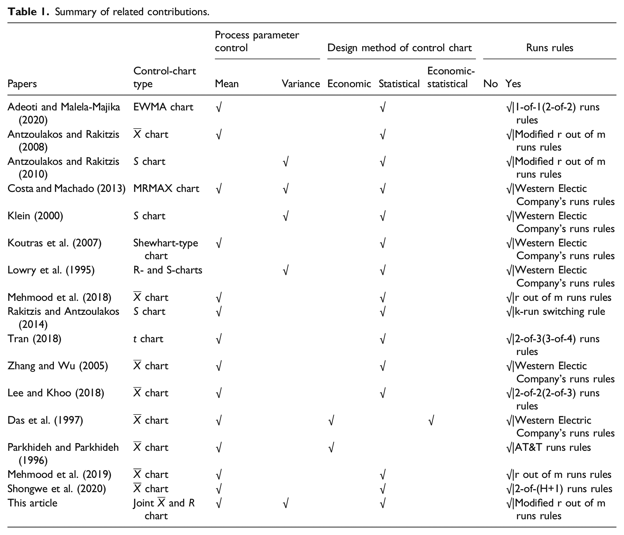
In many cases, the simultaneous monitoring of the process location and dispersion is necessary when the quality characteristic of a target process is a variable. However, all the papers mentioned above are either focused on the use of runs rules-based control chart to monitor the process mean or on the use of runs rules-based control chart to monitor the process variance. To the best of our knowledge, only one research concerning the problem of joint monitoring of process location and variability by use of control charts with supplementary runs rules is reported, see Costa and Machado. ²⁰ The authors developed a MRMAX chart to monitor the covariance matrix, and the mean vector of multivariate processes based on the sample ranges and the standardized sample means. However, the design of the MRMAX chart needs to use highly sophisticated mathematics and statistical theory. It may be too complex to use for shop floor workers. In academia and industry, the joint $\overline{X}$ and R chart is usually seen as the most commonly used control-chart tool to monitor both the process location and dispersion. As Duncan ²¹ noted, if the quality characteristic of interest is measured on a continuous scale, the simultaneous use of an $\overline{X}$ control chart to monitor the process location and an R control chart to monitor the process dispersion can provide pretty good control of the entire process. However, the joint $\overline{X}$ and R chart is insensitive to the detection of small to moderate process shifts. ²² Undoubtedly, a remedial action promoted to overcome this shortcoming is to design the joint $\overline{X}$ and R control chart with additional runs rules. Table 1 presents a summarization of the characteristics of the existing related researches.

Table 1.

Summary of related contributions.

Papers	Control-chart type	Process parameter control		Design method of control chart			Runs rules
		Mean	Variance	Economic	Statistical	Economic-statistical	No	Yes
Adeoti and Malela-Majika (2020)	EWMA chart	√			√			√|1-of-1(2-of-2) runs rules
Antzoulakos and Rakitzis (2008)	$\overline{X}$ chart	√			√			√|Modified r out of m runs rules
Antzoulakos and Rakitzis (2010)	S chart		√		√			√|Modified r out of m runs rules
Costa and Machado (2013)	MRMAX chart	√	√		√			√|Western Electic Company’s runs rules
Klein (2000)	S chart		√		√			√|Western Electic Company’s runs rules
Koutras et al. (2007)	Shewhart-type chart	√			√			√|Western Electic Company’s runs rules
Lowry et al. (1995)	R- and S-charts		√		√			√|Western Electic Company’s runs rules
Mehmood et al. (2018)	$\overline{X}$ chart	√			√			√|r out of m runs rules
Rakitzis and Antzoulakos (2014)	S chart	√			√			√|k-run switching rule
Tran (2018)	t chart	√			√			√|2-of-3(3-of-4) runs rules
Zhang and Wu (2005)	$\overline{X}$ chart	√			√			√|Western Electic Company’s runs rules
Lee and Khoo (2018)	$\overline{X}$ chart	√			√			√|2-of-2(2-of-3) runs rules
Das et al. (1997)	$\overline{X}$ chart	√		√		√		√|Western Electric Company’s runs rules
Parkhideh and Parkhideh (1996)	$\overline{X}$ chart	√		√				√|AT&T runs rules
Mehmood et al. (2019)	$\overline{X}$ chart	√			√			√|r out of m runs rules
Shongwe et al. (2020)	$\overline{X}$ chart	√			√			√|2-of-(H+1) runs rules
This article	Joint $\overline{X}$ and R chart	√	√		√			√|Modified r out of m runs rules

In the present article, a joint $\overline{X}$ and R control chart supplemented with runs rules of the type ‘r out of m’ for the detection of small and moderate changes in process location and dispersion is introduced. A finite Markov chain imbedding approach is employed to describe and evaluate the average run length of the proposed chart. A comparison study is carried out to highlight the superior statistical performance of the proposed chart in terms of the out-of-control average run length.

The remainder of this article is organized as follows. An introduction of the conventional joint $\overline{X}$ and R chart is presented in Section 2. Section 3 provides the concept of the proposed control-chart scheme. Section 4 gives the computation process of ARL for the proposed chart. The statistical design model of the proposed chart is developed in Section 5. Section 6 presents a comparative study to justify the effectiveness of the suggested model. The effects of parameter estimation on the proposed chart are also studied. Finally, Section 7 summarizes the conclusions of the study.

The joint $\overline{X}$ and R control chart

Assume that a production process subject to a single assignable cause is monitored by a joint $\overline{X}$ and R control chart. The production process is assumed to be in a state of statistical control with variance ${\sigma }^2={\sigma }_0^2$ and mean μ = μ ₀ at the start of the process, where σ ₀ and μ ₀ represent the target standard deviation value and the target mean value, respectively. It is also assumed that the measurable quality characteristic of interest X of the process is a normally distributed random variable. At some random time in the future, the occurrence of the assignable cause may shift the process location from μ ₀ to μ ₁ = μ ₀ ± δσ ₀(δ > 0) and/or increase the process standard deviation from σ ₀ to σ ₁ = γσ ₀(γ > 1). Without loss of generality, we assume the time length required for the occurrence of the assignable cause is an exponential distributed random variable.

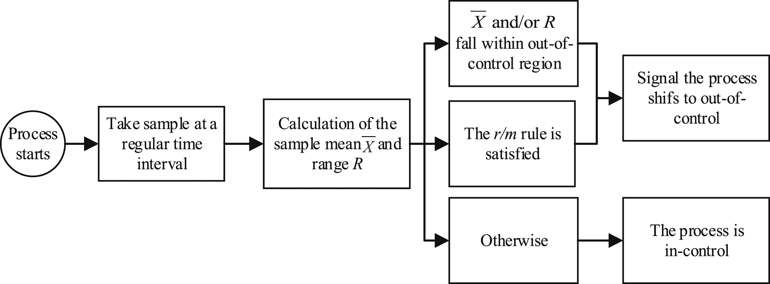
Random samples of size n(n ∈ N ⁺) are taken from the production process at regular time intervals. Once a sample is taken, two statistics, the mean $\overline{X}$ and the range R of the sample, are computed and plotted on the $\overline{X}$ and R sub-charts, respectively. When the mean point is beyond (below) the upper (lower) control limit of the $\overline{X}$ sub-chart and/or when the range point is beyond (below) the upper (lower) control limit of the R sub-chart, the process is deemed to be out of control. An investigation for the assignable cause will then be undertaken. Otherwise, the process is deemed to be in control.

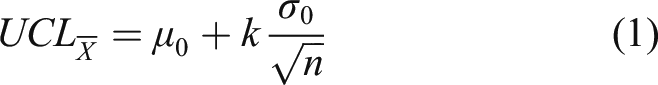
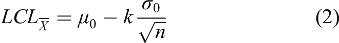
The five parameters, including the sampling interval h, the sample size n and the control limit coefficient k(≥ 0) of the $\overline{X}$ sub-chart, and the upper and lower control limit coefficients, U _R and L _R , of the R sub-chart, are necessary to be predetermined to design an ordinary $\overline{X}$ and R chart. The upper and lower control limits, $UC{L}_{\overline{X}}$ and $LC{L}_{\overline{X}}$ , of the $\overline{X}$ sub-chart can be, respectively, given as follows

$$UC{L}_{\overline{X}}={\mu }_0+k\frac{{\sigma }_0}{\sqrt{n}}$$

(1)

$$LC{L}_{\overline{X}}={\mu }_0-k\frac{{\sigma }_0}{\sqrt{n}}$$

(2)

Denote s ₍₁₎, s ₍₂₎, …, s _(n) as a sample randomly sampled from the normally distributed process having mean μ ₀ and standard deviation σ ₀. Further assume that these observations are already arranged in ascending order of magnitude. Denote by R = s _(n) − s ₍₁₎ the range of the sample. Then, the upper and lower control limits, UCL _R and LCL _R , of the R sub-chart can be, respectively, calculated as

$$UC{L}_R={\sigma }_0{U}_R$$

(3)

$$LC{L}_R={\sigma }_0{L}_R$$

(4)

The average run length (ARL), which represents the average number of observations or samples required to send a control-chart signal, is usually seen as the most popular performance criteria to evaluate the performance of the control chart considered. The ARL of an ordinary $\overline{X}$ and R chart can be calculated as following.

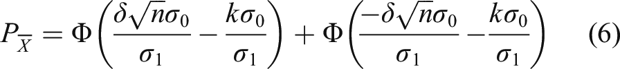
Let ${\alpha }_{\overline{X}}$ and $P_{\overline{X}}$ be the Type-I error (i.e. the occurrence of a false alarm) rate and the detection ability (i.e. the probability of sending a true alarm) of the $\overline{X}$ sub-chart, respectively. ${\alpha }_{\overline{X}}$ and $P_{\overline{X}}$ can be, respectively, given by

$${\alpha }_{\overline{X}}=2\left[1-\mathrm{\Phi }\left(k\right)\right]$$

(5)

and

$$P_{\overline{X}}=\mathrm{\Phi }\left(\frac{\delta \sqrt{n}{\sigma }_0}{{\sigma }_1}-\frac{k{\sigma }_0}{{\sigma }_1}\right)+\mathrm{\Phi }\left(\frac{-\delta \sqrt{n}{\sigma }_0}{{\sigma }_1}-\frac{k{\sigma }_0}{{\sigma }_1}\right)$$

(6)

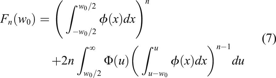
For R sub-chart, let W ₀ be the standardized range, it then has $W_0=R/{\sigma }_0$ . The cumulative distribution function for random variable W ₀ can be found, which can be given as (refer to Rahim ²³ )

$$\begin{array}{l}{F}_n\left(w_0\right)={\left({\displaystyle {\int }_{-w_0/2}^{w_0/2}\varphi \left(x\right)dx}\right)}^n\\ +2n{\displaystyle {\int }_{w_0/2}^{\infty }\mathrm{\Phi }\left(u\right)}{\left({\displaystyle {\int }_{u-w_0}^u\varphi \left(x\right)dx}\right)}^{n-1}du\end{array}$$

(7)

where

$$\varphi \left(x\right)={\left(2\pi \right)}^{-1/2}{e}^{-x^2/2}$$

(8)

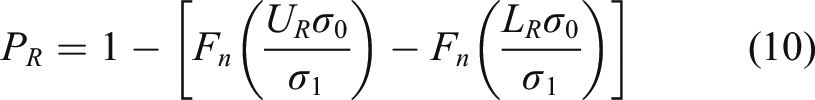
Let α _R and P _R be the Type-I error rate and the detection power of the R sub-chart, respectively. Then, α _R and P _R can be separately given by

$${\alpha }_R=1-\left[F_n\left(U_R\right)-F_n\left(L_R\right)\right]$$

(9)

$$P_R=1-\left[F_n\left(\frac{U_R{\sigma }_0}{{\sigma }_1}\right)-F_n\left(\frac{L_R{\sigma }_0}{{\sigma }_1}\right)\right]$$

(10)

Thus, the false alarm probability α _j of the joint $\overline{X}$ and R chart can be calculated as

$${\alpha }_j={\alpha }_{\overline{X}}+{\alpha }_R-{\alpha }_{\overline{X}}\times {\alpha }_R$$

(11)

The detection capacity P _j of the joint $\overline{X}$ and R chart is

$$P_j=P_{\overline{X}}+P_R-P_{\overline{X}}\times P_R$$

(12)

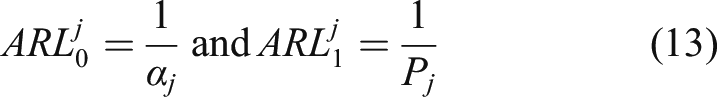
Then, the in-control ARL (denoted by $AR{L}_0^j$ ) and the out-of-control ARL (denoted by $AR{L}_1^j$ ) for the joint $\overline{X}$ and R chart can be, respectively, given as

$$AR{L}_0^j=\frac{1}{{\alpha }_j}\hspace{0.17em}\hspace{0.17em}\mathrm{and}\hspace{0.17em}AR{L}_1^j=\frac{1}{P_j}$$

(13)

The joint $\overline{X}$ and R chart supplemented with r out of m runs rules

The r out of m (m > r > 1 and m, r ∈ N ⁺) runs rules (denoted by r/m runs rules for convenience) proposed by Antzoulakos and Rakitzis ²⁴ has been proven to enhance the sensitivity of control charts for detecting small process mean shifts. The basic design concept of a control chart supplemented with r/m runs rules is given as follows: the chart will signal an out-of-control situation when either r points plot outside of an UCL which are parted by at most (m − r) sample points between the UCL and the central line of the chart or r points plot outside of a LCL which are parted by at most (m − r) sample points between the LCL and the central line of the chart. In the following context, the joint $\overline{X}$ and R chart supplemented with r/m runs rules is called $\overline{X}|R:r/m$ chart for short. Similar to the implementation of the conventional $\overline{X}$ and R chart, the $\overline{X}:r/m$ and R: r/m sub-charts will be introduced, respectively.

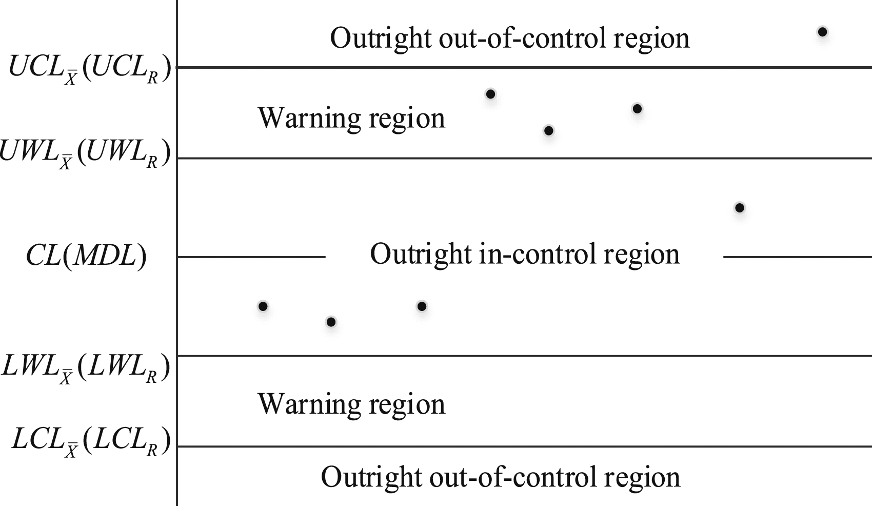
For implementing the $\overline{X}:r/m$ sub-chart, five control limits including the lower and the upper control limits ( $LC{L}_{\overline{X}}$ and $UC{L}_{\overline{X}}$ ), the central line ( $C{L}_{\overline{X}}$ ), and two warning control limits ( $LW{L}_{\overline{X}}$ and $UW{L}_{\overline{X}}$ ) should be pre-established. The design of control charts supplied with warning limits was first studied by Page, ²⁵ and this design concept has then been widely promoted in the field of SPC. The five lines satisfy the inequality $LC{L}_{\overline{X}}<LW{L}_{\overline{X}}<C{L}_{\overline{X}}<UW{L}_{\overline{X}}<UC{L}_{\overline{X}}$ . These control limits can then be calculated as follows

$$UC{L}_{\overline{X}}={\mu }_0+k_1\frac{{\sigma }_0}{\sqrt{n}}, UW{L}_{\overline{X}}={\mu }_0+k_2\frac{{\sigma }_0}{\sqrt{n}}$$

(14)

$$C{L}_{\overline{X}}={\mu }_0$$

(15)

$$LW{L}_{\overline{X}}={\mu }_0-k_2\frac{{\sigma }_0}{\sqrt{n}}, LC{L}_{\overline{X}}={\mu }_0-k_1\frac{{\sigma }_0}{\sqrt{n}}$$

(16)

where k ₁ and k ₂ (k ₁ ≥ k ₂) are the control limit coefficients.

Similarly, in order to implement the R: r/m sub-chart, five control limits containing the lower and the upper control limits (LCL _R and UCL _R ), the median limit (ML), and two warning control limits (LWL _R and UWL _R ) should be predetermined. The five control limits satisfy LCL _R < LWL _R < ML < UWL _R < UCL _R . It is worth noting the ML is used here to replace the central line of the chart. Montgomery ¹ and Nelson ¹⁶ declared that the ML can be used as the central line of S and R control charts so that the number of runs below and above the ML may remain unaffected by their asymmetrical distribution. The control limits of R: r/m sub-chart can be established as follows

$$UC{L}_R={\sigma }_0{U}_R \mathrm{and} F_n\left(w>U_R\right)={\alpha }_R/2$$

(17)

$$UW{L}_R={\sigma }_{0}U{W}_R$$

(18)

$$ML={\sigma }_0{M}_R \mathrm{and} F_n\left(w>M_R\right)=0.5$$

(19)

$$LW{L}_R={\sigma }_{0}L{W}_R$$

(20)

$$LC{L}_R={\sigma }_0{L}_R \mathrm{and} F_n\left(w>L_R\right)=1-{\alpha }_R/2$$

(21)

where U _R , UW _R , M _R , LW _R and L _R are the control limit coefficients and α _R is the false alarm rate. For both $\overline{X}:r/m$ and R: r/m sub-charts, the control limits divide the chart into three regions, namely, outright out-of-control region, warning region, and outright in-control region as shown in Figure 1.

Figure 1.

Pattern of points dropping in different regions of the $\overline{X}:r/m$ (R : r/m) sub-chart.

The operation of the joint $\overline{X}|R:r/m$ chart can then be outlined below:

Determine the five control limits (including $\mathrm{L}\mathrm{C}{\mathrm{L}}_{\overline{X}}$ ,  $\mathrm{L}\mathrm{W}{\mathrm{L}}_{\overline{X}}$ ,  $\mathrm{C}{\mathrm{L}}_{\overline{X}}$ ,  $\mathrm{U}\mathrm{W}{\mathrm{L}}_{\overline{X}}$ and $\mathrm{U}\mathrm{C}{\mathrm{L}}_{\overline{X}}$ ) of the $\overline{X}:\mathrm{r}/\mathrm{m}$ sub-chart, the five control limits (including LCL _R , LWL _R , ML, UWL _R and UCL _R ) of the R: r/m sub-chart, the sample size n and the sampling interval h.

Take a sample of n observations from the process every h hour.

The two statistics, $\overline{X}$ and R of the sample, are calculated and plotted on the $\overline{X}:\mathit{r}/\mathit{m}$ and R: r/m sub-charts, respectively.

3-1. If the sample mean $\overline{X}$ (the sample range R) falls within the outright out-of-control region, a process shift will then be signalled. The control flow goes to Step 4.

3-2. When either r mean points plot outside of the $\mathrm{U}\mathrm{C}{\mathrm{L}}_{\overline{X}}$ which are parted by at most (m − r) mean points between the $\mathrm{U}\mathrm{C}{\mathrm{L}}_{\overline{X}}$ and the $\mathrm{C}{\mathrm{L}}_{\overline{X}}$ or r points plot outside of the $\mathrm{L}\mathrm{C}{\mathrm{L}}_{\overline{X}}$ which are parted by at most (m − r) mean points between the LCL and the $\mathrm{C}{\mathrm{L}}_{\overline{X}}$ , the process is taken as out of control. The $\overline{X}|\mathit{R}:\mathit{r}/\mathit{m}$ chart produces an out-of-control signal and the control flow goes to Step 4.

3-3. When either r range points plot outside of the $\mathrm{U}\mathrm{C}{\mathrm{L}}_{\overline{X}}$ which are parted by at most (m − r) range points between the $\mathrm{U}\mathrm{C}{\mathrm{L}}_{\overline{X}}$ and the $\mathrm{C}{\mathrm{L}}_{\overline{X}}$ or r points plot outside of the $\mathrm{L}\mathrm{C}{\mathrm{L}}_{\overline{X}}$ which are parted by at most (m − r) range points between the LCL and the $\mathrm{C}{\mathrm{L}}_{\overline{X}}$ , the process is also considered as out of control. The $\overline{X}|\mathit{R}:\mathit{r}/\mathit{m}$ chart triggers an out-of-control signal and the control flow goes to Step 4.

3-4. Otherwise, the process is said to be under control. The control flow goes to Step 2.

The process stops and an investigation will be taken to locate and eliminate the assignable cause. Once the production process is brought back into an in-control condition the control flow goes back to Step 2.

Figure 2 shows the control procedure of the proposed chart. It is worth noting that if we are only concern with the detection of small process location and dispersion shifts, the $\overline{X}|R:r/m$ chart can be used without Step (3-1). However, during the operation of a process, the unusually extreme observations may be produced. If such a case occurs, the chart sending an immediate out-of-control signal will make the implement of control chart be more realistic.

Figure 2.

The control flow of the suggested chart.

Performance measure

The average run length (ARL) is the most commonly used indicator to measure the statistical performance of control charts for monitoring a process. When a process change happens, a low ARL is desirable so that the process shift can be detected timely; when the process is in an in-control state, a large ARL is desirable so that the false alarm rate of the chart considered is low. In this section, the calculation of ARL for the proposed chart is analysed.

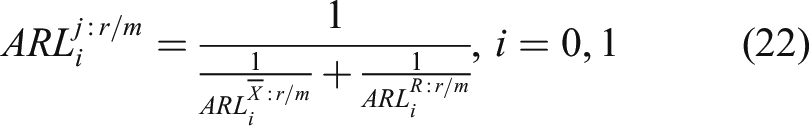
Since the implement of the $\overline{X}$ sub-chart and the R sub-chart is independent, the ARL for the joint $\overline{X}|R:r/m$ chart can be calculated by make use of the classical formula

$$AR{L}_i^{j:r/m}=\frac{1}{\frac{1}{AR{L}_i^{\overline{X}:r/m}}+\frac{1}{AR{L}_i^{R:r/m}}}, i=0,\hspace{0.17em}1$$

(22)

where $AR{L}_i^{\overline{X}:r/m}$ and $AR{L}_i^{R:r/m}$ represent the ARL of the $\overline{X}:r/m$ and R: r/m sub-charts, respectively. When i = 0, the in-control ARL is obtained; when i = 1, the out-of-control ARL is achieved. Therefore, for calculating the ARL of the joint $\overline{X}|R:r/m$ chart, the ARLs of the $\overline{X}:r/m$ and R: r/m sub-charts should be pre-calculated.

The calculation of ARL for the $\overline{X}:r/m$ sub-chart is show in the following subsection, while the ARL for the R: r/m sub-chart is shown in Appendix.

Calculation of ARL for the $\overline{X}:r/m$ sub-chart

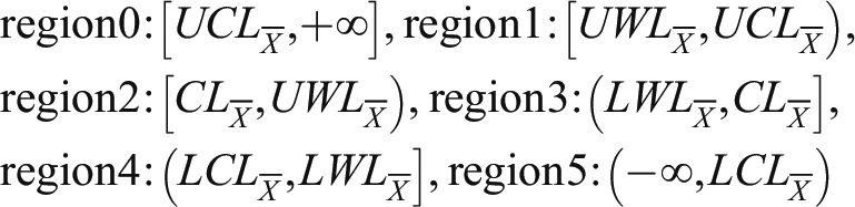
According to the description in Section 3, the five control limits of the $\overline{X}:r/m$ sub-chart divide the chart into six regions, namely

$$\begin{array}{l}\mathrm{region}\hspace{0.17em}0:\hspace{0.17em}\hspace{0.17em}\left[UC{L}_{\overline{X}},+\infty \right], \mathrm{region}\hspace{0.17em}1: \left[UW{L}_{\overline{X}},\hspace{0.17em}\hspace{0.17em}UC{L}_{\overline{X}}\right),\\ \mathrm{region}\hspace{0.17em}2:\hspace{0.17em}\hspace{0.17em} \left[C{L}_{\overline{X}},\hspace{0.17em}\hspace{0.17em}UW{L}_{\overline{X}}\right), \mathrm{region}\hspace{0.17em}3: \left(LW{L}_{\overline{X}},\hspace{0.17em}\hspace{0.17em}C{L}_{\overline{X}}\right],\\ \mathrm{region}\hspace{0.17em}4: \hspace{0.17em}\hspace{0.17em}\left(LC{L}_{\overline{X}},\hspace{0.17em}\hspace{0.17em}LW{L}_{\overline{X}}\right], \mathrm{region}\hspace{0.17em}5: \left(-\infty ,\hspace{0.17em}\hspace{0.17em}\hspace{0.17em}\hspace{0.17em}LC{L}_{\overline{X}}\right)\end{array}$$

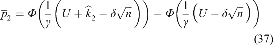
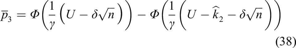
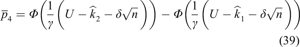
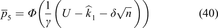
Let p ₀, p ₁, p ₂, p ₃, p ₄ and p ₅ be the probability that a mean point falls in regions 0, 1, 2, 3, 4 and 5, respectively. Then, we have

$$p_0=1-\mathrm{\Phi }\left(\frac{k_1{\sigma }_0}{{\sigma }_1}-\frac{\delta {\sigma }_0\sqrt{n}}{{\sigma }_1}\right)$$

(23)

$$p_1=\mathrm{\Phi }\left(\frac{k_1{\sigma }_0}{{\sigma }_1}-\frac{\delta {\sigma }_0\sqrt{n}}{{\sigma }_1}\right)-\mathrm{\Phi }\left(\frac{k_2{\sigma }_0}{{\sigma }_1}-\frac{\delta {\sigma }_0\sqrt{n}}{{\sigma }_1}\right)$$

(24)

$$p_2=\mathrm{\Phi }\left(\frac{k_2{\sigma }_0}{{\sigma }_1}-\frac{\delta {\sigma }_0\sqrt{n}}{{\sigma }_1}\right)-\mathrm{\Phi }\left(-\frac{\delta {\sigma }_0\sqrt{n}}{{\sigma }_1}\right)$$

(25)

$$p_3=\mathrm{\Phi }\left(-\frac{\delta {\sigma }_0\sqrt{n}}{{\sigma }_1}\right)-\mathrm{\Phi }\left(-\frac{k_2{\sigma }_0}{{\sigma }_1}-\frac{\delta {\sigma }_0\sqrt{n}}{{\sigma }_1}\right)$$

(26)

$$p_4=\mathrm{\Phi }\left(-\frac{k_2{\sigma }_0}{{\sigma }_1}-\frac{\delta {\sigma }_0\sqrt{n}}{{\sigma }_1}\right)-\mathrm{\Phi }\left(-\frac{k_1{\sigma }_0}{{\sigma }_1}-\frac{\delta {\sigma }_0\sqrt{n}}{{\sigma }_1}\right)$$

(27)

$$p_5=\mathrm{\Phi }\left(-\frac{k_1{\sigma }_0}{{\sigma }_1}-\frac{\delta {\sigma }_0\sqrt{n}}{{\sigma }_1}\right)$$

(28)

Because of difficulties in deriving the general formulate of ARL for the study of the $\overline{X}:r/m$ chart, without loss of generality, the $\overline{X}:2/4$ chart will be studied in detail as a typical instance of the whole class of $\overline{X}:r/m$ chart. The method of finite Markov chain imbedding suggested by Fu and Koutras ²⁶ is utilized for the study of the calculation of ARL for the chart considered.

Denote {X _t , t ≥ 0} be a sequence of independent and identically distributed trials taking values in the set Re = {0, 1, 2, 3, 4, 5}. Then, it has p(x _t = 0) = p ₀, p(x _t = 1) = p ₁, p(x _t = 2) = p ₂, p(x _t = 3) = p ₃, p(x _t = 4) = p ₄ and p(x _t = 5) = p ₅. Consider the compound pattern

$$\tau =\left\{\mathrm{0,11,121,1221,44,434,4334,5}\right\}$$

and let T be the length of time of the first occurrence of τ. It is then clear that the run length distribution of the $\overline{X}:2/4$ chart is coincident with the waiting time distribution T of τ. The following eight blocks can be achieved by decomposing the pattern τ

$$“1”=\left\{2,\hspace{0.17em}3\right\},“2”=1,“3”=12,“4”=122,“5”=4,$$

$$“6”=43,“7”=433$$

$$“8”=\left\{\mathrm{0,11,121,1221,44,434,4334,5}\right\}$$

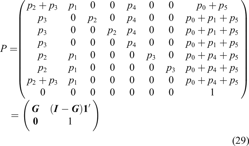
Then, the transition probability matrix of the eight blocks can be given as

$$\begin{array}{l}P=\left(\begin{array}{cccccccc}{p}_2+p_3& p_1& 0& 0& p_4& 0& 0& p_0+p_5\\ p_3& 0& p_2& 0& p_4& 0& 0& p_0+p_1+p_5\\ p_3& 0& 0& p_2& p_4& 0& 0& p_0+p_1+p_5\\ p_3& 0& 0& 0& p_4& 0& 0& p_0+p_1+p_5\\ p_2& p_1& 0& 0& 0& p_3& 0& p_0+p_4+p_5\\ p_2& p_1& 0& 0& 0& 0& p_3& p_0+p_4+p_5\\ p_2+p_3& p_1& 0& 0& 0& 0& 0& p_0+p_4+p_5\\ 0& 0& 0& 0& 0& 0& 0& 1\end{array}\right)\\ =\left(\begin{array}{cc}\mathit{G}& \left(\mathit{I}-\mathit{G}\right){\mathbf{1}}^{\prime }\\ \mathbf{0}& 1\end{array}\right)\end{array}$$

(29)

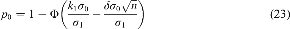
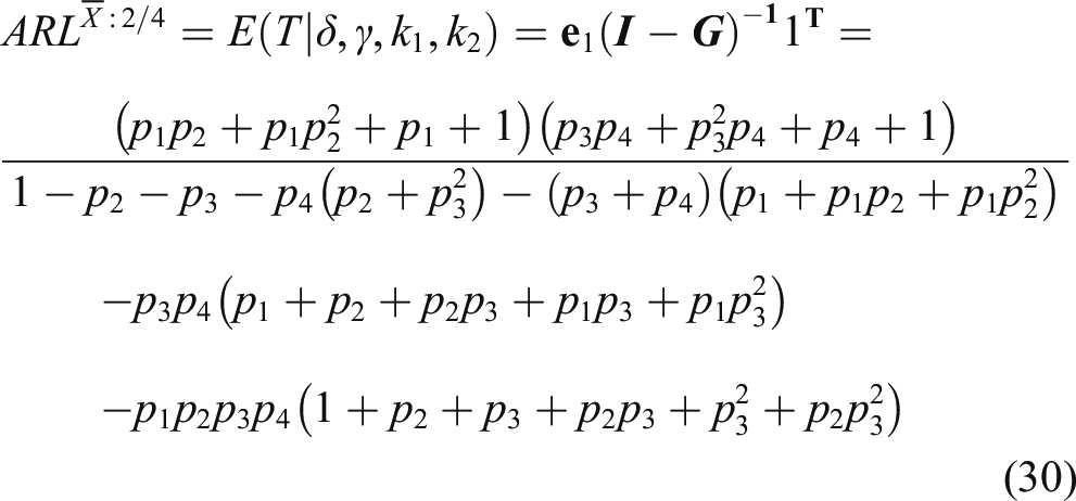
Without loss of generality, we further assume that μ ₀ = 0 and σ ₀ = 1. According to Markov’s stochastic processes theory, the ARL of the $\overline{X}:2/4$ chart can then be calculated as

$$\begin{array}{l}AR{L}^{\overline{X}:2/4}=E\left(T|\delta ,\gamma ,k_1,k_2\right)={\mathbf{e}}_1{\left(\mathit{I}-\mathit{G}\right)}^{-\mathbf{1}}{1}^{\mathbf{T}}=\\ \frac{\left(p_1{p}_2+p_1{p}_2^2+p_1+1\right)\left(p_3{p}_4+p_3^2{p}_4+p_4+1\right)}{\begin{array}{l}1-p_2-p_3-p_4\left(p_2+p_3^2\right)-\left(p_3+p_4\right)\left(p_1+p_1{p}_2+p_1{p}_2^2\right)\\ -p_3{p}_4\left(p_1+p_2+p_2{p}_3+p_1{p}_3+p_1{p}_3^2\right)\\ -p_1{p}_2{p}_3{p}_4\left(1+p_2+p_3+p_2{p}_3+p_3^2+p_2{p}_3^2\right)\end{array}}\end{array}$$

(30)

where e ₁ represents the 1th unit row vector of G , I is a (7, 7) identity matrix, and 1 is the row vector of G with all its entries being equal to 1. Then, the out-of-control ARL, $AR{L}_1^{\overline{X}:2/4}$ , of $\overline{X}:2/4$ chart can be calculated out by substituting the value of δ > 0 into equations (23-28), while the in-control ARL, $AR{L}_0^{\overline{X}:2/4}$ , can be calculated out by substituting δ = 0 into equations (23-28).

Design model

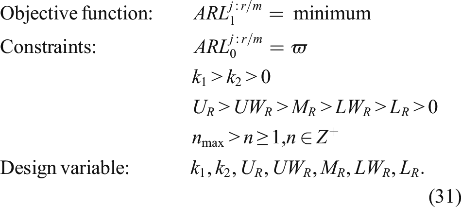
This section shows the objective function and constraints associated with the proposed model. The statistical design of a joint $\overline{X}/R:r/m$ control chart can be carried out using the optimization model as follows

$$\begin{array}{l}\mathrm{Objective}\hspace{0.17em}\mathrm{function:}\hspace{0.17em}\hspace{0.17em}\hspace{0.17em}\hspace{0.17em}\hspace{0.17em}\hspace{0.17em}\hspace{0.17em}\hspace{0.17em}\hspace{0.17em}\hspace{0.17em}\hspace{0.17em}\hspace{0.17em}AR{L}_1^{j:r/m}=\hspace{0.17em}\mathrm{minimum}\\ \mathrm{Constraints:}\hspace{0.17em}\hspace{0.17em}\hspace{0.17em}\hspace{0.17em}\hspace{0.17em}\hspace{0.17em}\hspace{0.17em}\hspace{0.17em}\hspace{0.17em}\hspace{0.17em}\hspace{0.17em}\hspace{0.17em}\hspace{0.17em}\hspace{0.17em}\hspace{0.17em}\hspace{0.17em}\hspace{0.17em}\hspace{0.17em}\hspace{0.17em}\hspace{0.17em}\hspace{0.17em}\hspace{0.17em}\hspace{0.17em}\hspace{0.17em}\hspace{0.17em}\hspace{0.17em}\hspace{0.17em}\hspace{0.17em}\hspace{0.17em}AR{L}_0^{j:r/m}=\varpi \\ \hspace{0.17em}\hspace{0.17em}\hspace{0.17em}\hspace{0.17em}\hspace{0.17em}\hspace{0.17em}\hspace{0.17em}\hspace{0.17em}\hspace{0.17em}\hspace{0.17em}\hspace{0.17em}\hspace{0.17em}\hspace{0.17em}\hspace{0.17em}\hspace{0.17em}\hspace{0.17em}\hspace{0.17em}\hspace{0.17em}\hspace{0.17em}\hspace{0.17em}\hspace{0.17em}\hspace{0.17em}\hspace{0.17em}\hspace{0.17em}\hspace{0.17em}\hspace{0.17em}\hspace{0.17em}\hspace{0.17em}\hspace{0.17em}\hspace{0.17em}\hspace{0.17em}\hspace{0.17em}\hspace{0.17em}\hspace{0.17em}\hspace{0.17em}\hspace{0.17em}\hspace{0.17em}\hspace{0.17em}\hspace{0.17em}\hspace{0.17em}\hspace{0.17em}\hspace{0.17em}\hspace{0.17em}\hspace{0.17em}\hspace{0.17em}\hspace{0.17em}\hspace{0.17em}\hspace{0.17em}\hspace{0.17em}\hspace{0.17em}\hspace{0.17em}\hspace{0.17em}\hspace{0.17em}\hspace{0.17em}\hspace{0.17em}\hspace{0.17em}\hspace{0.17em}{k}_1>k_2>0\\ \hspace{0.17em}\hspace{0.17em}\hspace{0.17em}\hspace{0.17em}\hspace{0.17em}\hspace{0.17em}\hspace{0.17em}\hspace{0.17em}\hspace{0.17em}\hspace{0.17em}\hspace{0.17em}\hspace{0.17em}\hspace{0.17em}\hspace{0.17em}\hspace{0.17em}\hspace{0.17em}\hspace{0.17em}\hspace{0.17em}\hspace{0.17em}\hspace{0.17em}\hspace{0.17em}\hspace{0.17em}\hspace{0.17em}\hspace{0.17em}\hspace{0.17em}\hspace{0.17em}\hspace{0.17em}\hspace{0.17em}\hspace{0.17em}\hspace{0.17em}\hspace{0.17em}\hspace{0.17em}\hspace{0.17em}\hspace{0.17em}\hspace{0.17em}\hspace{0.17em}\hspace{0.17em}\hspace{0.17em}\hspace{0.17em}\hspace{0.17em}\hspace{0.17em}\hspace{0.17em}\hspace{0.17em}\hspace{0.17em}\hspace{0.17em}\hspace{0.17em}\hspace{0.17em}\hspace{0.17em}\hspace{0.17em}\hspace{0.17em}\hspace{0.17em}\hspace{0.17em}\hspace{0.17em}\hspace{0.17em}\hspace{0.17em}\hspace{0.17em}\hspace{0.17em}{U}_R>U{W}_R>M_R>L{W}_R>L_R>0\\ \hspace{0.17em}\hspace{0.17em}\hspace{0.17em}\hspace{0.17em}\hspace{0.17em}\hspace{0.17em}\hspace{0.17em}\hspace{0.17em}\hspace{0.17em}\hspace{0.17em}\hspace{0.17em}\hspace{0.17em}\hspace{0.17em}\hspace{0.17em}\hspace{0.17em}\hspace{0.17em}\hspace{0.17em}\hspace{0.17em}\hspace{0.17em}\hspace{0.17em}\hspace{0.17em}\hspace{0.17em}\hspace{0.17em}\hspace{0.17em}\hspace{0.17em}\hspace{0.17em}\hspace{0.17em}\hspace{0.17em}\hspace{0.17em}\hspace{0.17em}\hspace{0.17em}\hspace{0.17em}\hspace{0.17em}\hspace{0.17em}\hspace{0.17em}\hspace{0.17em}\hspace{0.17em}\hspace{0.17em}\hspace{0.17em}\hspace{0.17em}\hspace{0.17em}\hspace{0.17em}\hspace{0.17em}\hspace{0.17em}\hspace{0.17em}\hspace{0.17em}\hspace{0.17em}\hspace{0.17em}\hspace{0.17em}\hspace{0.17em}\hspace{0.17em}\hspace{0.17em}\hspace{0.17em}\hspace{0.17em}\hspace{0.17em}\hspace{0.17em}\hspace{0.17em}{n}_{\max }>n\ge 1,n\in Z^{+}\\ \mathrm{Design}\hspace{0.17em}\mathrm{variable:}\hspace{0.17em}\hspace{0.17em}\hspace{0.17em}\hspace{0.17em}\hspace{0.17em}\hspace{0.17em}\hspace{0.17em}\hspace{0.17em}\hspace{0.17em}\hspace{0.17em}\hspace{0.17em}\hspace{0.17em}\hspace{0.17em}\hspace{0.17em}\hspace{0.17em}\hspace{0.17em}\hspace{0.17em}\hspace{0.17em}{k}_1,k_2,U_R,U{W}_R,M_R,L{W}_R,L_R.\end{array}$$

(31)

where n _max is the maximum acceptable sample size. ϖ is the minimum acceptable in-control ARL and it is usually predetermined by quality engineer. As mentioned earlier, the false alarm rate of control charts is measured as the reciprocal of in-control ARL. Thus, if the cost caused by the false alarm is high, a large ϖ should be designed to reduce the false alarm rate.

Solution approach

It is obvious that the objective function in equation (31) is a complicated non-convex, non-smooth and non-linear minimization problem with discontinuous solution space. Therefore, it may be computationally complex and inefficient to solve this kind of optimization problems by employing standard non-linear programming approaches. Meta-heuristic algorithms, especially genetic algorithm (GA), have been proven to be suitable for optimizing such problems and it has a high probability of finding a global optimum solution on most occasions. ²⁷ Successful applications of GA in the optimization design of control charts can be seen in Sabahno et al., ²⁸ Wang and Li, ²⁹ Wan ³⁰ and so on. Due to the flexibility and adaptive nature of GA in solving this kind of optimization problems, a GA will be developed to optimize the minimization problem for statistical design of the joint $\overline{X}/R:r/m$ chart.

The implementation of the GA has the following steps: (1) generate a set of initial solutions; (2) evaluate the candidate solutions through the fitness function (i.e. the objection function in equation (31)); (3) reproduction, crossover and mutation and (4) generate and evaluate new solutions. The operational efficiency of GA depends directly on the set-up of three parameters, including population size, crossover probability and mutation probability. In our GA, a trial and error method is used to decide the values of these parameters. Finally, the values of the population size, crossover rate and mutation rate are set up to 450, 0.7 and 0.09, respectively.

Comparative study

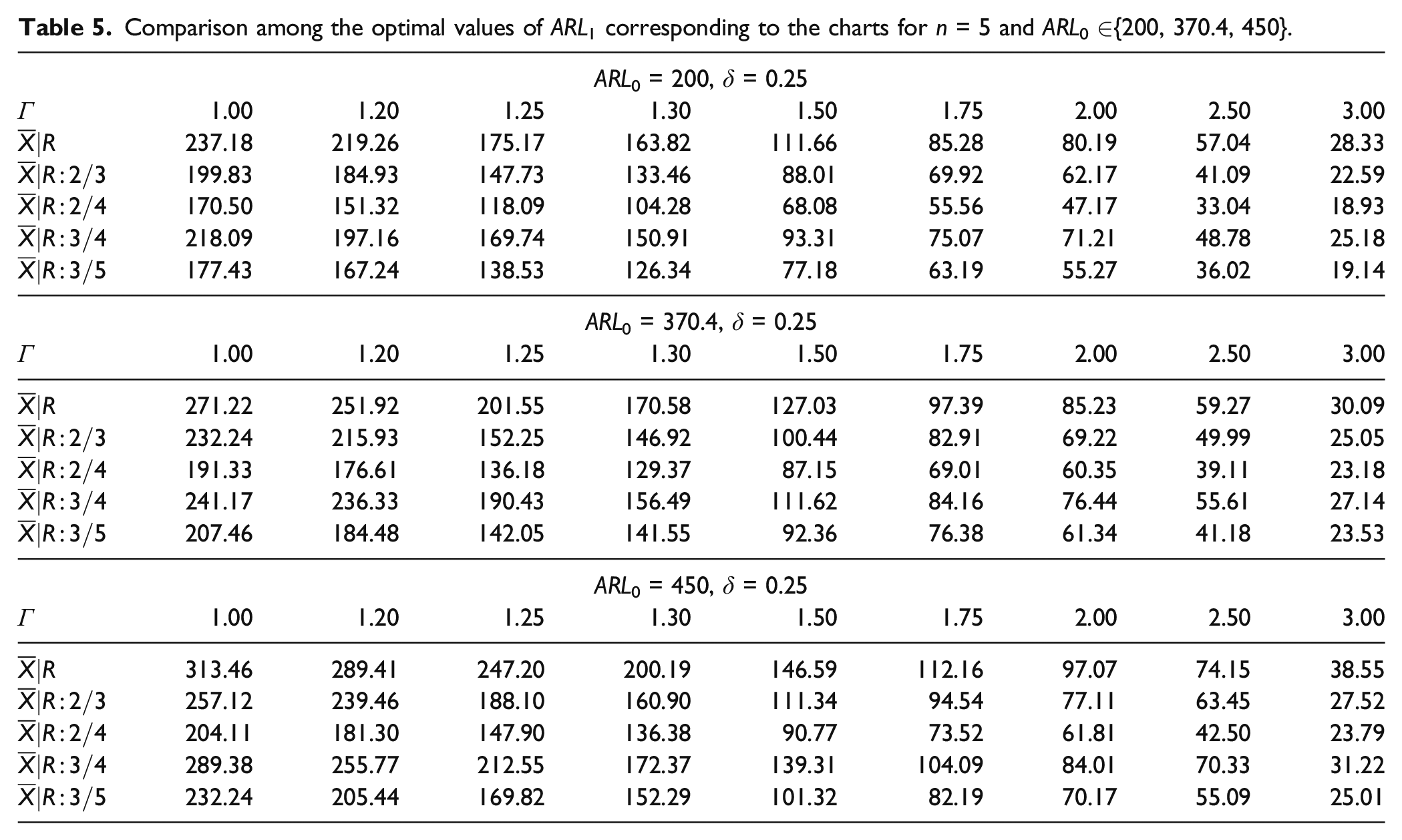
The statistical performances of the charts being considered here have been compared by considering different levels of sample sizes and in-control ARL (ARL ₀) so that the out-of-control ARL (ARL ₁) values of these charts can then be compared for different types of process shifts. To be more specific, the charts, including the conventional $\overline{X}$ and R (denoted by $\overline{X}|R$ ) chart, the EWMA and CUSUM charts, and the joint $\overline{X}|R:r/m$ control chart for m = 3, 4, 5 and m > r > 1, are considered, since these control-chart schemes are frequently used in the literature. For the sake of a fair comparison, the statistical performances of all the considered charts are tested by considering the following constraints: three levels for in-control ARL, ARL ₀ = 200, 370.4, 450 and three levels for the sample size n = 3, 5 and 7. The statistical design of the charts is determined for a wide range of standard deviation shifts between 1 and 3 and a range of process mean shifts between 0 and 0.7.

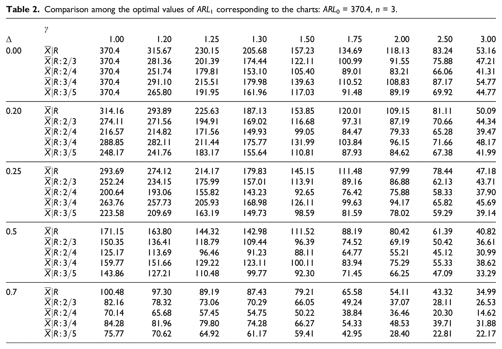
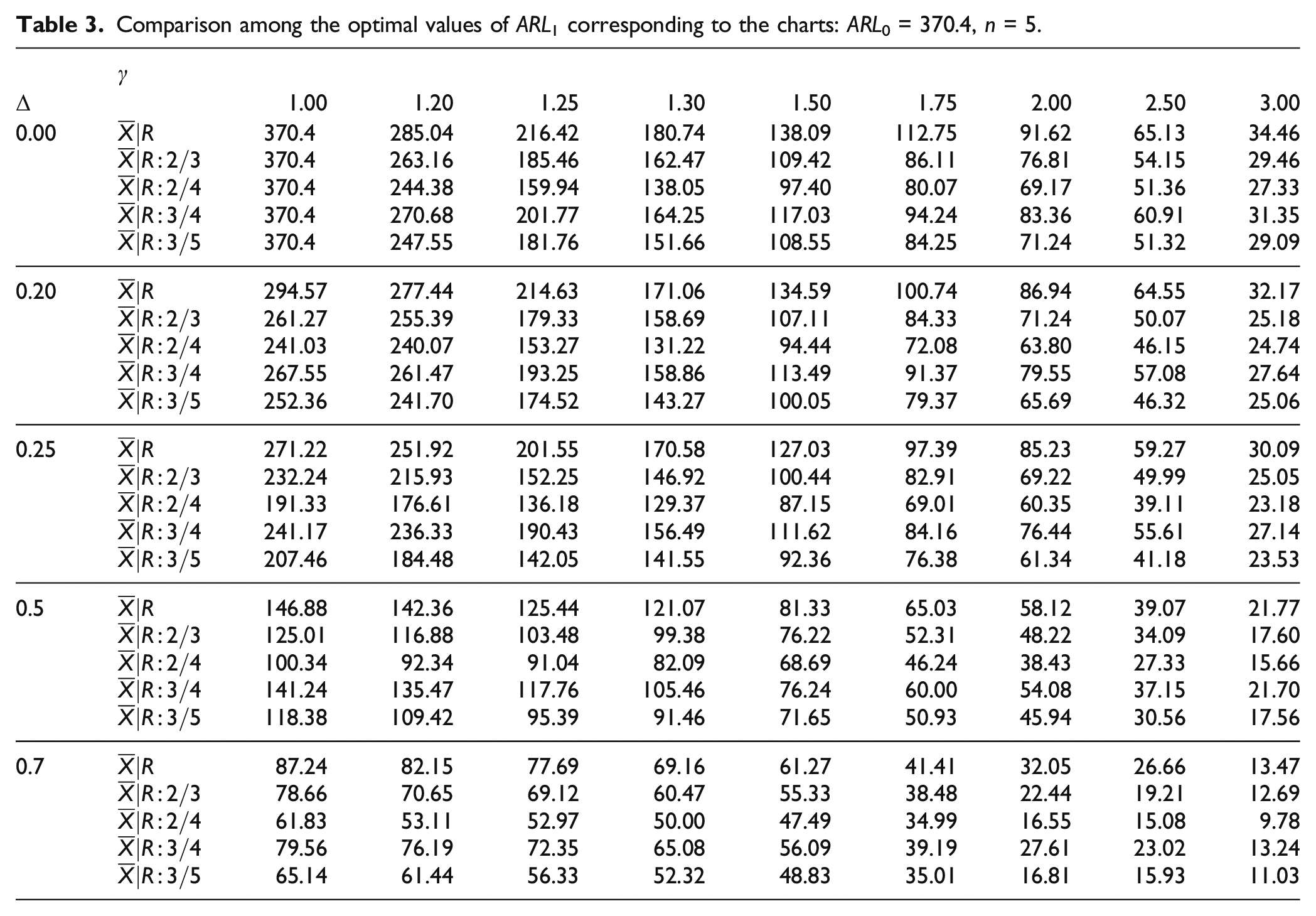
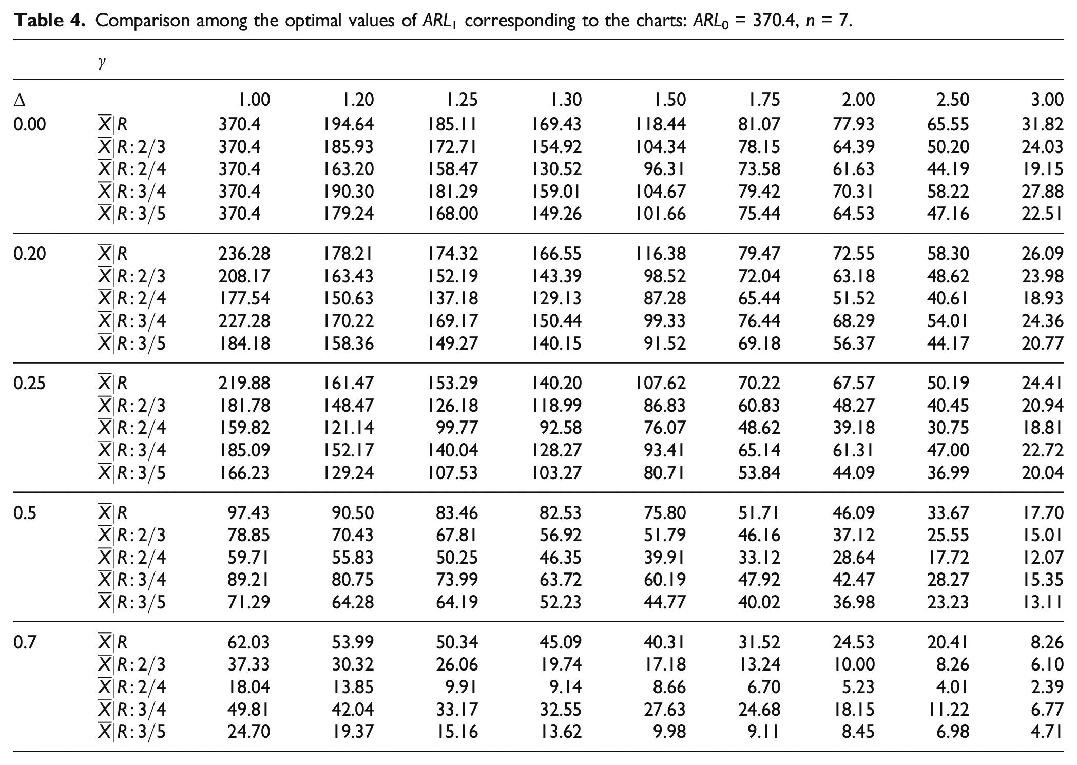
The optimal out-of-control average run length (ARL ₁) for the considered charts are obtained through the developed GA. Tables 2-5 list the achieved results, grouped with respect to the value of sample size and in-control ARL (ARL ₀). Based on the results, it can be concluded that the joint $\overline{X}|R:r/m$ chart always outperforms the conventional $\overline{X}|R$ chart for all different levels of process shifts and various sample size conditions. For example, when ARL ₀ = 370.4, n = 5, the magnitude of the mean shift δ = 0.25 and the magnitude of the standard deviation shift γ = 1.3, the conventional $\overline{X}|R$ scheme needs 170.58 to signal the process change, and the run lengths for $\overline{X}|R:3/4$ , $\overline{X}|R:2/3$ , $\overline{X}|R:3/5$ and $\overline{X}|R:2/4$ schemes to trigger an out-of-control signal are 156.49, 146.92, 141.55 and 129.37, respectively, which indicates the $\overline{X}|R:3/4$ , $\overline{X}|R:2/3$ , $\overline{X}|R:3/5$ and $\overline{X}|R:2/4$ schemes are 8.26%, 13.87%, 17.02% and 24.16% faster than the conventional scheme. It then can be noted that the r out of m runs rules is helpful to enhance the detection ability of the traditional $\overline{X}|R$ control chart.

Table 2.

Comparison among the optimal values of ARL ₁ corresponding to the charts: ARL ₀ = 370.4, n = 3.

	$\gamma$
Δ		1.00	1.20	1.25	1.30	1.50	1.75	2.00	2.50	3.00
0.00	$\overline{X}|R$	370.4	315.67	230.15	205.68	157.23	134.69	118.13	83.24	53.16
	$\overline{X}|R:2/3$	370.4	281.36	201.39	174.44	122.11	100.99	91.55	75.88	47.21
	$\overline{X}|R:2/4$	370.4	251.74	179.81	153.10	105.40	89.01	83.21	66.06	41.31
	$\overline{X}|R:3/4$	370.4	291.10	215.51	179.98	139.63	110.52	108.83	87.17	54.77
	$\overline{X}|R:3/5$	370.4	265.80	191.95	161.96	117.03	91.48	89.19	69.92	44.77
0.20	$\overline{X}|R$	314.16	293.89	225.63	187.13	153.85	120.01	109.15	81.11	50.09
	$\overline{X}|R:2/3$	274.11	271.56	194.91	169.02	116.68	97.31	87.19	70.66	44.34
	$\overline{X}|R:2/4$	216.57	214.82	171.56	149.93	99.05	84.47	79.33	65.28	39.47
	$\overline{X}|R:3/4$	288.85	282.11	211.44	175.77	131.99	103.84	96.15	71.66	48.17
	$\overline{X}|R:3/5$	248.17	241.76	183.17	155.64	110.81	87.93	84.62	67.38	41.99
0.25	$\overline{X}|R$	293.69	274.12	214.17	179.83	145.15	111.48	97.99	78.44	47.18
	$\overline{X}|R:2/3$	252.24	234.15	175.99	157.01	113.91	89.16	86.88	62.13	43.71
	$\overline{X}|R:2/4$	200.64	193.06	155.82	143.23	92.65	76.42	75.88	58.33	37.90
	$\overline{X}|R:3/4$	263.76	257.73	205.93	168.98	126.11	99.63	94.17	65.82	45.69
	$\overline{X}|R:3/5$	223.58	209.69	163.19	149.73	98.59	81.59	78.02	59.29	39.14
0.5	$\overline{X}|R$	171.15	163.80	144.32	142.98	111.52	88.19	80.42	61.39	40.82
	$\overline{X}|R:2/3$	150.35	136.41	118.79	109.44	96.39	74.52	69.19	50.42	36.61
	$\overline{X}|R:2/4$	125.17	113.69	96.46	91.23	88.11	64.77	55.21	45.12	30.99
	$\overline{X}|R:3/4$	159.77	151.66	129.22	123.11	100.11	83.94	75.29	55.33	38.62
	$\overline{X}|R:3/5$	143.86	127.21	110.48	99.77	92.30	71.45	66.25	47.09	33.29
0.7	$\overline{X}|R$	100.48	97.30	89.19	87.43	79.21	65.58	54.11	43.32	34.99
	$\overline{X}|R:2/3$	82.16	78.32	73.06	70.29	66.05	49.24	37.07	28.11	26.53
	$\overline{X}|R:2/4$	70.14	65.68	57.45	54.75	50.22	38.84	36.46	20.30	14.62
	$\overline{X}|R:3/4$	84.28	81.96	79.80	74.28	66.27	54.33	48.53	39.71	31.88
	$\overline{X}|R:3/5$	75.77	70.62	64.92	61.17	59.41	42.95	28.40	22.81	22.17

Table 3.

Comparison among the optimal values of ARL ₁ corresponding to the charts: ARL ₀ = 370.4, n = 5.

	$\gamma$
Δ		1.00	1.20	1.25	1.30	1.50	1.75	2.00	2.50	3.00
0.00	$\overline{X}|R$	370.4	285.04	216.42	180.74	138.09	112.75	91.62	65.13	34.46
	$\overline{X}|R:2/3$	370.4	263.16	185.46	162.47	109.42	86.11	76.81	54.15	29.46
	$\overline{X}|R:2/4$	370.4	244.38	159.94	138.05	97.40	80.07	69.17	51.36	27.33
	$\overline{X}|R:3/4$	370.4	270.68	201.77	164.25	117.03	94.24	83.36	60.91	31.35
	$\overline{X}|R:3/5$	370.4	247.55	181.76	151.66	108.55	84.25	71.24	51.32	29.09
0.20	$\overline{X}|R$	294.57	277.44	214.63	171.06	134.59	100.74	86.94	64.55	32.17
	$\overline{X}|R:2/3$	261.27	255.39	179.33	158.69	107.11	84.33	71.24	50.07	25.18
	$\overline{X}|R:2/4$	241.03	240.07	153.27	131.22	94.44	72.08	63.80	46.15	24.74
	$\overline{X}|R:3/4$	267.55	261.47	193.25	158.86	113.49	91.37	79.55	57.08	27.64
	$\overline{X}|R:3/5$	252.36	241.70	174.52	143.27	100.05	79.37	65.69	46.32	25.06
0.25	$\overline{X}|R$	271.22	251.92	201.55	170.58	127.03	97.39	85.23	59.27	30.09
	$\overline{X}|R:2/3$	232.24	215.93	152.25	146.92	100.44	82.91	69.22	49.99	25.05
	$\overline{X}|R:2/4$	191.33	176.61	136.18	129.37	87.15	69.01	60.35	39.11	23.18
	$\overline{X}|R:3/4$	241.17	236.33	190.43	156.49	111.62	84.16	76.44	55.61	27.14
	$\overline{X}|R:3/5$	207.46	184.48	142.05	141.55	92.36	76.38	61.34	41.18	23.53
0.5	$\overline{X}|R$	146.88	142.36	125.44	121.07	81.33	65.03	58.12	39.07	21.77
	$\overline{X}|R:2/3$	125.01	116.88	103.48	99.38	76.22	52.31	48.22	34.09	17.60
	$\overline{X}|R:2/4$	100.34	92.34	91.04	82.09	68.69	46.24	38.43	27.33	15.66
	$\overline{X}|R:3/4$	141.24	135.47	117.76	105.46	76.24	60.00	54.08	37.15	21.70
	$\overline{X}|R:3/5$	118.38	109.42	95.39	91.46	71.65	50.93	45.94	30.56	17.56
0.7	$\overline{X}|R$	87.24	82.15	77.69	69.16	61.27	41.41	32.05	26.66	13.47
	$\overline{X}|R:2/3$	78.66	70.65	69.12	60.47	55.33	38.48	22.44	19.21	12.69
	$\overline{X}|R:2/4$	61.83	53.11	52.97	50.00	47.49	34.99	16.55	15.08	9.78
	$\overline{X}|R:3/4$	79.56	76.19	72.35	65.08	56.09	39.19	27.61	23.02	13.24
	$\overline{X}|R:3/5$	65.14	61.44	56.33	52.32	48.83	35.01	16.81	15.93	11.03

Table 4.

Comparison among the optimal values of ARL ₁ corresponding to the charts: ARL ₀ = 370.4, n = 7.

	$\gamma$
Δ		1.00	1.20	1.25	1.30	1.50	1.75	2.00	2.50	3.00
0.00	$\overline{X}|R$	370.4	194.64	185.11	169.43	118.44	81.07	77.93	65.55	31.82
	$\overline{X}|R:2/3$	370.4	185.93	172.71	154.92	104.34	78.15	64.39	50.20	24.03
	$\overline{X}|R:2/4$	370.4	163.20	158.47	130.52	96.31	73.58	61.63	44.19	19.15
	$\overline{X}|R:3/4$	370.4	190.30	181.29	159.01	104.67	79.42	70.31	58.22	27.88
	$\overline{X}|R:3/5$	370.4	179.24	168.00	149.26	101.66	75.44	64.53	47.16	22.51
0.20	$\overline{X}|R$	236.28	178.21	174.32	166.55	116.38	79.47	72.55	58.30	26.09
	$\overline{X}|R:2/3$	208.17	163.43	152.19	143.39	98.52	72.04	63.18	48.62	23.98
	$\overline{X}|R:2/4$	177.54	150.63	137.18	129.13	87.28	65.44	51.52	40.61	18.93
	$\overline{X}|R:3/4$	227.28	170.22	169.17	150.44	99.33	76.44	68.29	54.01	24.36
	$\overline{X}|R:3/5$	184.18	158.36	149.27	140.15	91.52	69.18	56.37	44.17	20.77
0.25	$\overline{X}|R$	219.88	161.47	153.29	140.20	107.62	70.22	67.57	50.19	24.41
	$\overline{X}|R:2/3$	181.78	148.47	126.18	118.99	86.83	60.83	48.27	40.45	20.94
	$\overline{X}|R:2/4$	159.82	121.14	99.77	92.58	76.07	48.62	39.18	30.75	18.81
	$\overline{X}|R:3/4$	185.09	152.17	140.04	128.27	93.41	65.14	61.31	47.00	22.72
	$\overline{X}|R:3/5$	166.23	129.24	107.53	103.27	80.71	53.84	44.09	36.99	20.04
0.5	$\overline{X}|R$	97.43	90.50	83.46	82.53	75.80	51.71	46.09	33.67	17.70
	$\overline{X}|R:2/3$	78.85	70.43	67.81	56.92	51.79	46.16	37.12	25.55	15.01
	$\overline{X}|R:2/4$	59.71	55.83	50.25	46.35	39.91	33.12	28.64	17.72	12.07
	$\overline{X}|R:3/4$	89.21	80.75	73.99	63.72	60.19	47.92	42.47	28.27	15.35
	$\overline{X}|R:3/5$	71.29	64.28	64.19	52.23	44.77	40.02	36.98	23.23	13.11
0.7	$\overline{X}|R$	62.03	53.99	50.34	45.09	40.31	31.52	24.53	20.41	8.26
	$\overline{X}|R:2/3$	37.33	30.32	26.06	19.74	17.18	13.24	10.00	8.26	6.10
	$\overline{X}|R:2/4$	18.04	13.85	9.91	9.14	8.66	6.70	5.23	4.01	2.39
	$\overline{X}|R:3/4$	49.81	42.04	33.17	32.55	27.63	24.68	18.15	11.22	6.77
	$\overline{X}|R:3/5$	24.70	19.37	15.16	13.62	9.98	9.11	8.45	6.98	4.71

Table 5.

Comparison among the optimal values of ARL ₁ corresponding to the charts for n = 5 and ARL ₀ ∈{200, 370.4, 450}.

ARL 0 = 200, δ = 0.25
Γ	1.00	1.20	1.25	1.30	1.50	1.75	2.00	2.50	3.00
$\overline{X}|R$	237.18	219.26	175.17	163.82	111.66	85.28	80.19	57.04	28.33
$\overline{X}|R:2/3$	199.83	184.93	147.73	133.46	88.01	69.92	62.17	41.09	22.59
$\overline{X}|R:2/4$	170.50	151.32	118.09	104.28	68.08	55.56	47.17	33.04	18.93
$\overline{X}|R:3/4$	218.09	197.16	169.74	150.91	93.31	75.07	71.21	48.78	25.18
$\overline{X}|R:3/5$	177.43	167.24	138.53	126.34	77.18	63.19	55.27	36.02	19.14
ARL 0 = 370.4, δ = 0.25
Γ	1.00	1.20	1.25	1.30	1.50	1.75	2.00	2.50	3.00
$\overline{X}|R$	271.22	251.92	201.55	170.58	127.03	97.39	85.23	59.27	30.09
$\overline{X}|R:2/3$	232.24	215.93	152.25	146.92	100.44	82.91	69.22	49.99	25.05
$\overline{X}|R:2/4$	191.33	176.61	136.18	129.37	87.15	69.01	60.35	39.11	23.18
$\overline{X}|R:3/4$	241.17	236.33	190.43	156.49	111.62	84.16	76.44	55.61	27.14
$\overline{X}|R:3/5$	207.46	184.48	142.05	141.55	92.36	76.38	61.34	41.18	23.53
ARL 0 = 450, δ = 0.25
Γ	1.00	1.20	1.25	1.30	1.50	1.75	2.00	2.50	3.00
$\overline{X}|R$	313.46	289.41	247.20	200.19	146.59	112.16	97.07	74.15	38.55
$\overline{X}|R:2/3$	257.12	239.46	188.10	160.90	111.34	94.54	77.11	63.45	27.52
$\overline{X}|R:2/4$	204.11	181.30	147.90	136.38	90.77	73.52	61.81	42.50	23.79
$\overline{X}|R:3/4$	289.38	255.77	212.55	172.37	139.31	104.09	84.01	70.33	31.22
$\overline{X}|R:3/5$	232.24	205.44	169.82	152.29	101.32	82.19	70.17	55.09	25.01

Based on the results of Tables 2 and 3, we also conclude that, in terms of the ARL ₁, the 2/4 runs-rules scheme is superior to the 3/5 scheme, the 3/5 scheme is superior to the 2/3 scheme and the 2/3 scheme is superior to the 3/4 scheme. This is because depending on the selection of specific values of r and m, the control chart adopting a more strict detection standard tends to signal an out-of-control signal more timely. For example, according to the definition of the r out of m runs rules, the 2/4 scheme triggers an alarm as long as two sample points fall within the warning region, while the 3/4 scheme needs three. It indicates that the 2/4 scheme adopted a more strict detection standard than the 3/4 scheme.

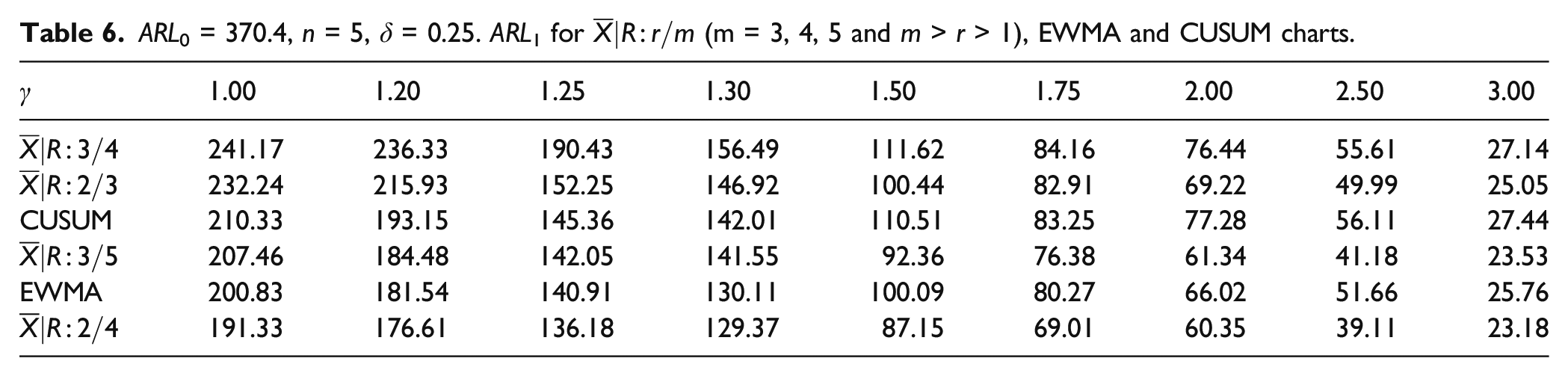
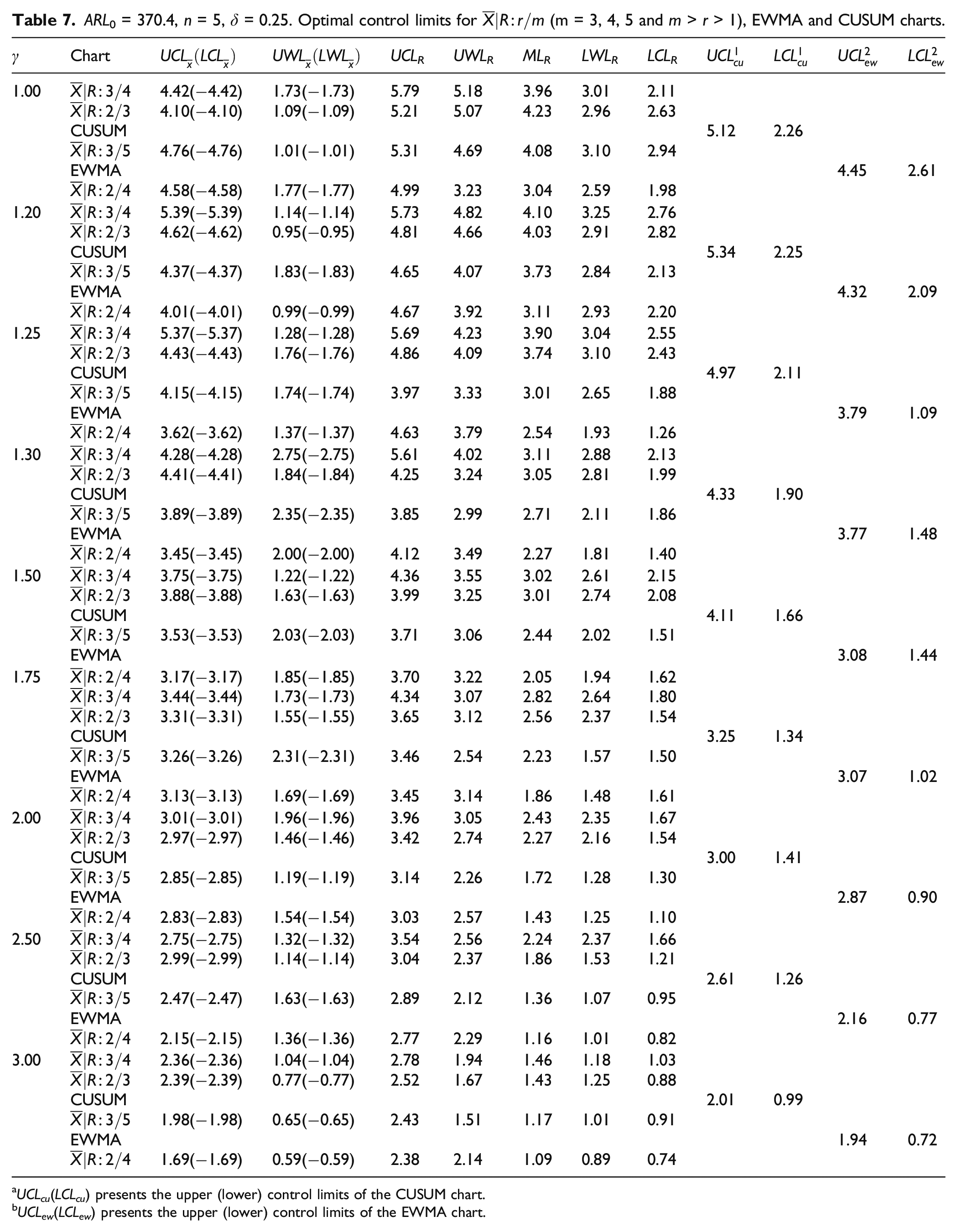
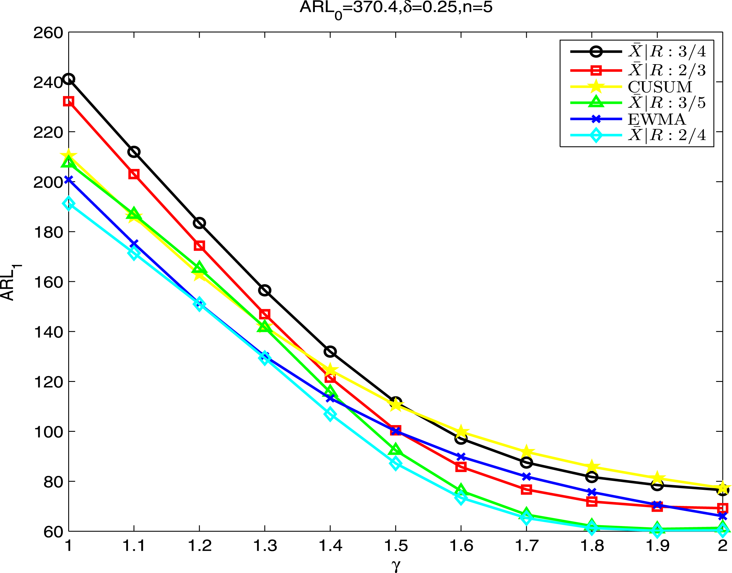
A comparison with EWMA and CUSUM control charts is also investigated and the results are shown in Table 6. Table 7 presents the corresponding optimal control limits for all the charts considered in Table 6. The obtained results indicate that the suggested chart performs better than the EWMA and CUSUM charts in detecting large process fluctuations. Moreover, the performance of the proposed scheme for detecting small shifts is close to or even better than that of its competitors when specific values of r and m are selected. This behaviour is graphically shown in Figure 3.

Table 6.

ARL ₀ = 370.4, n = 5, δ = 0.25. ARL ₁ for $\overline{X}|R:r/m$ (m = 3, 4, 5 and m > r > 1), EWMA and CUSUM charts.

γ	1.00	1.20	1.25	1.30	1.50	1.75	2.00	2.50	3.00
$\overline{X}|R:3/4$	241.17	236.33	190.43	156.49	111.62	84.16	76.44	55.61	27.14
$\overline{X}|R:2/3$	232.24	215.93	152.25	146.92	100.44	82.91	69.22	49.99	25.05
CUSUM	210.33	193.15	145.36	142.01	110.51	83.25	77.28	56.11	27.44
$\overline{X}|R:3/5$	207.46	184.48	142.05	141.55	92.36	76.38	61.34	41.18	23.53
EWMA	200.83	181.54	140.91	130.11	100.09	80.27	66.02	51.66	25.76
$\overline{X}|R:2/4$	191.33	176.61	136.18	129.37	87.15	69.01	60.35	39.11	23.18

Table 7.

ARL ₀ = 370.4, n = 5, δ = 0.25. Optimal control limits for $\overline{X}|R:r/m$ (m = 3, 4, 5 and m > r > 1), EWMA and CUSUM charts.

γ	Chart	$UC{L}_{\overline{x}}\left(LC{L}_{\overline{x}}\right)$	$UW{L}_{\overline{x}}\left(LW{L}_{\overline{x}}\right)$	UCL R	UWL R	ML R	LWL R	LCL R	$UC{L}_{cu}^1$	$LC{L}_{cu}^1$	$UC{L}_{ew}^2$	$LC{L}_{ew}^2$
1.00	$\overline{X}|R:3/4$	4.42(−4.42)	1.73(−1.73)	5.79	5.18	3.96	3.01	2.11
	$\overline{X}|R:2/3$	4.10(−4.10)	1.09(−1.09)	5.21	5.07	4.23	2.96	2.63
	CUSUM								5.12	2.26
	$\overline{X}|R:3/5$	4.76(−4.76)	1.01(−1.01)	5.31	4.69	4.08	3.10	2.94
	EWMA										4.45	2.61
	$\overline{X}|R:2/4$	4.58(−4.58)	1.77(−1.77)	4.99	3.23	3.04	2.59	1.98
1.20	$\overline{X}|R:3/4$	5.39(−5.39)	1.14(−1.14)	5.73	4.82	4.10	3.25	2.76
	$\overline{X}|R:2/3$	4.62(−4.62)	0.95(−0.95)	4.81	4.66	4.03	2.91	2.82
	CUSUM								5.34	2.25
	$\overline{X}|R:3/5$	4.37(−4.37)	1.83(−1.83)	4.65	4.07	3.73	2.84	2.13
	EWMA										4.32	2.09
	$\overline{X}|R:2/4$	4.01(−4.01)	0.99(−0.99)	4.67	3.92	3.11	2.93	2.20
1.25	$\overline{X}|R:3/4$	5.37(−5.37)	1.28(−1.28)	5.69	4.23	3.90	3.04	2.55
	$\overline{X}|R:2/3$	4.43(−4.43)	1.76(−1.76)	4.86	4.09	3.74	3.10	2.43
	CUSUM								4.97	2.11
	$\overline{X}|R:3/5$	4.15(−4.15)	1.74(−1.74)	3.97	3.33	3.01	2.65	1.88
	EWMA										3.79	1.09
	$\overline{X}|R:2/4$	3.62(−3.62)	1.37(−1.37)	4.63	3.79	2.54	1.93	1.26
1.30	$\overline{X}|R:3/4$	4.28(−4.28)	2.75(−2.75)	5.61	4.02	3.11	2.88	2.13
	$\overline{X}|R:2/3$	4.41(−4.41)	1.84(−1.84)	4.25	3.24	3.05	2.81	1.99
	CUSUM								4.33	1.90
	$\overline{X}|R:3/5$	3.89(−3.89)	2.35(−2.35)	3.85	2.99	2.71	2.11	1.86
	EWMA										3.77	1.48
	$\overline{X}|R:2/4$	3.45(−3.45)	2.00(−2.00)	4.12	3.49	2.27	1.81	1.40
1.50	$\overline{X}|R:3/4$	3.75(−3.75)	1.22(−1.22)	4.36	3.55	3.02	2.61	2.15
	$\overline{X}|R:2/3$	3.88(−3.88)	1.63(−1.63)	3.99	3.25	3.01	2.74	2.08
	CUSUM								4.11	1.66
	$\overline{X}|R:3/5$	3.53(−3.53)	2.03(−2.03)	3.71	3.06	2.44	2.02	1.51
	EWMA										3.08	1.44
1.75	$\overline{X}|R:2/4$	3.17(−3.17)	1.85(−1.85)	3.70	3.22	2.05	1.94	1.62
	$\overline{X}|R:3/4$	3.44(−3.44)	1.73(−1.73)	4.34	3.07	2.82	2.64	1.80
	$\overline{X}|R:2/3$	3.31(−3.31)	1.55(−1.55)	3.65	3.12	2.56	2.37	1.54
	CUSUM								3.25	1.34
	$\overline{X}|R:3/5$	3.26(−3.26)	2.31(−2.31)	3.46	2.54	2.23	1.57	1.50
	EWMA										3.07	1.02
	$\overline{X}|R:2/4$	3.13(−3.13)	1.69(−1.69)	3.45	3.14	1.86	1.48	1.61
2.00	$\overline{X}|R:3/4$	3.01(−3.01)	1.96(−1.96)	3.96	3.05	2.43	2.35	1.67
	$\overline{X}|R:2/3$	2.97(−2.97)	1.46(−1.46)	3.42	2.74	2.27	2.16	1.54
	CUSUM								3.00	1.41
	$\overline{X}|R:3/5$	2.85(−2.85)	1.19(−1.19)	3.14	2.26	1.72	1.28	1.30
	EWMA										2.87	0.90
	$\overline{X}|R:2/4$	2.83(−2.83)	1.54(−1.54)	3.03	2.57	1.43	1.25	1.10
2.50	$\overline{X}|R:3/4$	2.75(−2.75)	1.32(−1.32)	3.54	2.56	2.24	2.37	1.66
	$\overline{X}|R:2/3$	2.99(−2.99)	1.14(−1.14)	3.04	2.37	1.86	1.53	1.21
	CUSUM								2.61	1.26
	$\overline{X}|R:3/5$	2.47(−2.47)	1.63(−1.63)	2.89	2.12	1.36	1.07	0.95
	EWMA										2.16	0.77
	$\overline{X}|R:2/4$	2.15(−2.15)	1.36(−1.36)	2.77	2.29	1.16	1.01	0.82
3.00	$\overline{X}|R:3/4$	2.36(−2.36)	1.04(−1.04)	2.78	1.94	1.46	1.18	1.03
	$\overline{X}|R:2/3$	2.39(−2.39)	0.77(−0.77)	2.52	1.67	1.43	1.25	0.88
	CUSUM								2.01	0.99
	$\overline{X}|R:3/5$	1.98(−1.98)	0.65(−0.65)	2.43	1.51	1.17	1.01	0.91
	EWMA										1.94	0.72
	$\overline{X}|R:2/4$	1.69(−1.69)	0.59(−0.59)	2.38	2.14	1.09	0.89	0.74

^a UCL _cu (LCL _cu ) presents the upper (lower) control limits of the CUSUM chart.

^b UCL _ew (LCL _ew ) presents the upper (lower) control limits of the EWMA chart.

Figure 3.

Comparison among different control-chart schemes.

Effects of parameters on ARL ₁

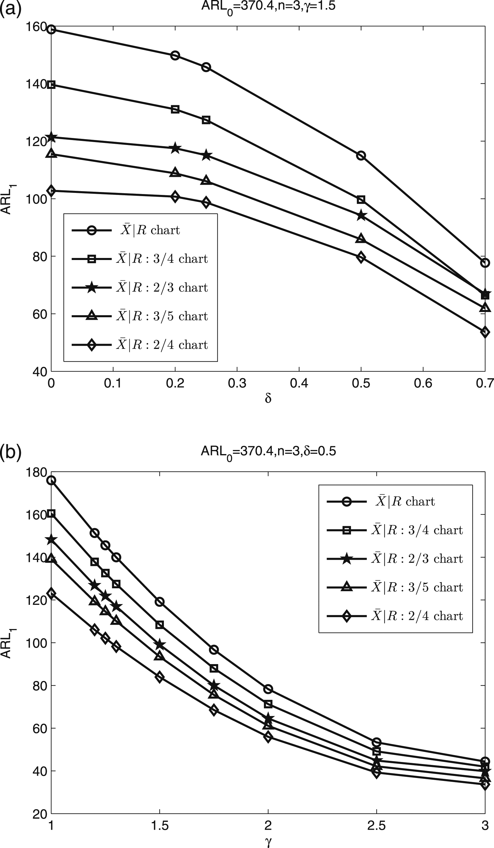
In the previous section, we found that the joint $\overline{X}|R:r/m$ chart is better than the traditional $\overline{X}|R$ chart in terms of ARL ₁. The established control-chart model achieved ARL ₁-saving compared to the conventional $\overline{X}|R$ without r out of m runs rules. Nonetheless, according to Figures 4 and 5, it is found that the improvement varies with different values of key parameters (including δ, γ, n and ARL ₀). The main results are summarized as follows.

Figure 4.

Effects of δ and γ over the out-of-control average run length ARL ₁.

Figure 5.

Effects of n and ARL ₀ on the out-of-control average run length ARL ₁.

Figure 4 shows that as the magnitude of the process mean (standard deviation) shift grows, the ARL ₁ of all the considered chart decrease. This is because when the process possesses a larger shift in the mean (standard deviation), the control chart needs a shorter time to trigger an out-of-control signal. Furthermore, we found that the chart with r out of m runs rules has a larger statistical performance improvement than the chart without runs rules in detecting small-to-moderate process shifts. As expected, when the magnitude of the process shift increases to a certain level, all the considered charts have similar statistical performance.

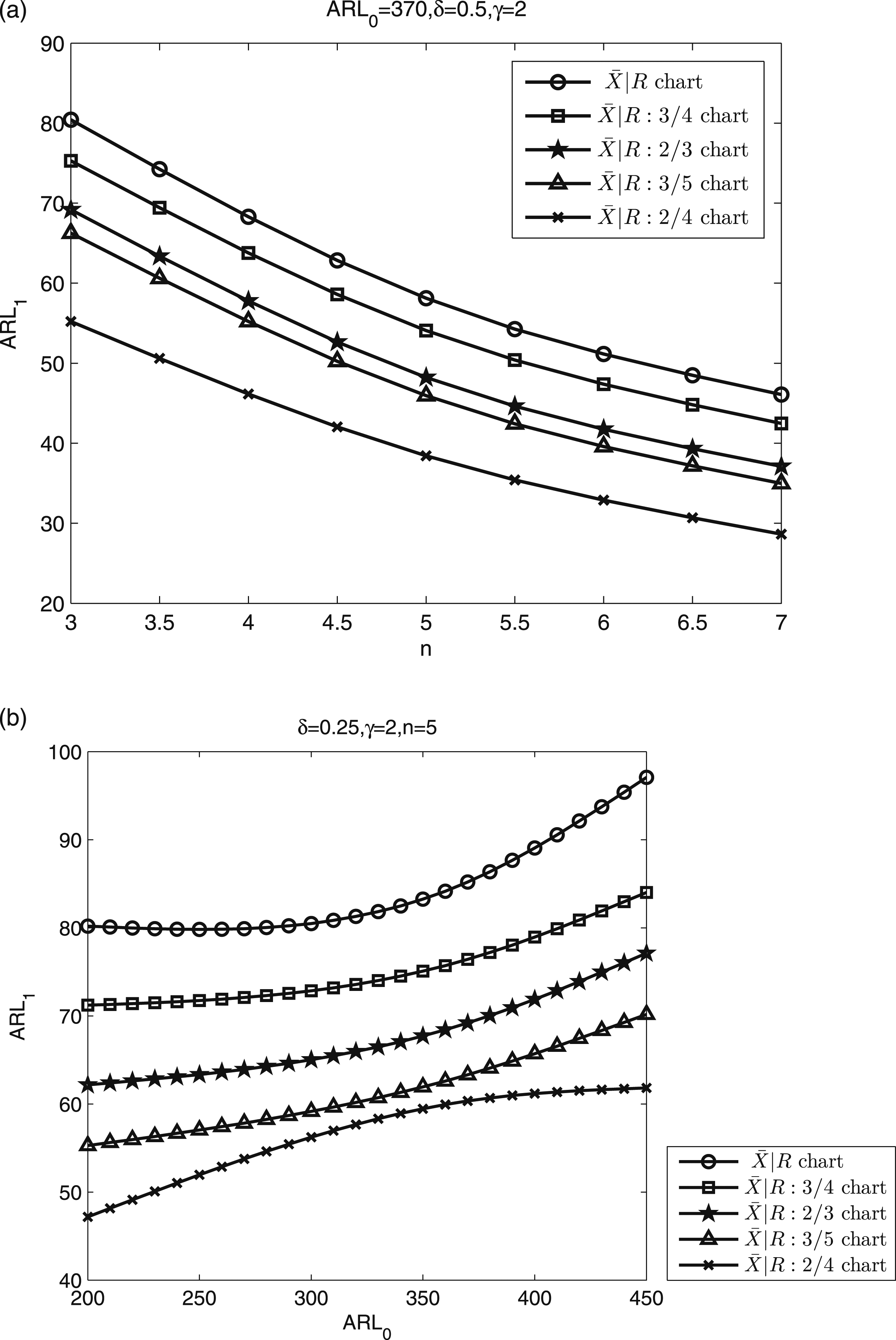
It follows from Figure 5(a) that with the increase of sample size n, the ARL ₁ for all the considered charts decreases. For instance, for detecting a specific process shift (δ = 0.5 and γ = 2), the $\overline{X}|R:2/4$ chart with n = 3 needs ARL ₁ = 55.21 to signal an out-of-control process, while the ARL ₁ for the corresponding chart with n = 7 to trigger an out-of-control signal is 28.64, which indicates that the $\overline{X}|R:2/4$ chart with n = 7 is 48.13% faster than the corresponding chart with n = 3. This could be because the control chart with a larger sample size can collect more information about the process so that the out-of-control situation can be signalled more timely. Still investigating Figure 5(a), it is found that, on average, with the increase of n, for fixed δ and γ, the difference between the ARL ₁ values corresponding to the charts considered decreases. For example, when δ = 0.5, γ = 2 and n = 3, the ARL ₁ for $\overline{X}|R:2/3$ and $\overline{X}|R:2/4$ schemes are, respectively, 69.19 and 55.21, which indicates the 2/4 runs-rules scheme is 20.21% faster than the 2/4 runs-rules scheme. But when the sample size n = 5 is considered and the other parameters remain the same, the ARL ₁ for $\overline{X}|R:2/3$ and $\overline{X}|R:2/4$ schemes are, respectively, 34.09 and 27.33, which indicates the 2/4 runs-rules scheme is 19.83% faster than the 2/4 runs-rules scheme in this situation. Additionally, it is worth noting that, due to the fact that the developed GA cannot always obtain the global optimal solution, as n increases, the difference between the ARL ₁ values corresponding to the charts considered may increase in several cases. But overall, for all the charts considered, as n increases, the effect of the increase of sample size on ARL ₁ becomes disappearing.

Figure 5(b) illustrates that the larger the in-control ARL ARL ₀, the larger the out-of-control ARL ARL ₁. This may be explained by the fact that when a larger ARL ₀ is designed, the chart tends to have a more relaxed control-limit scheme. It then leads to the result that the more time needed by the chart to trigger a signal when a process shift occurs.

Effects of parameter estimation on ARL ₁

In the application of control charts, the mean and/or the variance of a production/service process are usually unknown. Therefore, before the control charts can be put to good use, one or both of the parameters should be pre-estimated. Undoubtedly, when estimates are employed as a substitute for known parameter values, the statistical properties of the chart considered can be greatly affected. Thus, in the process of application of control charts, the effects of parameter estimation should be clearly assessed and properly accounted for.

In general, parameter estimation can be divided into three cases: mean unknown but variance known, mean known but variance unknown and mean and variance both unknown. In our model, when the variance ${\sigma }_0^2$ is unspecified and estimated from Phase I reference data, the cumulative distribution function for W ₀ as shown in equation (7) will be completely changed, which makes it too complex to analyse the properties of the R sub-chart mathematically. Therefore, in this subsection, we only focus on the first case, that is, mean unknown but variance known.

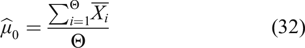
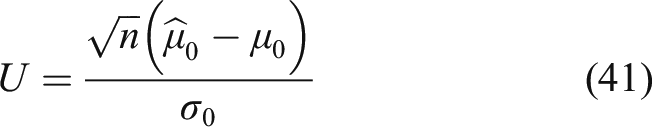
In order to obtain the estimator for the in-control process mean μ ₀, Θ subgroups of size n are sampled from Phase I. Denote the grand mean of those Θ subgroups by ${\widehat{\mu }}_0$ . Then, μ ₀ can be estimated by the estimator below

$${\widehat{\mu }}_0=\frac{{\displaystyle {\sum }_{i=1}^{\mathrm{\Theta }}\overline{X_i}}}{\mathrm{\Theta }}$$

(32)

where $\overline{X_i}$ is the mean of the i ^th subgroup, i = 1, 2, ‥, Θ. Then, in the parameter-estimation case, the control limits of $\overline{X}$ sub-chart can be rewritten as

$${\widehat{UCL}}_{\overline{X}}={\widehat{\mu }}_0+{\widehat{k}}_1\frac{{\sigma }_0}{\sqrt{n}}, {\widehat{UWL}}_{\overline{X}}={\widehat{\mu }}_0+{\widehat{k}}_2\frac{{\sigma }_0}{\sqrt{n}}$$

(33)

$${\widehat{LWL}}_{\overline{X}}={\widehat{\mu }}_0-{\widehat{k}}_2\frac{{\sigma }_0}{\sqrt{n}}, {\widehat{LCL}}_{\overline{X}}={\widehat{\mu }}_0-{\widehat{k}}_1\frac{{\sigma }_0}{\sqrt{n}}$$

(34)

where ${\widehat{k}}_1$ and ${\widehat{k}}_2$ ( ${\widehat{k}}_1\ge {\widehat{k}}_2$ ) are the control limit coefficients.

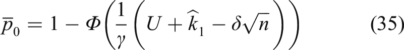
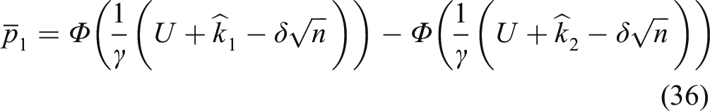
In such condition, let ${\overline{p}}_0$ , ${\overline{p}}_1$ , ${\overline{p}}_2$ , ${\overline{p}}_3$ , ${\overline{p}}_4$ and ${\overline{p}}_5$ denote the probability that a mean point falls in regions 0, 1, 2, 3, 4 and 5, respectively. Then, we have

$${\overline{p}}_0=1-\Phi \left(\frac{1}{\gamma }\left(U+{\widehat{k}}_1-\delta \sqrt{n}\right)\right)$$

(35)

$${\overline{p}}_1=\Phi \left(\frac{1}{\gamma }\left(U+{\widehat{k}}_1-\delta \sqrt{n}\right)\right)-\Phi \left(\frac{1}{\gamma }\left(U+{\widehat{k}}_2-\delta \sqrt{n}\right)\right)$$

(36)

$${\overline{p}}_2=\Phi \left(\frac{1}{\gamma }\left(U+{\widehat{k}}_2-\delta \sqrt{n}\right)\right)-\Phi \left(\frac{1}{\gamma }\left(U-\delta \sqrt{n}\right)\right)$$

(37)

$${\overline{p}}_3=\Phi \left(\frac{1}{\gamma }\left(U-\delta \sqrt{n}\right)\right)-\Phi \left(\frac{1}{\gamma }\left(U-{\widehat{k}}_2-\delta \sqrt{n}\right)\right)$$

(38)

$${\overline{p}}_4=\Phi \left(\frac{1}{\gamma }\left(U-{\widehat{k}}_2-\delta \sqrt{n}\right)\right)-\Phi \left(\frac{1}{\gamma }\left(U-{\widehat{k}}_1-\delta \sqrt{n}\right)\right)$$

(39)

$${\overline{p}}_5=\Phi \left(\frac{1}{\gamma }\left(U-{\widehat{k}}_1-\delta \sqrt{n}\right)\right)$$

(40)

where

$$U=\frac{\sqrt{n}\left({\widehat{\mu }}_0-{\mu }_0\right)}{{\sigma }_0}$$

(41)

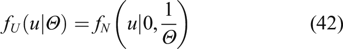
Because ${\widehat{\mu }}_0$ is a normal random variable with mean μ ₀ and variance ${\sigma }_0^2/\Theta n$ , we then have ${\widehat{\mu }}_0\sim N\left({\mu }_0,{\sigma }_0^2/\Theta n\right)$ and $U\sim N\left(0,1/\Theta \right)$ . The probability density function (PDF) of U can then be written as

$$f_U\left(u|\Theta \right)=f_N\left(u|0,\frac{1}{\Theta }\right)$$

(42)

where $f_N\left(u|0,1/\Theta \right)$ is the PDF of the normal distribution with mean 0 and variance $1/\Theta$ .

Due to the difficulties in deriving the general formulate of ARL for the study of the $\overline{X}|R:r/m$ chart, in this subsection, the $\overline{X}|R:2/4$ scheme will still be studied as a typical instance of the whole class of $\overline{X}|R:r/m$ chart. It is easy to find that compared to the known-parameter case, only the calculation of ARL for the $\overline{X}|R:r/m$ sub-chart has changed and the rest remains the same in the estimated-parameter case.

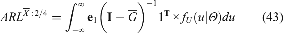
The unconditional ARL of the $\overline{X}:2/4$ sub-chart in the estimated-parameter case then can be given by

$$AR{L}^{\overline{X}:2/4}={\displaystyle {\int }_{-\infty }^{\infty }{\mathbf{e}}_{\mathrm{1}}{\left(\mathbf{I}-\overline{G}\right)}^{-\mathrm{1}}{\mathrm{1}}^{\mathbf{T}}\times f_U\left(u|\Theta \right)du}$$

(43)

where $\overline{G}$ is the matrix G in which the probabilities p _i (i = 0, 1, 2, 3, 4, 5) are replaced by ${\overline{p}}_i\left(i=\mathrm{0,1,2,3,4,5}\right)$ .

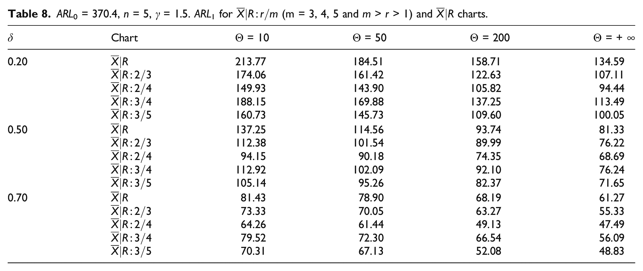
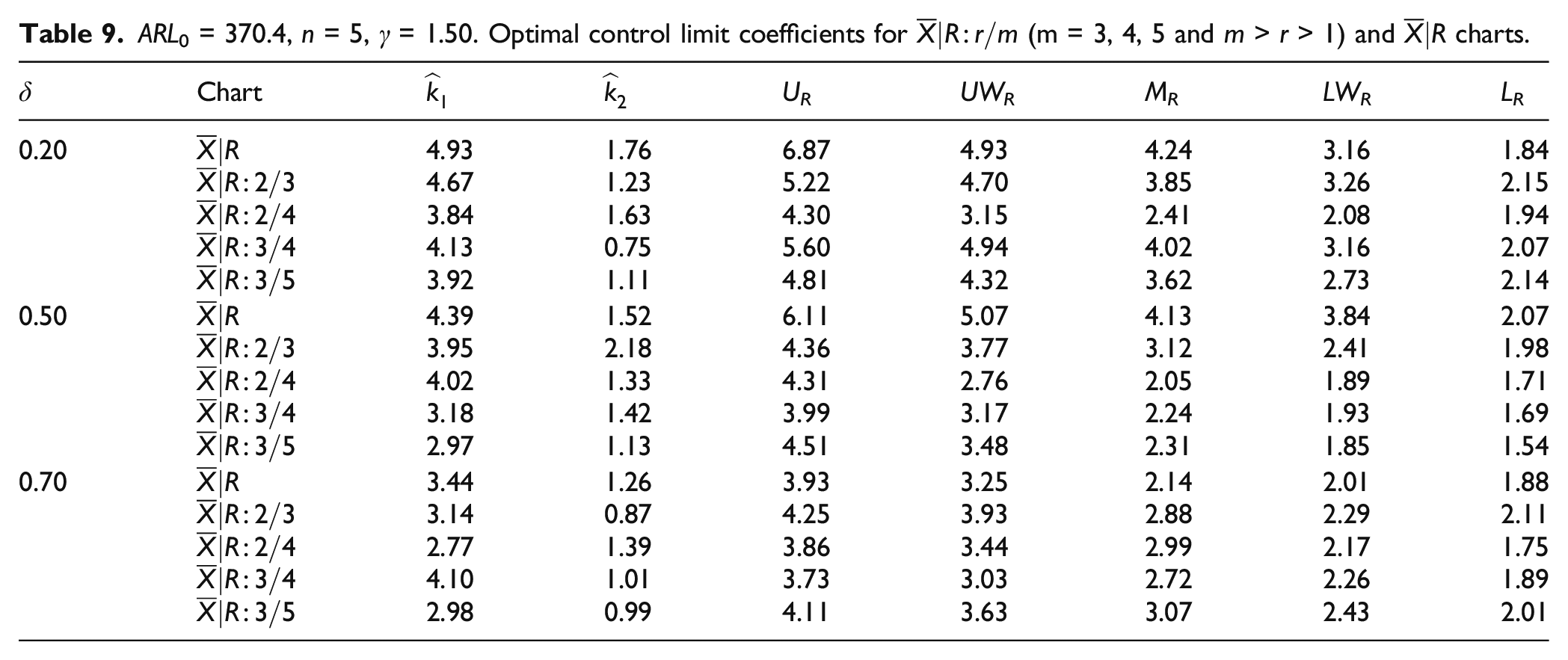
Next, a numerical analysis is conducted to investigate the effects of parameter estimation on $..$ charts based on the out-of-control ARL (ARL ₁). By employing different combinations of the number of subgroups Θ = 10, 50, 200, + ∞, the magnitude of the shift in the standard deviation γ = 1.5, the in-control ARL ARL ₀=370.4 and the sample size n = 5, the optimal ARL ₁ values are obtained by using the developed GA and presented in Table 8. The extreme case of Θ = + ∞ represents the known-parameter case and the other Θ values represent the estimated-parameter cases. Table 9 lists the optimal control limit coefficients for the charts corresponding to the cases in Table 8.

Table 8.

ARL ₀ = 370.4, n = 5, γ = 1.5. ARL ₁ for $\overline{X}|R:r/m$ (m = 3, 4, 5 and m > r > 1) and $\overline{X}|R$ charts.

δ	Chart	Θ = 10	Θ = 50	Θ = 200	Θ = + ∞
0.20	$\overline{X}|R$	213.77	184.51	158.71	134.59
	$\overline{X}|R:2/3$	174.06	161.42	122.63	107.11
	$\overline{X}|R:2/4$	149.93	143.90	105.82	94.44
	$\overline{X}|R:3/4$	188.15	169.88	137.25	113.49
	$\overline{X}|R:3/5$	160.73	145.73	109.60	100.05
0.50	$\overline{X}|R$	137.25	114.56	93.74	81.33
	$\overline{X}|R:2/3$	112.38	101.54	89.99	76.22
	$\overline{X}|R:2/4$	94.15	90.18	74.35	68.69
	$\overline{X}|R:3/4$	112.92	102.09	92.10	76.24
	$\overline{X}|R:3/5$	105.14	95.26	82.37	71.65
0.70	$\overline{X}|R$	81.43	78.90	68.19	61.27
	$\overline{X}|R:2/3$	73.33	70.05	63.27	55.33
	$\overline{X}|R:2/4$	64.26	61.44	49.13	47.49
	$\overline{X}|R:3/4$	79.52	72.30	66.54	56.09
	$\overline{X}|R:3/5$	70.31	67.13	52.08	48.83

Table 9.

ARL ₀ = 370.4, n = 5, γ = 1.50. Optimal control limit coefficients for $\overline{X}|R:r/m$ (m = 3, 4, 5 and m > r > 1) and $\overline{X}|R$ charts.

δ	Chart	${\widehat{k}}_1$	${\widehat{k}}_2$	U R	UW R	M R	LW R	L R
0.20	$\overline{X}|R$	4.93	1.76	6.87	4.93	4.24	3.16	1.84
	$\overline{X}|R:2/3$	4.67	1.23	5.22	4.70	3.85	3.26	2.15
	$\overline{X}|R:2/4$	3.84	1.63	4.30	3.15	2.41	2.08	1.94
	$\overline{X}|R:3/4$	4.13	0.75	5.60	4.94	4.02	3.16	2.07
	$\overline{X}|R:3/5$	3.92	1.11	4.81	4.32	3.62	2.73	2.14
0.50	$\overline{X}|R$	4.39	1.52	6.11	5.07	4.13	3.84	2.07
	$\overline{X}|R:2/3$	3.95	2.18	4.36	3.77	3.12	2.41	1.98
	$\overline{X}|R:2/4$	4.02	1.33	4.31	2.76	2.05	1.89	1.71
	$\overline{X}|R:3/4$	3.18	1.42	3.99	3.17	2.24	1.93	1.69
	$\overline{X}|R:3/5$	2.97	1.13	4.51	3.48	2.31	1.85	1.54
0.70	$\overline{X}|R$	3.44	1.26	3.93	3.25	2.14	2.01	1.88
	$\overline{X}|R:2/3$	3.14	0.87	4.25	3.93	2.88	2.29	2.11
	$\overline{X}|R:2/4$	2.77	1.39	3.86	3.44	2.99	2.17	1.75
	$\overline{X}|R:3/4$	4.10	1.01	3.73	3.03	2.72	2.26	1.89
	$\overline{X}|R:3/5$	2.98	0.99	4.11	3.63	3.07	2.43	2.01

In Table 8, the first column lists the process mean shift δ = 0.2, 0.5, 0.7. Columns 3 to 6 list the optimal values of ARL ₁ for different combinations of (Θ, δ). As can be seen from Table 8, for the case that δ = 0.2 and Θ = 10, the optimal ARL ₁ values are very large and are truly different from the optimal ARL ₁ values corresponding to the known-parameter case (Θ = + ∞). For instance, for the $\overline{X}|R:2/3$ chart, when δ = 0.2 and Θ = + ∞, it has ARL ₁ = 107.11, whereas if the process mean is unknown and estimated from Θ = 10 subgroups of size n = 5 each, the optimal ARL ₁ value is 174.06. The result indicates that, for detecting a specified process shift, the statistical performance of the suggested chart in the known parameter case is better than that of the corresponding chart in the estimated parameter case in terms of ARL ₁. Moreover, it is clear that with the increase of Θ, for a specified δ, the difference between the ARL ₁ values corresponding to the known and the estimated parameter cases decreases. When the process shift is large enough (δ ≥ 0.7), the difference becomes negligible, even with regard to small value of Θ. For small process mean shifts δ ≤ 0.2, at least 200 initial subgroups are required for the chart with estimated parameters to have a statistical performance similar to the chart with known parameters.

Conclusions

When fluctuations of the process are small, traditional $\overline{X}$ and R control charts are in general not sensitive enough. In this article, a joint $\overline{X}|R:r/m$ control chart is introduced as an improvement of traditional $\overline{X}$ and R control charts through supplementing with runs rules of the type ‘r out of m’ for simultaneous monitoring the process location and dispersion. The method of finite Markov chain imbedding is applied to model the proposed chart. The performance of the proposed chart is evaluate by obtaining its optimal out-of-control run length (ARL ₁) and contrasting it with that of other control-chart schemes commonly employed in the literature. A developed genetic algorithm (GA) is used to obtain the optimal statistical design, which works to decide the minimum ARL ₁ values under the set of chosen constraints.

The numerical results that, when small to moderate shifts in the mean and/or variance of the controlled parameter are expected, the control charts working together with the ‘r out of m’ runs rules perform better than the separated chart schemes. Specifically, the joint $\overline{X}|R:r/m$ control chart for m = 3, 4, 5 and m > r > 1 has been proven to be very effective, achieving large ARL ₁ reductions associated with the other control-chart schemes when the magnitude of the process shift is small; when a larger process change is considered, the statistical performance of the proposed chart becomes quite similar to that of other considered charts. Moreover, the suggested scheme performs better than the EWMA and CUSUM schemes in detecting large process fluctuations. Furthermore, when specific values of r and m are selected, the statistical performance of the proposed chart for detecting small shifts is close to or even better than that of its competitors. Finally, the numerical results indicate that with the increase of the number of subgroups Θ sampled from Phase I, the difference in the run-length performance between the known-parameter case and the estimated-parameter case becomes disappearing.