
Abstract
Conventional multivariate cumulative sum control charts are more sensitive to small shifts than
Keywords
Introduction
In modernized manufacturing process, inspired by applications of more advanced technologies and industrial expansion, a manufacturing system usually is composed of two or more correlated quality characteristics and hence it is essential to monitor and control all these quality variables simultaneously. Under this situation, an effective tool that can monitor several correlated variables simultaneously is indispensable. Therefore, Hotelling
1
proposed a
The rapid development of information technology has promoted the progress of artificial intelligence under the background of big data era. Recently, a number of intelligent algorithms–based methods are applied in multivariate statistical process control (MSPC) and show a better performance than traditional methods. Among them, the unsupervised intelligent algorithm seems a promising method. Because the supervised intelligent algorithm requires that users should obtain, in advance, normal and abnormal pattern data sets. Prior knowledge of data sets on class label is essential for the supervised intelligent algorithm. In real industrial production, however, the great mass of collected data sets is normal data because abnormal data mean that there are some problems in production process. Therefore, it is costly and hard to collect abnormal pattern data sets.
There are two main categories of unsupervised methods applied in MSPC, namely, neural network and support vector–based methods. For neural network–based methods, self-organizing map (SOM) seems a promising method. Yu and Xi
9
proposed a novel SOM-based minimum quantization error (MQE) control chart. The experimental results showed that the MQE control chart might be a promising tool for multivariate quality control. For support vector–based methods, Sun and Tsung
10
first proposed a support vector data description (SVDD)-based control chart,
11
which was named K chart. A case study demonstrated that the K chart could perform better than conventional charts when the underlying distribution of the quality characteristics was not multivariate normal. Gani et al.
12
assessed the application of the K chart in a real industrial process. The industrial application showed that the K chart was sensitive to small shifts in mean vector and outperformed the
All the cited literature above showed that the support vector–based method is a promising method for MSPC. Shi and Gindy 15 stated that the support vector method had been proved less vulnerable to overfitting problem and higher generalization ability since support vector method was designed to minimize structural risk, whereas previous neural network techniques were usually based on minimization of empirical risk.
Based on the above idea, this article proposes a modified MCUSUM control chart based on SVDD for MSPC, which is named
It should be noted that the training process of SVDD for the proposed
The remainder of this article is organized as follows: The fundamental principles of SVDD and MCUSUM are reviewed briefly in section “Review of SVDD and MCUSUM.” Then, the approach of using the proposed chart for monitoring the manufacturing process is presented in section “Approach for monitoring multivariate manufacturing process.” The simulation studies of the
Review of SVDD and MCUSUM
SVDD
Inspired by the development of the support vector classifier, Tax and Duin 11 proposed a new support vector–based method, which was named SVDD. Different from two-class classifiers, such as support vector machines, 16 SVDD is proposed to solve one-class problems. Its target is to find a minimum hypersphere that can enclose all or most of the given data, and then it can make use of the hypersphere to monitor whether the current data are in control. Based on this, extension of the SVDD’s original idea to MSPC is rational.
When given a training set

where
In the process of the minimization, it has to be under constraints

Through Lagrange multipliers, equation (2) can be incorporated into equation (1) and this will generate a new equation

with the Lagrange multipliers


Because

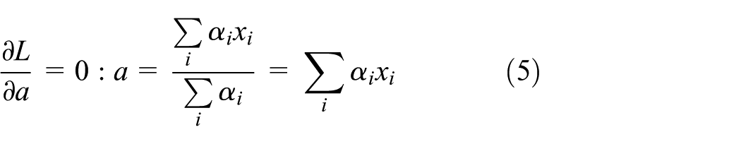
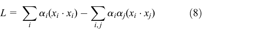
By substituting equations (4)–(6) into equation (3), equation (3) can be rewritten as follows
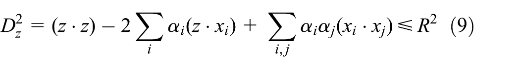
For determining whether a new point z is enclosed by the hypersphere, the distance between the center of the sphere and the point z must be calculated. The point z will not be rejected when the distance is smaller or equal to the radius
where
For giving a more flexible data description, the inner products


Any kernel functions have to satisfy Mercer’s theorem. 18 There are two kinds of kernel functions commonly used in practice: a polynomial kernel and a Gaussian kernel.
The polynomial kernel is as follows

where the free parameter
The Gaussian kernel is as follows

where s is the width parameter.
According to Lazzaretti et al., 19 the SVDD with the Gaussian kernel can generate an irregular-shaped hypersphere and have a better performance in data description. Therefore, the Gaussian kernel will be used in this article.
The parameters C and s are set to 1 and 5 in this article, and more detailed analysis is presented in section “Choice of SVDD parameters.” It should be noted that getting the optimal performance of proposed method is not the target of this study. The target of this study is obtaining a general performance to show the generality of our methods. Interested readers can refer to Wang et al. 20 They used genetic algorithm (GA) to search the optimal parameter combination of support vector regression (SVR) 21 and the results showed that their GA-SVR method was better than the mathematical regression model and artificial neural network (ANN).22–24
MCUSUM
According to Pignatiello and Runger,
6
CUSUM control charts
25
are often used instead of Shewhart control charts
26
when the detection of small shifts is of interest in univariate statistical process control. In other words, the CUSUM statistic has a better sensitivity for small shifts.
27
Based on an analogy of the univariate statistical process control, two multivariate extensions of the CUSUM control charts and the Shewhart control charts are generated naturally. They are Hotelling’s
Pignatiello and Runger proposed two statistics to construct different MCUSUM control charts, that is,
Here,

where x denotes the quality characteristics and

where
Approach for monitoring multivariate manufacturing process
D-MCUSUM control chart based on SVDD
In this study, a modified multivariate control chart based on SVDD is proposed to monitor the shift of manufacturing process, which is called
D-value and D chart
When the SVDD is trained by the collected normal data, the trained SVDD will generate a hypersphere characterized by “center” and “radius” that can represent the learned normal data space. After getting the trained SVDD, a

where t represents a n-dimensional moving window vector and the moving window vector consists of n
The
D-MCUSUM statistic
Although

where
The
A multivariate monitoring model based on the D-MCUSUM control chart
From what we have introduced above, an effective

In the offline learning module, a large number of in-control data will be collected automatically from various sensors embedded in manufacturing system because a learning model trained by data with a lot of noises must lead to an unsatisfactory result. Therefore, before inputting the collected in-control data to SVDD to train SVDD, some data preprocessing methods will be adopted to deal with the raw in-control data such as denoising and standardization. After preprocessing procedure, the distribution parameters of the in-control data will be estimated to calculate the
In the online monitoring module, some data preprocessing methods are also needed to deal with the raw data. After this, the
Generation of simulation data
To evaluate the performance of the
In the multivariate manufacturing process, there will usually be two or more correlated quality characteristics. In this study, a bivariate manufacturing process model is adopted to generate simulation data and it can be expressed in equation (18)

where
In this study, the mean shifts pattern is adopted in the out-of-control process. If an out-of-control pattern occurs in the process at time t, this can be expressed in equation (19)

where
Performance evaluation method
Moving window analysis method
For getting more real simulation results, a moving window analysis method29,30 is adopted in this article to input data to SVDD. There will be n observation points in the moving window each time. The dimension of the space that SVDD learned is determined by the moving window size. Every observation point is the

The application of the moving window analysis method.
The application of the moving window analysis method mainly consists of the following steps:
Step 1. Setting t (observation point) to n (window size).
Step 2. Taking the most recent n observation points,
Step 3. Making
In this article, we assume that the process is initially in control. This assumption can be considered more practical because in the real-world monitoring process an out-of-control signal often occurs after a period in which the process is in control, and the starting point of the out-of-control signal is usually unknown. 31
It should be pointed out that the moving window size will last a great effect on the proposed control chart. Therefore, it is essential to set an appropriate value of window size. For more details of this, it will be discussed in section “Choice of window size.”
ARL
ARL is a widely used performance criteria in the field of control charts. The ARL, in a sense, can indicate the sensitivity of control charts. 32 The ARL is defined as the average number of observations between the occurrence of out-of-control state and the alarm of out-of-control signal. In general, there are two kinds of ARLs, that is, in-control ARL and out-of-control ARL. The two kinds of ARLs are also related to the probabilities of two types of errors, that is, type I error and type II error. For in-control ARL, the larger the probability of type I error is, the shorter the in-control ARL will be. For out-of-control ARL, the larger the probability of type II error is, the longer the out-of-control ARL will be. There is usually a compromise between the two errors. Because when the type I error decreases, the type II error will increase. When the type II error decreases, however, the type I error will increase. An excellent control chart should minimize both the errors simultaneously. In other words, an excellent control chart should have the characteristics of longer in-control ARL and shorter out-of-control ARL.
It should be noted that an in-control ARL of 350 is adopted in this article to evaluate the performance of different control charts and the in-control ARL of 350 will make control charts have a relative small type I error. Specific steps of calculating the in-control ARL are summarized as follows:
Setting window number m to 1, t (observation point) to n (window size).
Feeding a window vector with n observation points (in-control data) to SVDD and calculating the
If the
Recording the value of the window number m as the run length of this trial.
For the calculation of out-of-control ARL, it is almost the same as in-control ARL. The only difference between them is the window vectors. For in-control ARL, every observation point of the window vectors is in-control data. For out-of-control ARL, however, initial several window vectors will include out-of-control data partially and every observation point of later window vectors is out-of-control data. The reason for this is that we assume that the process was initially in control. We can take an example to introduce this process. For instance, when window number
It should be noted that all the ARLs are computed from 10,000 independent simulation runs to get a stable result.
Control limit
In this study, a fixed control limit h is used to determine the state of the current process. When a
All the control limits are obtained based on in-control ARL of 350. The control limits will be tuned to make in-control ARL approximately equal to 350. All the control limits are computed from 10,000 independent simulations.
Simulation studies
Choice of window size
Before conducting simulation experiments, several key parameters should be determined. An appropriate window size will construct a better monitoring model. Therefore, a study will be conducted to select an appropriate widow size based on the ARL performances of different window sizes. Six kinds of different window sizes

where
In general, a large shift will have a better out-of-control ARL, that is, a smaller out-of-control ARL. In the study, we first take a shifts vector

Performance of different window sizes for a specific shifts pattern.
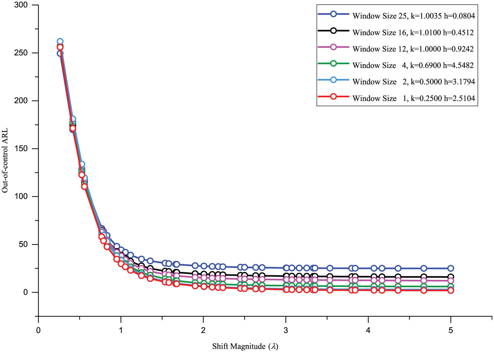
Performance of different window sizes.
As is shown in Figure 4, window size of 1 gets the best performance overall and this window size should be the best choice of the
Choice of SVDD parameters
The performance of SVDD is very dependent on the parameters C and s. Both will greatly affect the tightness of the data description boundary. To show this phenomenon, 200 two-dimensional banana data are generated. Figure 5 shows the different boundaries of the SVDD with different C and s. As shown in Figure 5, a small C or s will lead to a tighter boundary, which is equivalent to an overfitting phenomenon. However, a large C or s will generate a looser boundary. Therefore, the two parameters that become too small or too large can lead to an unsatisfactory data description boundary of SVDD due to overfitting or underfitting problem. Therefore, for avoiding the two problems, the parameters C and s are set to 1 and 5, respectively, to get a relative optimal detection performance in this article. After all, getting the optimal performance of the proposed method is not the target of this study. The target of this study is obtaining a general performance to show the generality of our methods.

Examples of SVDD with different values of C and s: (a) small values of C and s and (b) large values of C and s.
Simulation results and discussions
There may be various kinds of correlations between variables in the multivariate manufacturing process. Therefore, four different experiments are designed to testify the universality of the

where
Figure 6 shows the out-of-control ARL performance of the
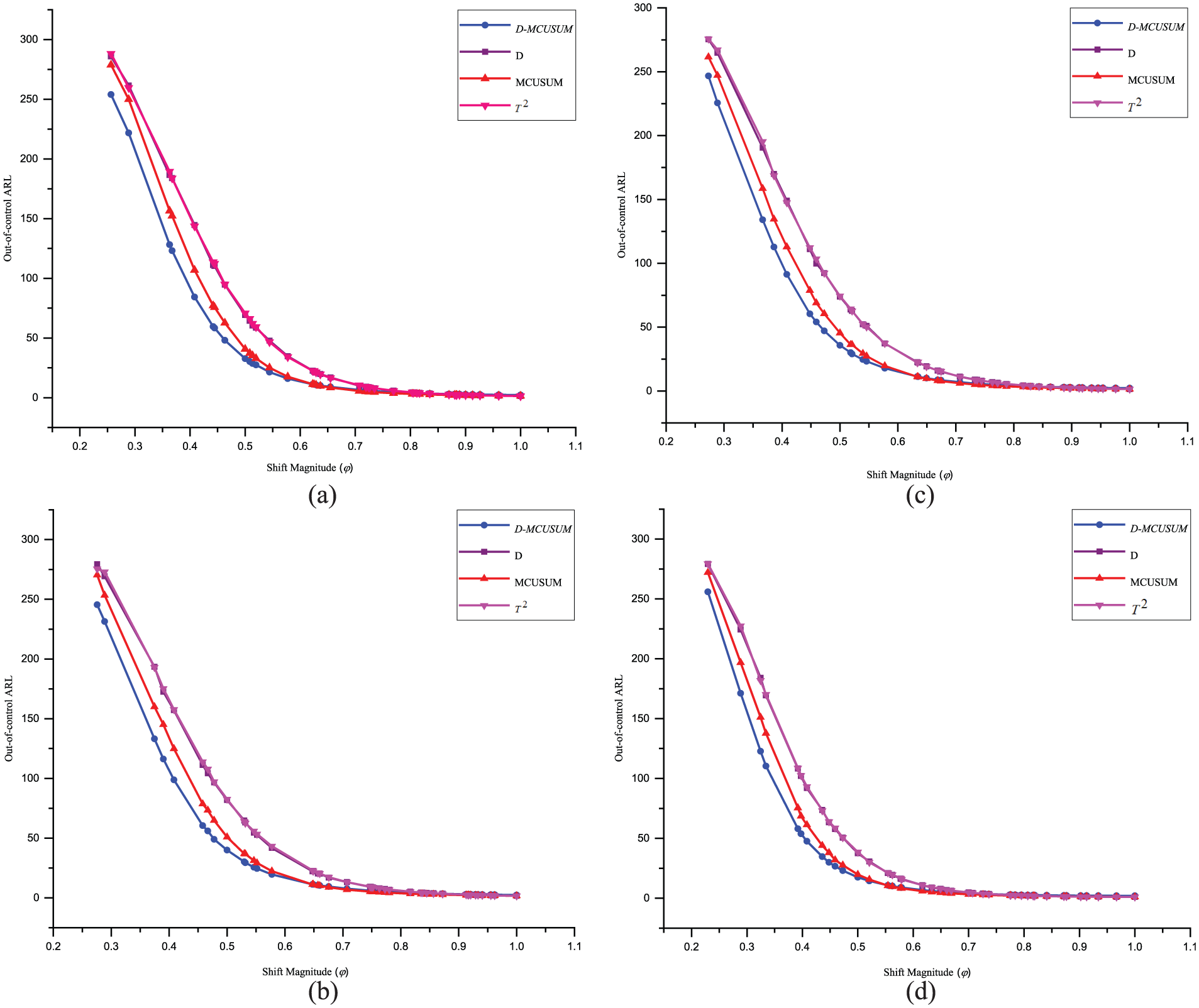
Comparisons of out-of-control ARL performance between the
The control limits and in-control ARLs of four control charts.

As is shown in Figure 6 and Table 2, the
Out-of-control ARL performance of the

The results also show that the
Illustrative example
In this section, a real industrial case derived from Alt 35 is provided to this study to demonstrate the applicability of the proposed control chart. Two quality characteristics of stiffness and bending strength from a lumber manufacturing plant are presented to represent a bivariate process. The in-control vector mean and covariance matrix are calculated based on the in-control data and they are given as follows

The in-control ARL of 350 is acceptable in this study.
We assume that a small shift magnitude of
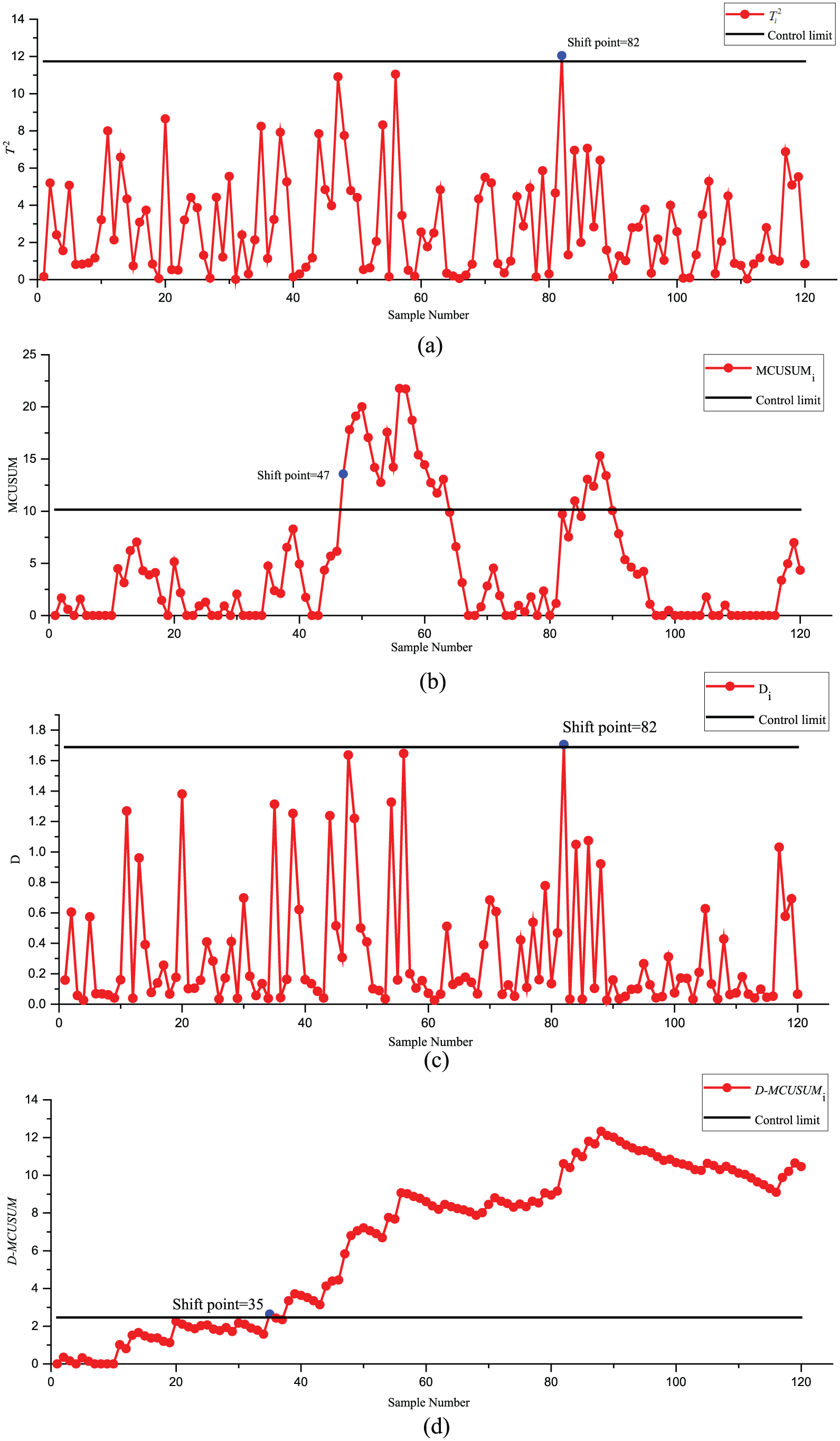
The
As is shown in Figure 7, the proposed control chart gives a faster out-of-control signal than other control charts at the 35th sample point. Moreover, the proposed control chart gives a continuous abnormal alarm after the 35th sample point. This shows the stability of the proposed control chart for detecting small shifts. This is a very important characteristic for practical applications and this characteristic is unavailable for other control charts. Therefore, this case gives a practical demonstration that the
Conclusion
In this article, we propose a modified MCUSUM control chart based on SVDD for detecting small mean shifts, which is named
To evaluate the performance of the
Besides these, the
From the above empirical analysis, all the results show that the
Some issues could be the topics of future research. As pointed out in section “SVDD,” the parameter optimization of SVDD still requires further investigation. Moreover, integrating the
Footnotes
Appendix
Data set for the illustrative example and other related statistics for different charts.

| Sample number | Stiffness | Bending strength | Standardization |
T 2 | MCUSUM | D | D-MCUSUM | |
|---|---|---|---|---|---|---|---|---|
| Stiffness | Bending strength | |||||||
| 1 | 266.41 | 467.62 | 0.14 | −0.22 | 0.1620 | 0.0000 | 0.1581 | 0.0000 |
| 2 | 258.19 | 446.37 | −0.68 | −2.15 | 5.1911 | 1.6911 | 0.6044 | 0.3544 |
| 3 | 279.53 | 474.82 | 1.45 | 0.44 | 2.4043 | 0.5954 | 0.0573 | 0.1616 |
| 4 | 276.36 | 482.02 | 1.14 | 1.09 | 1.5533 | 0.0000 | 0.0267 | 0.0000 |
| 5 | 281.27 | 467.04 | 1.63 | −0.27 | 5.0711 | 1.5711 | 0.5733 | 0.3233 |
| 6 | 257.82 | 470.10 | −0.72 | 0.01 | 0.8173 | 0.0000 | 0.0690 | 0.1423 |
| 7 | 273.05 | 471.56 | 0.80 | 0.14 | 0.8293 | 0.0000 | 0.0678 | 0.0000 |
| 8 | 274.34 | 477.54 | 0.93 | 0.69 | 0.8962 | 0.0000 | 0.0615 | 0.0000 |
| 9 | 269.96 | 464.84 | 0.50 | −0.47 | 1.1660 | 0.0000 | 0.0410 | 0.0000 |
| 10 | 277.46 | 466.86 | 1.25 | −0.29 | 3.2200 | 0.0000 | 0.1603 | 0.0000 |
| 11 | 273.88 | 452.23 | 0.89 | −1.62 | 7.9997 | 4.4997 | 1.2681 | 1.0181 |
| 12 | 279.45 | 477.60 | 1.44 | 0.69 | 2.1349 | 3.1346 | 0.0385 | 0.8066 |
| 13 | 290.54 | 484.79 | 2.55 | 1.34 | 6.5796 | 6.2142 | 0.9599 | 1.5165 |
| 14 | 265.95 | 452.31 | 0.10 | −1.61 | 4.3403 | 7.0546 | 0.3906 | 1.6571 |
| 15 | 272.15 | 470.49 | 0.71 | 0.04 | 0.7421 | 4.2966 | 0.0769 | 1.4840 |
| 16 | 266.72 | 486.53 | 0.17 | 1.50 | 3.0873 | 3.8839 | 0.1392 | 1.3732 |
| 17 | 261.11 | 450.77 | −0.39 | −1.75 | 3.7362 | 4.1201 | 0.2562 | 1.3794 |
| 18 | 270.47 | 467.15 | 0.55 | −0.26 | 0.8385 | 1.4586 | 0.0669 | 1.1963 |
| 19 | 263.88 | 471.09 | −0.11 | 0.10 | 0.0558 | 0.0000 | 0.1767 | 1.1230 |
| 20 | 283.00 | 461.42 | 1.80 | −0.78 | 8.6478 | 5.1478 | 1.3802 | 2.2532 |
| 21 | 271.20 | 477.45 | 0.62 | 0.68 | 0.5297 | 2.1775 | 0.1025 | 2.1057 |
| 22 | 258.84 | 462.74 | −0.62 | −0.66 | 0.5107 | 0.0000 | 0.1050 | 1.9607 |
| 23 | 247.25 | 456.29 | −1.77 | −1.25 | 3.2019 | 0.0000 | 0.1573 | 1.8680 |
| 24 | 246.27 | 449.24 | −1.87 | −1.89 | 4.4184 | 0.9184 | 0.4093 | 2.0273 |
| 25 | 280.66 | 469.87 | 1.57 | −0.01 | 3.8664 | 1.2848 | 0.2834 | 2.0607 |
| 26 | 265.09 | 480.11 | 0.01 | 0.92 | 1.3058 | 0.0000 | 0.0338 | 1.8445 |
| 27 | 264.13 | 471.83 | −0.09 | 0.17 | 0.0823 | 0.0000 | 0.1720 | 1.7665 |
| 28 | 275.15 | 460.49 | 1.02 | −0.86 | 4.4229 | 0.9229 | 0.4104 | 1.9269 |
| 29 | 273.64 | 481.73 | 0.86 | 1.07 | 1.2154 | 0.0000 | 0.0382 | 1.7151 |
| 30 | 287.27 | 491.45 | 2.23 | 1.95 | 5.5474 | 2.0474 | 0.6973 | 2.1624 |
| 31 | 264.28 | 468.54 | −0.07 | −0.13 | 0.0176 | 0.0000 | 0.1837 | 2.0961 |
| 32 | 280.37 | 478.39 | 1.54 | 0.76 | 2.4028 | 0.0000 | 0.0571 | 1.9032 |
| 33 | 270.52 | 473.38 | 0.55 | 0.31 | 0.3054 | 0.0000 | 0.1348 | 1.7880 |
| 34 | 268.39 | 459.73 | 0.34 | −0.93 | 2.1332 | 0.0000 | 0.0384 | 1.5764 |
| 35 | 293.61 | 486.75 | 2.86 | 1.52 | 8.2443 | 4.7443 | 1.3126 | 2.6390 |
| 36 | 267.64 | 462.66 | 0.26 | −0.67 | 1.1341 | 2.3784 | 0.0430 | 2.4320 |
| 37 | 281.41 | 474.37 | 1.64 | 0.40 | 3.2333 | 2.1117 | 0.1625 | 2.3445 |
| 38 | 292.77 | 492.33 | 2.78 | 2.03 | 7.9169 | 6.5286 | 1.2524 | 3.3469 |
| 39 | 285.01 | 493.06 | 2.00 | 2.10 | 5.2575 | 8.2861 | 0.6217 | 3.7186 |
| 40 | 268.52 | 470.96 | 0.35 | 0.09 | 0.1476 | 4.9337 | 0.1606 | 3.6292 |
| 41 | 270.48 | 473.06 | 0.55 | 0.28 | 0.3043 | 1.7380 | 0.1350 | 3.5141 |
| 42 | 271.76 | 470.38 | 0.68 | 0.03 | 0.6713 | 0.0000 | 0.0849 | 3.3490 |
| 43 | 267.83 | 462.67 | 0.28 | −0.67 | 1.1729 | 0.0000 | 0.0406 | 3.1396 |
| 44 | 288.76 | 498.73 | 2.38 | 2.61 | 7.8430 | 4.3430 | 1.2382 | 4.1278 |
| 45 | 286.79 | 481.66 | 2.18 | 1.06 | 4.8421 | 5.6852 | 0.5145 | 4.3923 |
| 46 | 262.73 | 451.07 | −0.23 | −1.72 | 3.9760 | 6.1611 | 0.3071 | 4.4494 |
| 47 | 276.78 | 450.63 | 1.18 | −1.76 | 10.9055 | 13.5667 | 1.6360 | 5.8354 |
| 48 | 291.97 | 481.70 | 2.70 | 1.06 | 7.7508 | 17.8174 | 1.2200 | 6.8055 |
| 49 | 248.73 | 446.39 | −1.63 | −2.15 | 4.7867 | 19.1042 | 0.5005 | 7.0560 |
| 50 | 257.81 | 447.88 | −0.72 | −2.01 | 4.4160 | 20.0202 | 0.4087 | 7.2147 |
| 51 | 261.77 | 462.09 | −0.32 | −0.72 | 0.5354 | 17.0556 | 0.1017 | 7.0664 |
| 52 | 272.76 | 476.71 | 0.78 | 0.61 | 0.6350 | 14.1906 | 0.0892 | 6.9056 |
| 53 | 253.62 | 470.16 | −1.14 | 0.01 | 2.0558 | 12.7464 | 0.0346 | 6.6902 |
| 54 | 284.20 | 463.72 | 1.92 | −0.57 | 8.3219 | 17.5683 | 1.3261 | 7.7664 |
| 55 | 268.68 | 471.18 | 0.37 | 0.11 | 0.1551 | 14.2234 | 0.1593 | 7.6757 |
| 56 | 298.20 | 490.64 | 3.32 | 1.88 | 11.0420 | 21.7654 | 1.6459 | 9.0716 |
| 57 | 275.25 | 463.14 | 1.02 | −0.62 | 3.4479 | 21.7133 | 0.2001 | 9.0217 |
| 58 | 269.88 | 477.75 | 0.49 | 0.70 | 0.5035 | 18.7168 | 0.1060 | 8.8777 |
| 59 | 269.25 | 473.08 | 0.43 | 0.28 | 0.1819 | 15.3987 | 0.1548 | 8.7824 |
| 60 | 265.64 | 456.36 | 0.06 | −1.24 | 2.5580 | 14.4567 | 0.0715 | 8.6040 |
| 61 | 277.88 | 475.60 | 1.29 | 0.51 | 1.7688 | 12.7256 | 0.0264 | 8.3804 |
| 62 | 280.80 | 479.63 | 1.58 | 0.88 | 2.5042 | 11.7298 | 0.0662 | 8.1966 |
| 63 | 281.23 | 467.67 | 1.62 | −0.21 | 4.8293 | 13.0591 | 0.5113 | 8.4579 |
| 64 | 268.26 | 467.90 | 0.33 | −0.19 | 0.3398 | 9.8989 | 0.1295 | 8.3374 |
| 65 | 266.91 | 467.73 | 0.19 | −0.21 | 0.1975 | 6.5964 | 0.1522 | 8.2396 |
| 66 | 266.92 | 470.10 | 0.19 | 0.01 | 0.0546 | 3.1510 | 0.1769 | 8.1665 |
| 67 | 260.34 | 465.33 | −0.47 | −0.42 | 0.2498 | 0.0000 | 0.1436 | 8.0601 |
| 68 | 256.10 | 462.45 | −0.89 | −0.69 | 0.8289 | 0.0000 | 0.0679 | 7.8780 |
| 69 | 285.51 | 486.72 | 2.05 | 1.52 | 4.3370 | 0.8370 | 0.3898 | 8.0178 |
| 70 | 284.07 | 494.59 | 1.91 | 2.24 | 5.4967 | 2.8337 | 0.6841 | 8.4519 |
| 71 | 286.89 | 490.12 | 2.19 | 1.83 | 5.2051 | 4.5388 | 0.6080 | 8.8099 |
| 72 | 256.51 | 461.04 | −0.85 | −0.81 | 0.8661 | 1.9049 | 0.0643 | 8.6242 |
| 73 | 267.03 | 466.40 | 0.20 | −0.33 | 0.3565 | 0.0000 | 0.1270 | 8.5011 |
| 74 | 274.90 | 475.39 | 0.99 | 0.49 | 0.9978 | 0.0000 | 0.0528 | 8.3039 |
| 75 | 268.77 | 454.18 | 0.38 | −1.44 | 4.4695 | 0.9695 | 0.4217 | 8.4756 |
| 76 | 281.89 | 482.55 | 1.69 | 1.14 | 2.8790 | 0.3484 | 0.1093 | 8.3348 |
| 77 | 276.46 | 460.82 | 1.15 | −0.83 | 4.9331 | 1.7815 | 0.5377 | 8.6226 |
| 78 | 265.92 | 473.88 | 0.09 | 0.35 | 0.1470 | 0.0000 | 0.1607 | 8.5333 |
| 79 | 260.96 | 446.33 | −0.40 | −2.15 | 5.8578 | 2.3578 | 0.7781 | 9.0614 |
| 80 | 270.24 | 471.92 | 0.52 | 0.17 | 0.3046 | 0.0000 | 0.1349 | 8.9463 |
| 81 | 283.24 | 471.89 | 1.82 | 0.17 | 4.6549 | 1.1549 | 0.4674 | 9.1637 |
| 82 | 299.38 | 488.46 | 3.44 | 1.68 | 12.0492 | 9.7041 | 1.7047 | 10.6184 |
| 83 | 268.12 | 462.29 | 0.31 | −0.70 | 1.3299 | 7.5340 | 0.0328 | 10.4011 |
| 84 | 283.66 | 465.91 | 1.87 | −0.37 | 6.9533 | 10.9872 | 1.0485 | 11.1997 |
| 85 | 278.92 | 481.35 | 1.39 | 1.03 | 1.9986 | 9.4859 | 0.0322 | 10.9819 |
| 86 | 287.58 | 497.24 | 2.26 | 2.48 | 7.0645 | 13.0504 | 1.0740 | 11.8058 |
| 87 | 278.79 | 487.61 | 1.38 | 1.60 | 2.8363 | 12.3867 | 0.1036 | 11.6595 |
| 88 | 287.43 | 474.42 | 2.24 | 0.40 | 6.4216 | 15.3083 | 0.9212 | 12.3306 |
| 89 | 265.81 | 459.46 | 0.08 | −0.96 | 1.5918 | 13.4001 | 0.0262 | 12.1068 |
| 90 | 268.80 | 471.66 | 0.38 | 0.15 | 0.1536 | 10.0537 | 0.1596 | 12.0164 |
| 91 | 261.84 | 458.38 | −0.32 | −1.06 | 1.2752 | 7.8289 | 0.0352 | 11.8016 |
| 92 | 255.04 | 462.10 | −1.00 | −0.72 | 1.0147 | 5.3437 | 0.0514 | 11.6030 |
| 93 | 268.24 | 457.72 | 0.32 | −1.12 | 2.7883 | 4.6319 | 0.0975 | 11.4506 |
| 94 | 278.24 | 487.83 | 1.32 | 1.62 | 2.8195 | 3.9514 | 0.1015 | 11.3020 |
| 95 | 247.59 | 450.88 | −1.74 | −1.74 | 3.7825 | 4.2339 | 0.2657 | 11.3177 |
| 96 | 264.06 | 464.23 | −0.09 | −0.52 | 0.3516 | 1.0855 | 0.1277 | 11.1955 |
| 97 | 279.57 | 481.85 | 1.46 | 1.08 | 2.1882 | 0.0000 | 0.0416 | 10.9871 |
| 98 | 263.19 | 477.63 | −0.18 | 0.69 | 1.0394 | 0.0000 | 0.0496 | 10.7866 |
| 99 | 275.46 | 491.90 | 1.05 | 1.99 | 3.9963 | 0.4963 | 0.3116 | 10.8482 |
| 100 | 269.37 | 459.28 | 0.44 | −0.97 | 2.5812 | 0.0000 | 0.0739 | 10.6720 |
| 101 | 263.06 | 470.61 | −0.19 | 0.06 | 0.0833 | 0.0000 | 0.1718 | 10.5939 |
| 102 | 265.71 | 473.14 | 0.07 | 0.29 | 0.0973 | 0.0000 | 0.1693 | 10.5132 |
| 103 | 270.19 | 464.36 | 0.52 | −0.51 | 1.3299 | 0.0000 | 0.0328 | 10.2960 |
| 104 | 283.68 | 482.88 | 1.87 | 1.17 | 3.4936 | 0.0000 | 0.2086 | 10.2545 |
| 105 | 287.51 | 480.78 | 2.25 | 0.98 | 5.2793 | 1.7793 | 0.6273 | 10.6319 |
| 106 | 260.64 | 464.00 | −0.44 | −0.55 | 0.3162 | 0.0000 | 0.1331 | 10.5150 |
| 107 | 261.01 | 455.26 | −0.40 | −1.34 | 2.0525 | 0.0000 | 0.0345 | 10.2995 |
| 108 | 281.30 | 468.83 | 1.63 | −0.11 | 4.4953 | 0.9953 | 0.4280 | 10.4774 |
| 109 | 264.63 | 477.98 | −0.04 | 0.73 | 0.8753 | 0.0000 | 0.0634 | 10.2908 |
| 110 | 273.74 | 476.14 | 0.87 | 0.56 | 0.7660 | 0.0000 | 0.0743 | 10.1152 |
| 111 | 264.22 | 467.91 | −0.08 | −0.19 | 0.0381 | 0.0000 | 0.1799 | 10.0451 |
| 112 | 273.26 | 479.01 | 0.83 | 0.82 | 0.8459 | 0.0000 | 0.0662 | 9.8613 |
| 113 | 275.82 | 476.98 | 1.08 | 0.63 | 1.1708 | 0.0000 | 0.0407 | 9.6520 |
| 114 | 281.62 | 482.59 | 1.66 | 1.14 | 2.7950 | 0.0000 | 0.0984 | 9.5004 |
| 115 | 265.21 | 479.35 | 0.02 | 0.85 | 1.0967 | 0.0000 | 0.0455 | 9.2959 |
| 116 | 264.82 | 461.09 | −0.02 | −0.81 | 0.9987 | 0.0000 | 0.0527 | 9.0986 |
| 117 | 290.18 | 493.06 | 2.52 | 2.10 | 6.8761 | 3.3761 | 1.0306 | 9.8792 |
| 118 | 274.27 | 458.02 | 0.93 | −1.09 | 5.0849 | 4.9610 | 0.5769 | 10.2060 |
| 119 | 279.12 | 462.78 | 1.41 | −0.66 | 5.5282 | 6.9893 | 0.6923 | 10.6483 |
| 120 | 274.07 | 474.49 | 0.91 | 0.41 | 0.8505 | 4.3397 | 0.0658 | 10.4641 |
Handling Editor: Kang Cheung Chan
Declaration of conflicting interests
The author(s) declared no potential conflicts of interest with respect to the research, authorship, and/or publication of this article.
Funding
The author(s) disclosed receipt of the following financial support for the research, authorship, and/or publication of this article: This project is supported by National Natural Science Foundation of China (grant no. 71401098).