
Abstract
The direct tuning of controller parameters, which is based on data-driven control, has been attracting considerable attention because of the ease of its control system design. In practical use, it is important to consider the stability of the closed-loop system and model matching with few design parameters. In this study, we propose a direct tuning method based on a fictitious reference signal that considers the bounded-input bounded-output (BIBO) and model matching without repeating experiments. The proposed method includes two steps. In the first step, the BIBO stability is satisfied. The pole information is lost in the cost function of the conventional method using a fictitious reference signal. Then, we derive a new cost function that can prevent the loss of the pole information. This provides controller parameters that can stabilize the closed-loop system. The model matching between the reference model and the closed-loop system is considered in the second step. When model matching is achieved, the characteristics of the reference model almost match those of the closed-loop system, including the gain and phase margins. The parameters of the reference model are automatically tuned to realize model matching. Using the two-step method, we can obtain parameters considering BIBO stability and the model matching. In addition, there are no design parameters apart from the dealing noise. Two simulations and an experiment were performed on a system with dead time to verify the effectiveness of the proposed two-step method. The results showed that the proposed method provides BIBO stability and model-matched control parameters from the measured data through a one-time experiment without trial and error.
Keywords
Introduction
In many industries, the number of controllers increases with the rapid increase in the number of electronic devices. Trial-and-error tuning of controller parameters is usually performed to obtain the desired control performance. The main problem associated with this tuning process is that the development period increases. Further, this is dependent on individual skills. Model-based control can also be applied, but more than 90% of the controllers used in industry are proportional–integral–derivative (PID) control. 1 Intuitive understanding and low computational cost are important factors. Therefore, studies on model-free control and data-driven control (DDC), wherein controller parameters are directly tuned using the input/output data of a controlled object, are attracting attention.2–21 Model-free control is effective when applied to time-varying systems because optimal parameters can be obtained via online calculations. However, some difficulties are associated with its application to mass products from the viewpoint of stability and CPU performance. Regardless, DDC, such as virtual reference feedback tuning (VRFT) 3 and fictitious reference iterative tuning (FRIT),4–6 can be used to obtain optimal controller parameters from the one-shot input/output data of the control object offline for the linear time invariant (LTI) systems. The development man-hours can be reduced because the controller parameters are obtained from data without repeating experiments or trial-and-error tuning. The direct tuning method based on DDC has been adopted in industries and is currently applied to industrial systems.22–26
One of the problems associated with the DDC design methods is that the closed-loop system is not always stable when the obtained control parameters are used.27–29 For example, a closed-loop system can be destabilized using the control parameters obtained with a DDC design method that uses a fictitious reference signal30,31 such as FRIT. This is likely to occur when an inappropriate reference model is given. This can be mitigated by applying a prefilter to the input and output data; subsequently, a power spectral density (PSD) function is required for designing the prefilter. 3 It is not difficult to estimate the PSD function of the initial input signals because VRFT uses the input/output data from open-loop experiments with random signals as its input signals; thus, a prefilter can be designed. However, although the PSD function is suitable for analyzing stationary random signals, it is not suitable for analyzing transient time-series signals. Therefore, it is difficult to estimate the PSD function using the input/output data obtained from a closed-loop experiment. 32 In addition, although the aforementioned problem can be avoided by tuning the reference model, this is a trial-and-error process. Thus, the control parameters cannot be obtained automatically in all the tuning processes.
Several methods have been proposed that consider DDC stability. Extended FRIT (E-FRIT) has been proposed,22,23 in which the weight of the control input is included in the objective function. This method can effectively suppress any destabilization because of excessive fluctuations in the control input. However, this is not an essential improvement with respect to the general problem of closed-loop system destabilization. DDC considering the stability method28,29 has been proposed based on the model validation knowledge in the time domain. However, (i) it takes time to calculate the singular values of the Toeplitz matrix and (ii) the stability must be confirmed each time optimization is performed. A VRFT process that considers robust stability has been proposed for a control structure based on the IMC; 25 however, it cannot be applied to a PID controller. The DDC design methods are for model matching. In case of unfalsified control, a previous study 33 showed that the instability of a closed-loop system cannot be detected because unstable poles are canceled when calculating the transfer function, namely the sensitivity function, the input of which is the fictitious reference signal and the output of which is the error between the fictitious reference signal and the controlled-object output. Then, a new objective function was proposed to detect the instability of the closed-loop system.33–35 Unlike the two aforementioned methods,22,23,25,28,29 the method proposed in another study 33 sets an objective function that minimizes the error between the target value and the controlled-object output and is applied to unfalsified control, which switches online between multiple controllers designed in advance. In other words, it is not applied to a method for obtaining optimal control parameters based on model matching such as FRIT.
In this study, we propose a direct tuning method for the feedback controller parameters based on the fictitious reference signal considering the bounded-input bounded-output (BIBO) stability and model matching without repeating experiments. The proposed method comprises two steps. In the first step, BIBO stability is satisfied. Stability cannot be detected with respect to the cost function of the FRIT, which is a conventional DDC method that uses fictitious reference signals because of the loss of pole information. To address this problem, we derive a new FRIT objective function that retains the pole information using a transfer function (complementary sensitivity function) identified in the time domain, the input and output of which are the fictitious reference signal, which is a function of the control parameters, and the controlled-object output, respectively. Herein, FRIT that enables the detection of instability in a closed-loop system is referred to as instability-detecting FRIT (ID-FRIT). Therefore, parameters that stabilize the closed-loop system are obtained because the pole information is retained in the objective function of the ID-FRIT. In the second step, we aim to obtain the parameters for model matching. When model matching is realized, the characteristics including gain and phase margins between user-defined reference model and closed-loop system are almost identical. The controller parameters and the dead time that minimize the objective function are obtained by including the dead time as the tuning parameter in the objective functions of the ID-FRIT. Further, the parameters related to responsiveness are optimized by comparing the obtained reference-model dead time and the identified controlled-object dead time from the input/output data measured in advance, thereby ensuring that the reference-model and identified dead times match. In this way, the reference-model parameters that enable model matching can be obtained. Thus, we can obtain parameters for model matching by automatically tuning the reference-model parameters. In the conventional method, a designer is used to tune the reference-model parameters. The optimization of the reference-model parameters requires the usage of ID-FRIT to detect destabilization. The effectiveness of the proposed method is verified via two simulations and an experiment.
This paper is arranged as follows. First, we explain the problem setting and the standard FRIT method as well as why destabilizing parameters are obtained, which is the problem associated with the conventional FRIT method. Second, we propose FRIT that considers stability. Third, we verify the proposed control method via simulation for two types of systems. Fourth, experimental validation is conducted. The controlled objects are systems with dead time. Dead time is worth considering because it is associated with many industrial systems, as represented by delays in material transport and signal transmission. For the controlled objects with dead time, the optimum control parameters of the conventional and proposed methods are obtained. By applying each set of obtained parameters to the closed-loop system, (i) ID-FRIT leads to BIBO stable control parameters, whereas standard FRIT leads to an unstable closed-loop system. (ii) Further, the parameters that realize model matching are obtained in the proposed method. Finally, the conclusions of this paper are discussed.
Preliminary
Here, we explain the problem statement and the standard FRIT4–6 proposed in previous studies along with its problems.
Problem statement
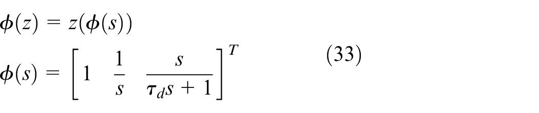
We consider a general feedback control system with a reference model, as shown in Figure 1. r, u, y, and yr indicate the target value (reference input), control input (manipulated variable), controlled-object output (controlled variable), and reference model output, respectively. P is the controlled object, which is an unknown LTI and SISO (single-input single-output) system. C(θ) is a linear fixed-order controller parameterized using the tunable parameter vector θ. For instance, C(θ) in the z-domain is described as
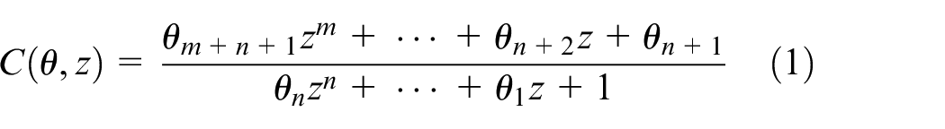
where
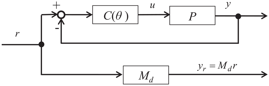
Closed system with tunable parameters.
Conventional standard FRIT
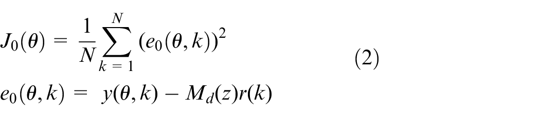
FRIT4–6 is a technique for automatically tuning the controller parameters of a closed-loop system from the controlled-object input/output data. Herein, we describe the FRIT procedures. First, the time-series input/output data {u0(k) and y0(k); k=1, 2, …, N} are obtained by conducting a closed-loop experiment using controller parameters that stabilize the system. Next, using the acquired initial input/output time-series data and the inverse of controller, the fictitious reference signal 30,31 can be calculated as

where
is minimized to obtain the optimal controller parameters.
Problems with conventional standard FRIT
The instability of a closed-loop system cannot be detected via FRIT. This assertion is based on a method proposed by a previous study, 33 which showed that the sensitivity functions with respect to the errors (the differences between the target values and controlled-object responses) and the fictitious reference signals cannot detect unstable poles because the sensitivity function does not contain pole information. Herein, we focus on the transfer function for the tracking error and the fictitious reference signal that we consider in FRIT. Based on the z-transform of the tracking error of equation (2), we obtain
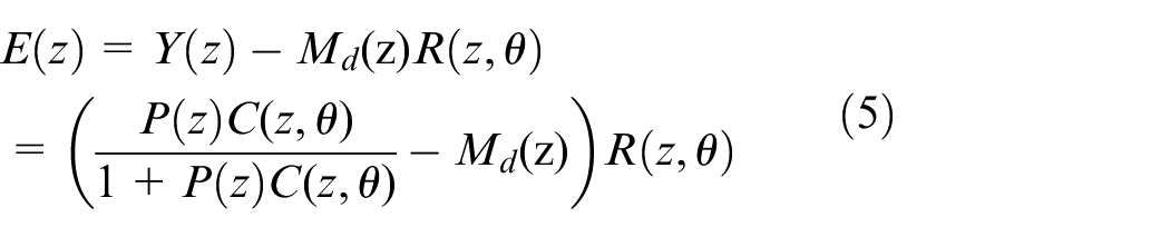
based on which unstable poles can be detected because equation (5) retains the information about the poles of the closed-loop system.
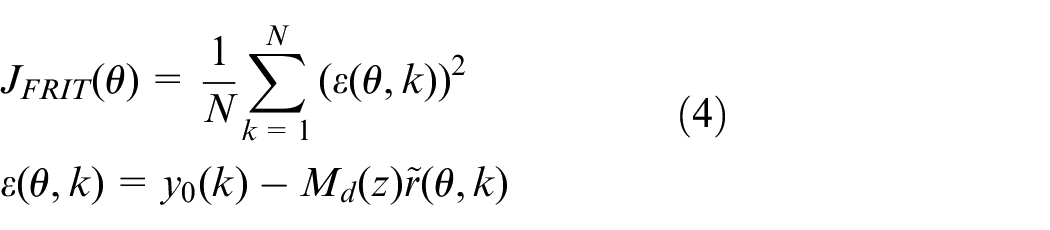
Next, we consider the tracking error handled by the FRIT of equation (4). The relation between the fictitious reference signal
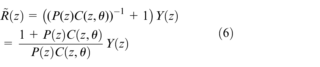
where Y(z) = P(z)U(z) was considered. From equations (3), (4), and (6), the relation between the error handled by the FRIT and the fictitious reference signal can be given as follows:
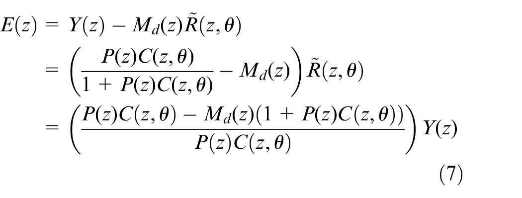
This equation shows that no pole can be obtained because of the pole-zero cancelation. Thus, the closed-loop system may become unstable when the control parameter that minimizes the objective function shown in equation (4) is obtained.
FRIT considering stability
In this section, we explain (i) the derivation of the FRIT objective functions considering the detection of destabilization to ensure that the closed-loop system exhibits BIBO stability and (ii) a method optimizing the reference-model parameters for model matching. Thus, if model matching is realized, the gain and phase margins of the reference model and the closed-loop stability are almost identical. In other words, the gain and phase margins are indirectly considered through the realization of model matching.
Derivation of the FRIT cost function considering destabilization detection
We derive the cost function by considering destabilization detection to obtain the parameters based on which closed-loop BIBO stability can be achieved. Stability can be evaluated by applying the target value r to the complementary sensitivity function for the controller C(z, θ) and calculating its output y*. The relation between the target value and the output of the closed-loop system is
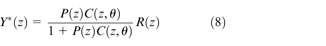
Because P(z) is unknown, the complementary sensitivity function of the controller C(z, θ) to be tuned can be written as
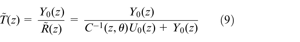
using the controlled-object input/output data acquired in advance. When the complementary sensitivity function in the frequency domain is identified as shown in equation (9), we require (i) the application of the parametric identification method using an ARX model or similar models and (ii) information about the order of the controlled object.
Here, the complementary sensitivity function is identified in the time domain to automatically tune the control parameters without using prior information such as the model structure and order. In the time domain, the relation between the fictitious reference signal and the controlled-object output is

where the asterisk indicates convolution and

where

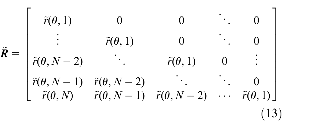

Here,
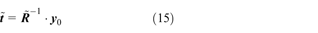
Next, the output when the target value is applied to the complementary sensitivity function is

which is calculated by considering

where

As described above, the output y* contains pole information because y* is calculated using

The standard FRIT tunes the fictitious reference signal, which is a function of the controller parameters, to match the measured controlled-object output y0. The proposed method tunes the controlled-object output, which is a function of the control parameters, to ensure that the controlled-object output y*, which is the predicted value, matches the reference-model output. The standard FRIT obtains the controller parameters to match the controlled-object output measured in advance via an experiment, whereas the proposed method obtains the control parameters to match the reference model output.
As described above, the parameter tuning algorithm is as follows. The part after Step 1-2 differs from the conventional standard FRIT and is the part in which stability is considered.
Step 0 Measuring the input/output data of the controlled object
The input/output data u0, y0 of the closed-loop system are measured using the initial values of the controller parameters. How to deal with noise is discussed in “Dealing with noise”.
Step 1-1 Calculating the fictitious reference signal
The fictitious reference signal is calculated from the acquired input/output data obtained using equation (3).
Step 1-2 Computing complementary sensitivity functions in the time domain
The complementary sensitivities are obtained from equation (15) using the calculated fictitious reference signal and the controlled-object outputs acquired in Step 0.
Step 1-3 Calculating the outputs of complementary sensitivity functions
The output y* of the complementary sensitivity function when the target value is applied is obtained from equation (17).
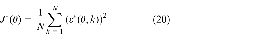
Step 1-4 Optimal parameters calculated by minimizing the objective function J*
The controller parameter θ that minimizes the objective function (20) is obtained using an optimization technique.
Poles are not directly calculated in this algorithm. Instead, we use the output y* calculated using equation (17) because the complementary sensitivity function
Dealing with noise
In an actual environment, the input/output data contain observation noise. In the open-loop test, the output is

where n is the white noise. In case of the closed-loop test, the measured input and output are
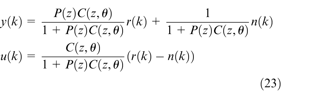
The r component of y is the low-pass characteristic of the complementary sensitivity function, which exhibits attenuation in the high-frequency range. Additionally, the n component of y is the high-pass characteristic of the sensitivity function, and it is coordinated in the high-frequency range. Therefore, for y, the signal-to-noise ratio (S/N) in the high-frequency range becomes worse. Further, if r and n are assumed to be a step signal and white noise, respectively, the S/N at high frequencies also deteriorates for u. 40
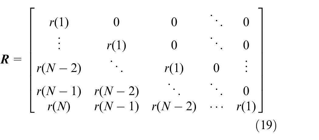
As shown in equation (24), the total variation denoising is used to eliminate noise from the time-series data of the control target output and control input with added noise. This method is based on the regression problem and noisy data are restored to denoised data. In image processing, the L1 norm is commonly used as the regularization term; however, in case of time-series data, the L2 norm is adopted as the regularization term because the L1 norm tends to be a staircase signal. The denoising equation is described as
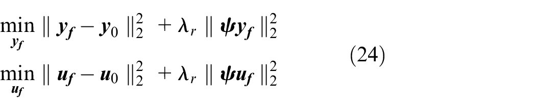
where
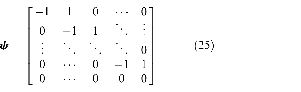
Here,
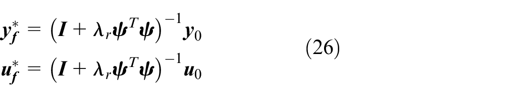
where I is the identity matrix with size N × N.
We summarize the aforementioned equations as Step 0 in the algorithm, which includes the denoising process as follows:
Step 0-1 Measuring the input/output data of the controlled object
The raw input/output time-series data is obtained via experiment.
Step 0-2 Performing the denoising process
The denoised input/output time-series data measured in Step 0-1 is obtained using equation (26).
This algorithm provides the denoised input/output data, which are used in the control parameters optimization.
Method for optimizing the reference model
Conventionally, the reference-model parameters are tuned by the designer in a trial-and-error manner because performance degradation can be observed when using an inappropriate reference model. 41 Herein, the characteristics, including the gain and phase margins of the system and those of the reference model, are considered to be almost identical when model matching is realized. In other words, the gain and phase margins can be indirectly considered before implementing the controller by realizing model matching. The details are described in “Discussion about system 1”. Herein, we propose a technique to optimize the reference-model parameters for model matching using dead times. First, dead times are identified from the input/output data acquired in Step 0 of the algorithm. Next, a variable reference model in which dead time is considered as a tuning parameter is introduced as follows:
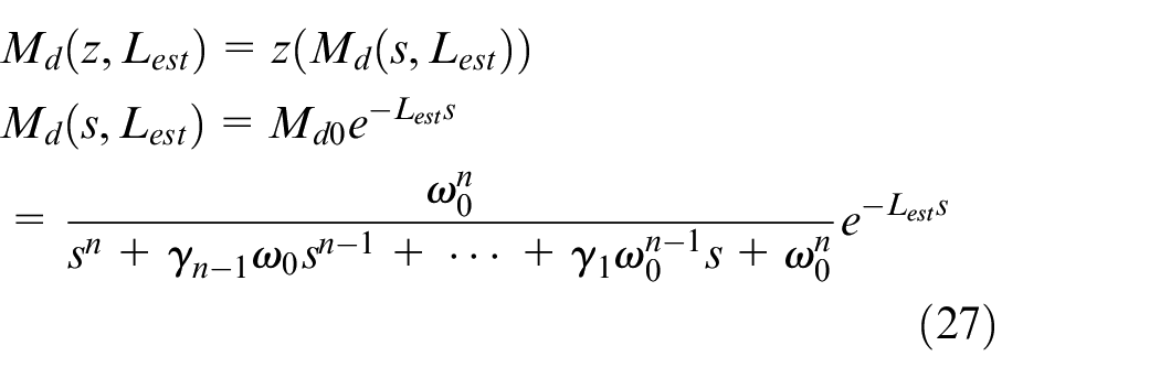
Here, s is the Laplacian operator, Lest is a tuning parameter related to the dead time, ω0 is a design parameter related to responsiveness, γ is a design parameter for determining the characteristics of the reference model, and z() is an operator for converting from the continuous time domain to the discrete time domain. The controller parameters and dead time can be estimated by replacing the reference model of the objective function in equation (20) with a variable reference model and minimizing the objective function.
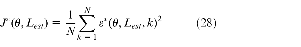

At this time, the controller parameters and reference-model dead time that minimize the objective function of equation (28) are obtained via optimization calculation. If the obtained reference-model dead time coincides with the identified controlled-object dead time, then the parameters for which model matching can be realized using a controller of the specified order are found. However, if the reference-model dead time does not coincide with the identified one, then either the order of the controller must be increased or the target reference response must be decelerated. Thus, the appropriate reference-model parameters are tuned automatically. The algorithm is as follows.
Step 2-1 Dead times are identified from the input/output data acquired in advance.
Step 2-2 Controller parameters and reference-model dead time are estimated that minimize the FRIT objective functions considering the detection of destabilization (i.e. ID-FRIT proposed in Step 1), including variable reference models, as shown in equation (28).
Step 2-3 Tuning of parameters related to the responsiveness of the reference model
(a) Estimated reference model dead time > identified dead time: (a-1) or (a-2)
(a-1) Increase the reference-model responsiveness parameter as τM←τM+ΔτM
(a-2) Increase the order of the controller.Else: Return to Step 2-2.
(b) Estimated reference model dead time <= identified dead time: End
Note that ID-FRIT needs to be used in this algorithm. In the case where conventional FRIT is used, we may not obtain an appropriate responsiveness parameter in Step 2 because the closed-loop system may become unstable when the objective function based on conventional FRIT, that is,
As shown above, the proposed method can tune the controller parameters in consideration of the BIBO stability and model matching without repeating the experiment from the one-shot input/output data of the controlled object. In addition, no design parameters except those dealing with noise are necessary.
Simulation validation
The proposed method was verified via two numerical simulations. One numerical simulation is a process system without and with noise, whereas the other is a spring-mass system with noise. We describe the formulation of a reference model and the controller used in this section. Similar to that in previous studies,5,8,42 the reference model is a second-order binomial-coefficient standard form in which no overshoot occurs, that is,
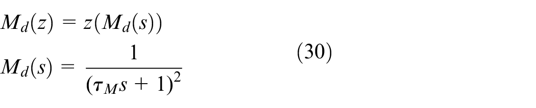
where τM is a parameter related to the responsiveness of the system. The controller C(z) is the PID controller and can be given as

With

where Kp, Ki, and Kd are the proportional, integral, and derivative gains, respectively. In this study, because a PID controller is used, Step 2-3(a-1) of increasing the responsiveness parameter of the reference model is performed instead of changing the order of the controller. The controller and controlled object are discretized by a zero-order hold.
Application to system1: Process system
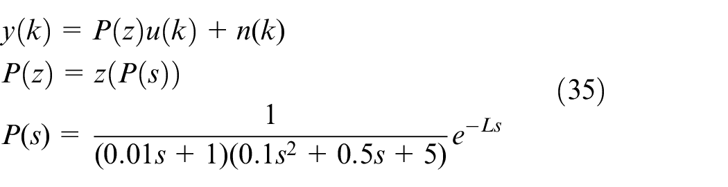
The controlled object P is an actual process system8,43,44 often considered to be a numerical example or benchmarking problem of DDC. Moreover, the dead time L is added to the system. 5 Many industrial systems involve dead times, as indicated by the delays in the transport of materials and the transmission of signals, making it considerably difficult to obtain stable parameters. Therefore, we show the effectiveness of the proposed method for a system with added dead time. The controlled object is
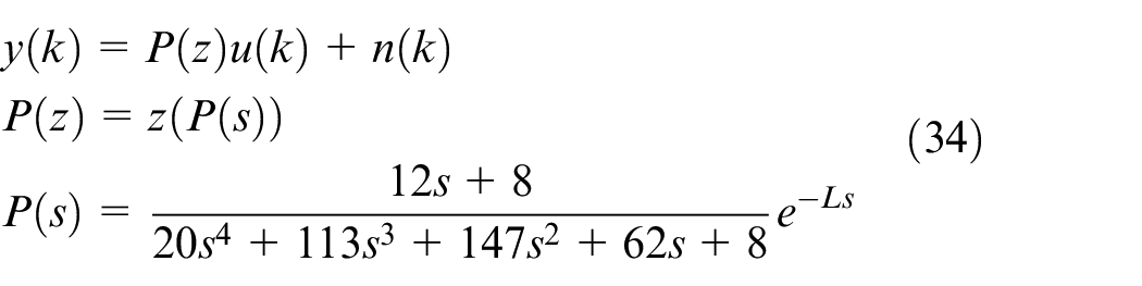
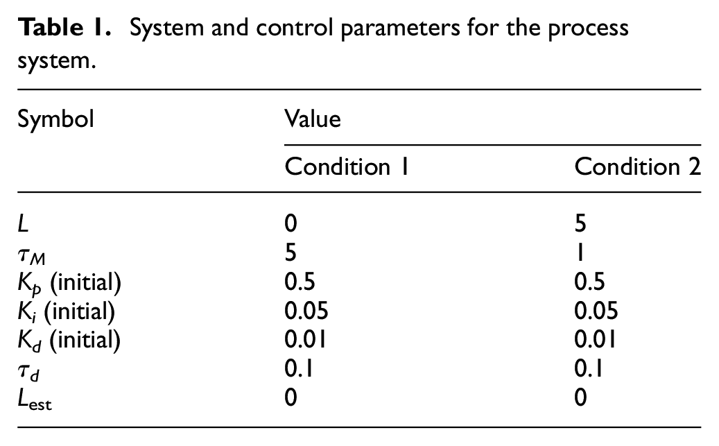
where L is the dead time and n is the white noise. The sampling period is 100 ms. The parameter sets are presented in Table 1, and the simulation is performed for conditions 1 and 2. In condition 1, by assuming that model matching is possible, the controlled object has no dead time and the responsiveness parameter of the reference model is set to a large value. In condition 2, by assuming that model matching cannot be performed, the controlled object has a dead time and the responsiveness parameter of the reference model is set to a small value. The dead time values are the same as those in the literature,4,5 and the conventional and proposed methods are compared in simulations under these two conditions.
System and control parameters for the process system.
Simulation results
[Case 1: Ideal condition]
The proposed method is verified by considering the ideal condition; thus, the variance of white noise shown in equation (34) is zero.
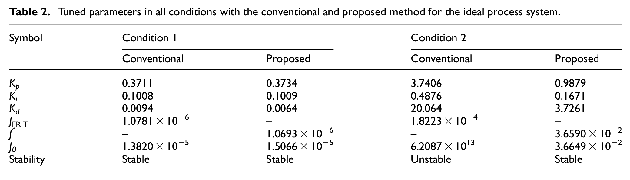
First, we confirm the effectiveness of ID-FRIT using Step 1 of the algorithm. Figure 2 shows the time history when the initial parameter values are used. Figure 3 shows the time history of the input/output data with the conventional FRIT and the proposed method when the step input under condition 2 is applied to the closed-loop system. Figure 4 shows the values of the objective function for a particular number of PSO iterations. Although Figure 4 shows that the objective functions of the standard FRIT converge, the output data of the standard FRIT shown in Figure 3 are divergent. In contrast, in the proposed method, the controller parameters that stabilize the closed-loop system are obtained even when model matching cannot be realized. The simulation results are presented in Table 2, which is used in the discussion section.
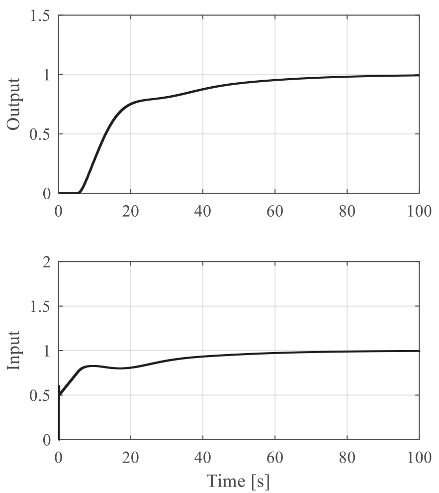
Input and output time series data with the initial PID gain for the ideal process. Dead time is 5.0 s.
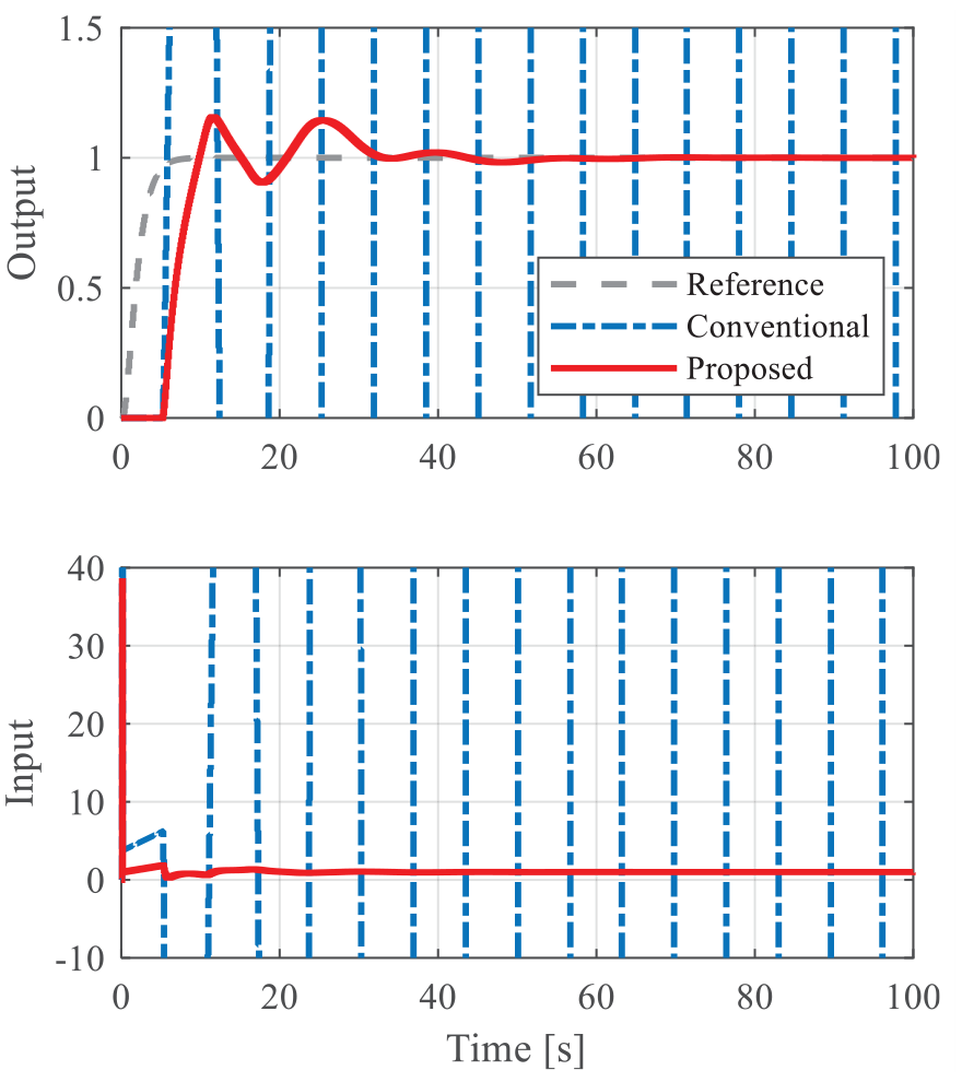
Input and output time series data with the conventional and proposed methods under condition 2 for an ideal process.
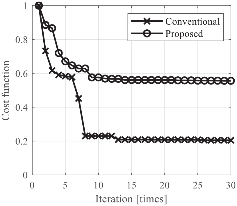
Relationship between the normalized cost function and optimization iterations.
Tuned parameters in all conditions with the conventional and proposed method for the ideal process system.
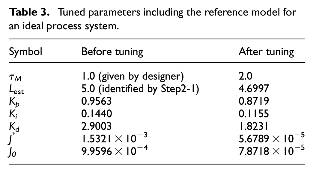
Next, we confirm the effectiveness of the reference-model optimization method by applying Step 2 of the algorithm. The reference model with a tunable parameter Lest, which is added to equation (30), is used as described in the subsection titled “Method for optimizing the reference model.” The controlled-object dead time is 5.0 s from Table 1. Figure 5 shows the time histories of the closed-loop system using the parameters obtained before and after applying Step 2 of the algorithm. The dead time of the variable reference model before optimization is fixed to 5.0 s to match the conditions before and after the application of Step 2 of the algorithm. Figure 5(a) shows the time-series data obtained before applying the optimization algorithm, and Figure 5(b) shows the time-series data obtained after optimizing the responsiveness parameter. In Figure 5(a), the responsiveness parameter is not optimized and the response is vibrational. In contrast, Figure 5(b) shows that the parameter related to the responsiveness of the reference response is optimized. Further, the actual response can follow the reference response under a controller of the specified order. Thus, a response close to the characteristics desired by the designer can be realized. The simulation results are summarized in Table 3, which is used in the discussion section.
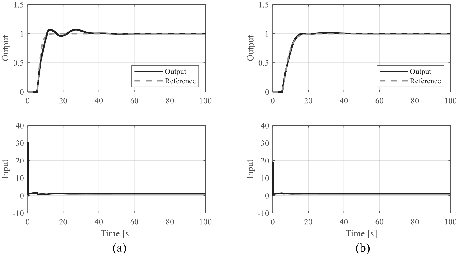
Input and output time series data for the ideal process (a) before and (b) after tuning by Step 2.
Tuned parameters including the reference model for an ideal process system.
[Case 2: Noisy condition]
We verify the proposed method for the process system with noise by assuming a real environment; therefore, the variance of white noise shown in equation (34) is 5 × 10⁻³.
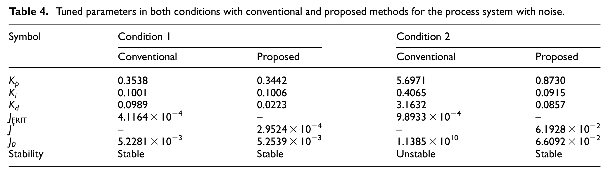
First, we confirm the effectiveness of ID-FRIT with respect to Step 1 of the algorithm. Figure 6(a) shows the time history of the raw and denoised input/output data of the closed-loop system when the initial parameter values are used, and λr is set to 10. The denoised data is obtained using equation (26). Figure 6(b) shows the enlarged view of the output. From the figure, we can obtain the identified dead time of 6.5 s, and this value is used in Step 2 of the algorithm. The denoising method is confirmed to work effectively. Figure 7 shows the time history of the input/output data with the conventional FRIT and the proposed method when the step input under condition 2 is applied to the closed-loop system. The output data of the standard FRIT shown in Figure 7 are divergent. In contrast, in the proposed method, controller parameters that stabilize the closed-loop system are obtained even when model matching cannot be realized. The simulation results are summarized in Table 4, which is used in the discussion section.
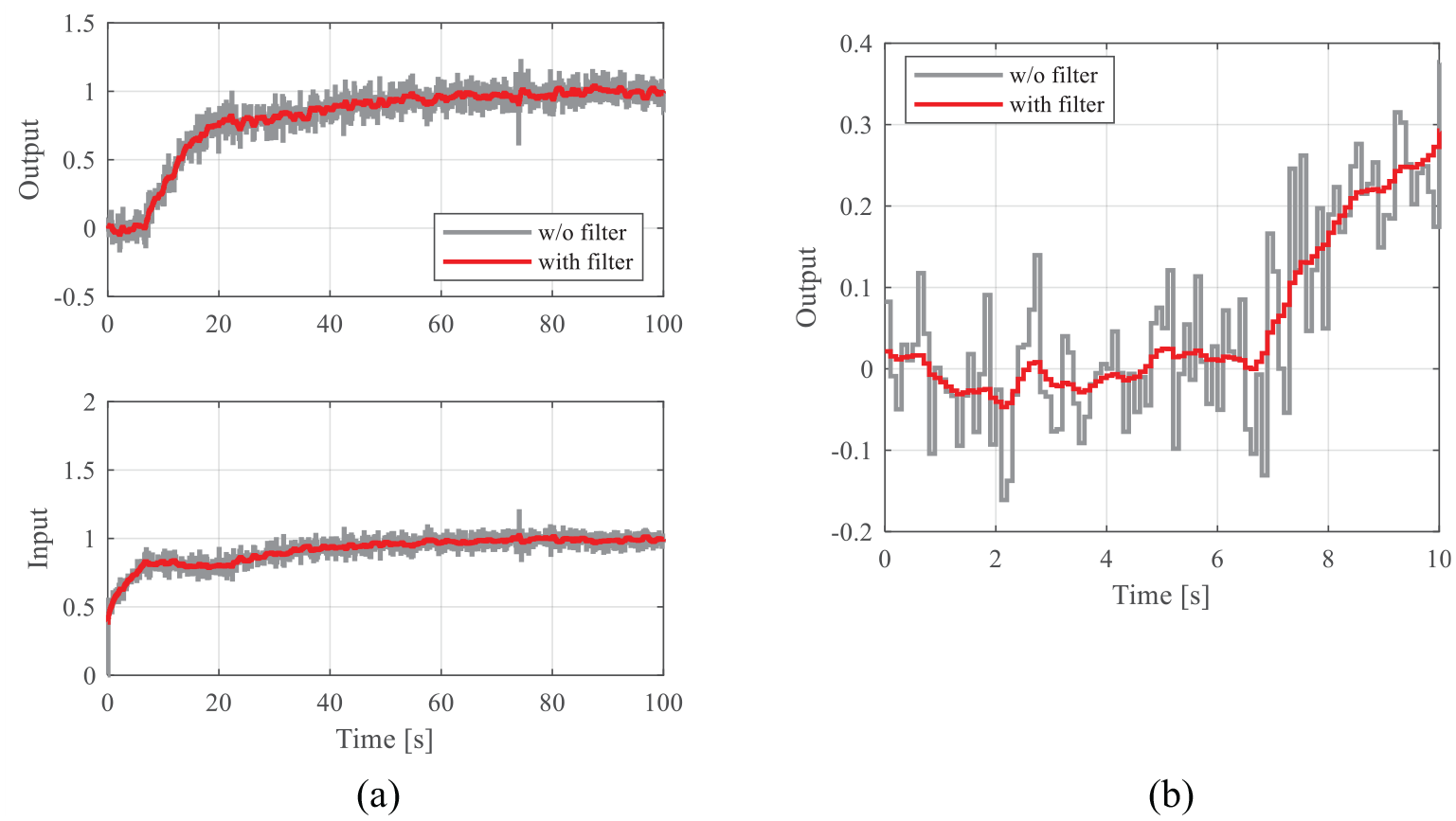
Time-series data without and with the filter using the initial PID gain (λ r = 10): (a) overview of the input and output and (b) enlarged view of the output. Estimated dead time is 6.5 s.
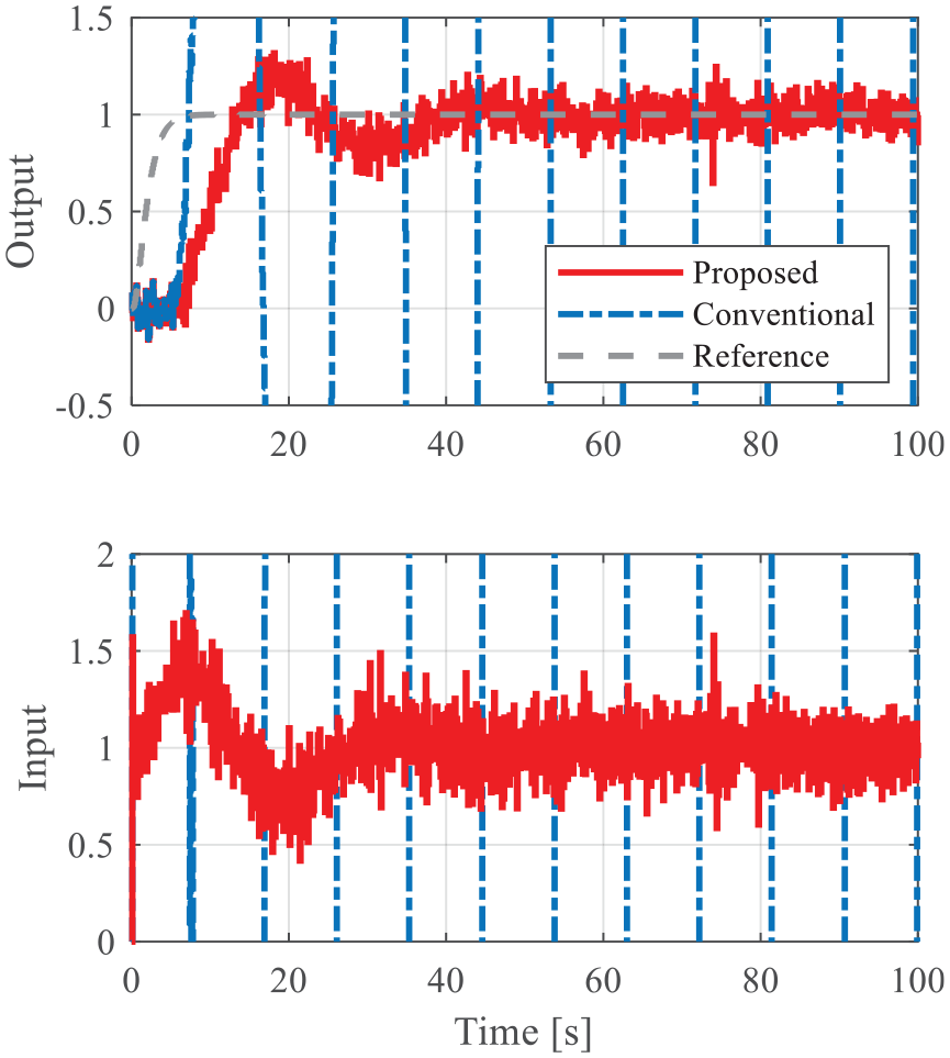
Input and output time series data with the conventional and proposed methods under condition 2 for the process with noise.
Tuned parameters in both conditions with conventional and proposed methods for the process system with noise.
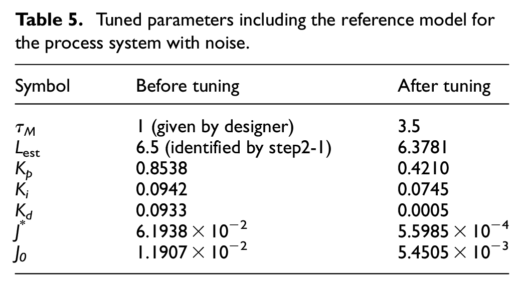
Next, we confirm the effectiveness of the reference-model optimization method with respect to Step 2 of the algorithm. The reference model with a tunable parameter Lest, which is added to equation (30), is used as described in the subsection titled “Method for optimizing the reference model.” Here, we assume that the controlled-object dead time is identified in Step 2-1 as 6.5 s from Figure 6(b). Figure 8 shows the time histories of the closed-loop system using the parameters obtained before and after applying Step 2 of the algorithm. The dead time of the variable reference model before optimization is fixed to 6.5 s to match the conditions before and after applying the optimization algorithm. Figure 8(a) shows the time-series data before applying Step 2 of the algorithm, and Figure 8(b) shows the time-series data obtained after optimizing the responsiveness parameter. In Figure 8(a), the responsiveness parameter is not optimized and the response is vibrational. In contrast, Figure 8(b) shows that the parameter related to the responsiveness of the reference response is optimized. The actual response can follow the reference response under the controller of the specified order. Thus, a response close to the characteristics desired by the designer can be obtained. The simulation results are summarized in Table 5, which is used in the discussion section.
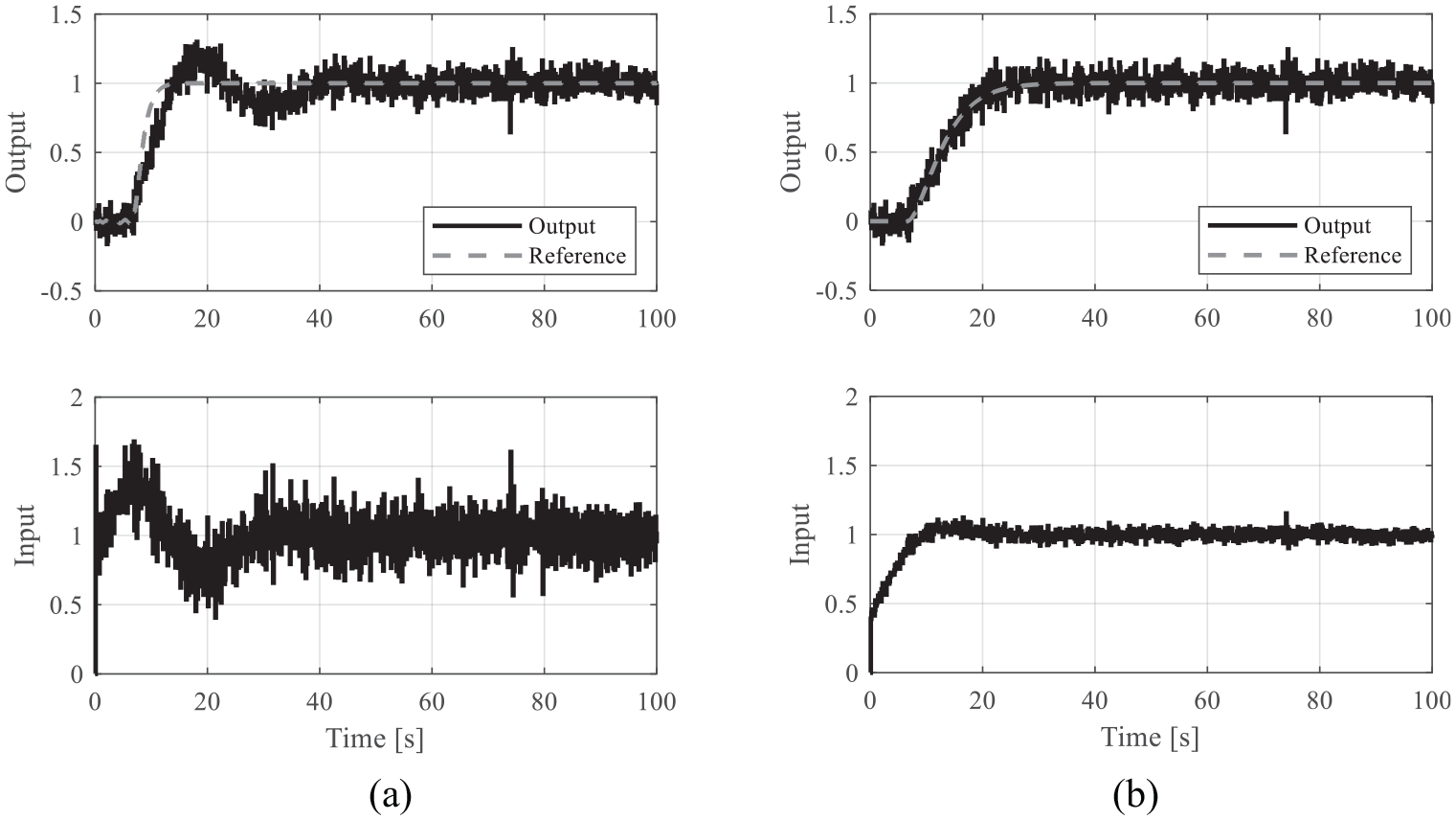
Input and output time series data for the process with noise: (a) before and (b) after tuning by Step 2.
Tuned parameters including the reference model for the process system with noise.
Discussion about system 1
From Tables 2 and 4, the conventional and proposed methods almost provide the same performance when comparing the objective function J0 values under condition 1. This is because the reference model that can easily realize model matching is provided. Under condition 2, model matching cannot be realized because the responsiveness parameter of the reference model is considerably small for the system and the closed-loop system based on the parameters obtained using the standard FRIT is divergent. In contrast, the proposed method results in parameter values that stabilize the closed-loop system. Thus, the proposed method, that is, ID-FRIT, can effectively obtain parameters that can ensure the stability of the closed-loop BIBO. From Tables 3 and 5, the PID gains after Step 2 of the algorithm are smaller than those before the application of this step of the algorithm, and the cost function after Step 2 of the algorithm is better than that before the application of this step of the algorithm. Thus, the control performance and stability can be improved by optimizing the reference model. If the ID-FRIT that considers the detection of the destabilization shown in Step 1 is not used, instability may be encountered in the middle of the algorithm.
Thus, the proposed method is effective because the (i) controller parameters (PID gains) are obtained, which makes the closed-loop BIBO stable. Also, (ii) the characteristics of the closed-loop system are similar to those of the reference model because model matching is realized. Hence, the gain and phase margins of the reference model and the closed-loop stability are almost identical. By obtaining the loop transfer function for the reference model, the gain and phase margins can be predicted even if the controlled-object characteristics are unknown; therefore, the gain and phase margins can be considered. For instance, if the reference model is a binomial-coefficient standard form, a Butterworth standard form, an integral of time weighted absolute error (ITAE) minimum standard form, or the like, then the reference model has a constant phase margin, gain margin, and overshoot rate regardless of the responsiveness parameters. Therefore, the designer can positively consider the gain and phase margins. In this simulation, the reference model is selected to the binomial-coefficient standard form, the poles of which have a real part, as shown in equation (30). Thus, the designer demands characteristics with no overshoot, and the characteristics are realized after Step 2 of the algorithm. With respect to the results obtained using the controlled object without noise, the gain and phase margins of the reference model are 8.301 dB and 63.71°, respectively. In addition, the gain and phase margins of the closed-loop system using the obtained parameters by applying the proposed method are 7.913 dB and 64.63°, respectively. In case of the results obtained with respect to the controlled object with noise, the gain and phase margins of the reference model are 9.867 dB and 65.78°, respectively. Further, the gain and phase margins of the closed-loop system using the obtained parameters by applying the proposed method are 9.811 dB and 64.70°, respectively. Thus, a controller equivalent to the user-defined reference model characteristics can be obtained.
In addition, we provide some supplementary contents. We present the difference between the proposed method and the previous study. 5 In the literature, the controller parameters, the reference-model parameters, and the dead time are tuned without considering BIBO stability. Thus, we cannot predict whether the closed-loop system is stable until the controller is implemented. On the other hand, the proposed method provides BIBO stability and model matching before the controller is implemented. The identification of dead time is not necessary when considering only BIBO. If we consider model matching along with BIBO, we must know the dead time used in Step 2 of the algorithm. However, the proposed method does not require any design parameters except for the dealing noise. The previous study has not described how to deal with noise. Also, the responsiveness parameter of the reference model in the proposed method is smaller than that in the literature. This is because the low-pass filter of the differential term is different. The set value is considered to be appropriate from the results with the noisy condition and previous studies.8,44
Application to system2: Spring-mass system
In this section, we validate the proposed method for a spring-mass system with a response lag and dead time; this system has a time constant faster than that of the process system. Spring-mass systems are often used in many industries. A system with noise is only described because the principle of the proposed method has been confirmed under the ideal process system. The controlled object can be given as follows:
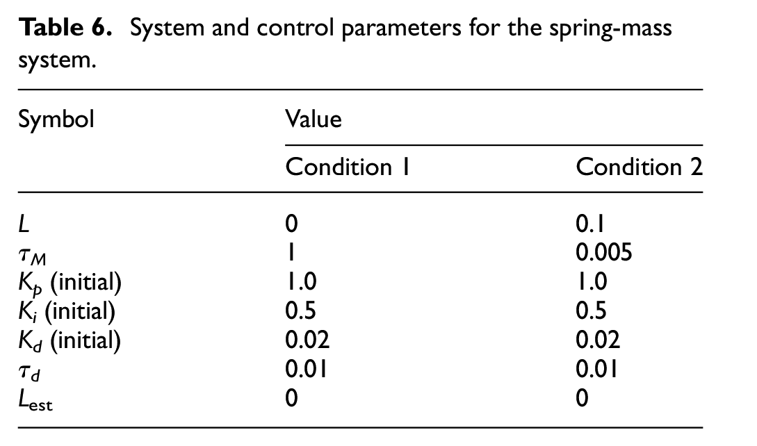
The variance of white noise n is 5 × 10⁻³ when assuming a real environment. The sampling period is 4 ms. The parameter sets are given in Table 6, and the simulation is performed for conditions 1 and 2. In condition 1, model matching is assumed to be possible, whereas in condition 2, model matching is assumed to be not achieved. The conventional and proposed methods are compared in simulations under these two conditions.
System and control parameters for the spring-mass system.
Simulation results under noisy condition
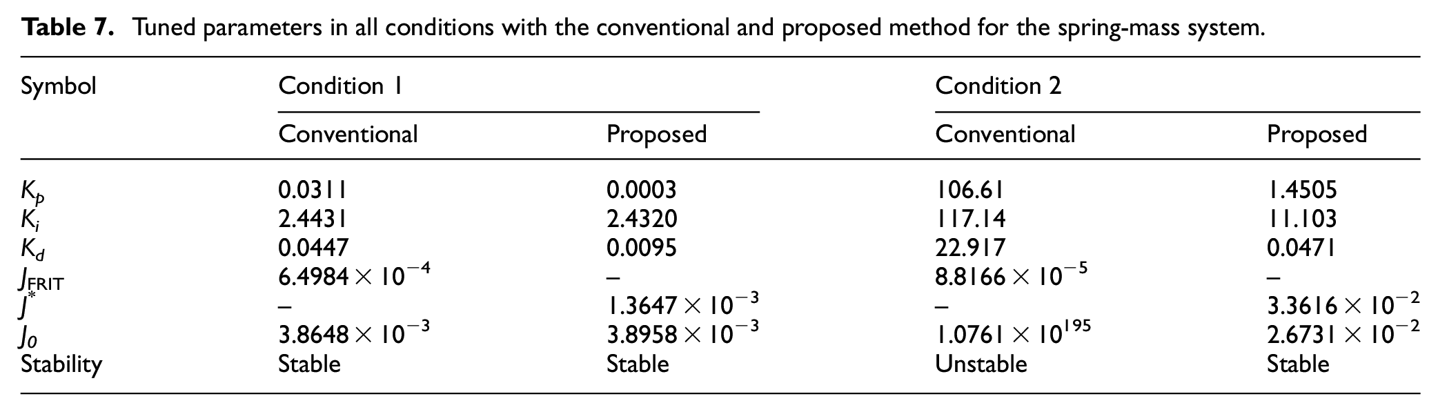
First, we confirm the effectiveness of ID-FRIT with respect to Step 1 of the algorithm. Figure 9(a) shows the time history of the raw and denoised input/output data of the closed-loop system when the initial parameter values are used, and λr is set to 10. The denoised data is obtained using equation (26). Figure 9(b) shows the enlarged view of the output. From the figure, the identified dead time is 0.2 s, and this value is used in Step 2 of the algorithm. Figure 10 shows the time history of the input/output data with the conventional FRIT and the proposed method when the step input under condition 2 is applied to the closed-loop system. From this figure, the output data of the standard FRIT can be confirmed to be divergent. In contrast, in the proposed method, controller parameters that stabilize the closed-loop system are obtained even when model matching cannot be realized. The simulation results are summarized in Table 7.
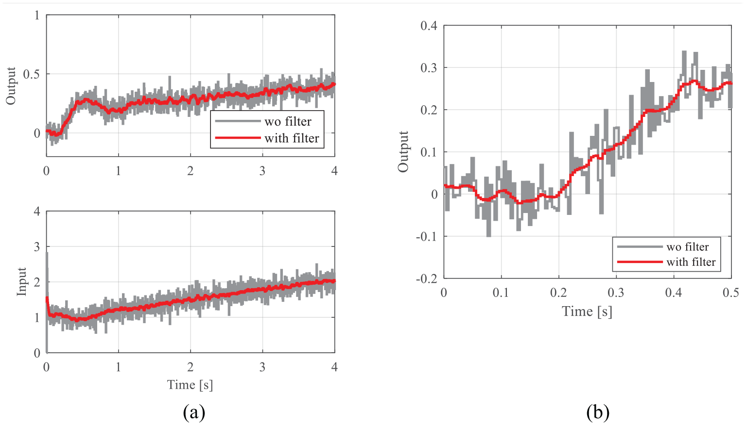
Time-series data used in the optimization without and with the filter under the initial PID gain (λ r = 10): (a) overview of the input and output and (b) enlarged view of the output. Estimated dead time is 6.5 s.
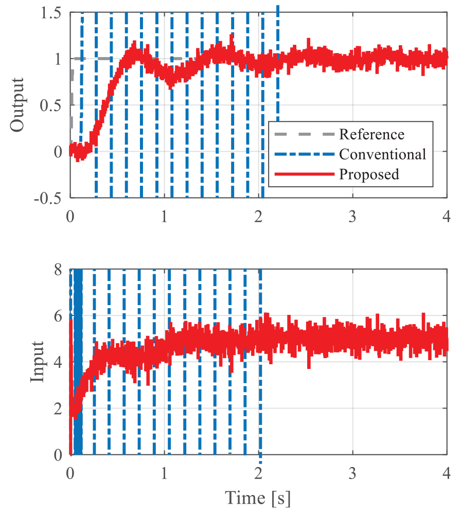
Input and output time series data with the conventional and proposed methods under condition 2.
Tuned parameters in all conditions with the conventional and proposed method for the spring-mass system.
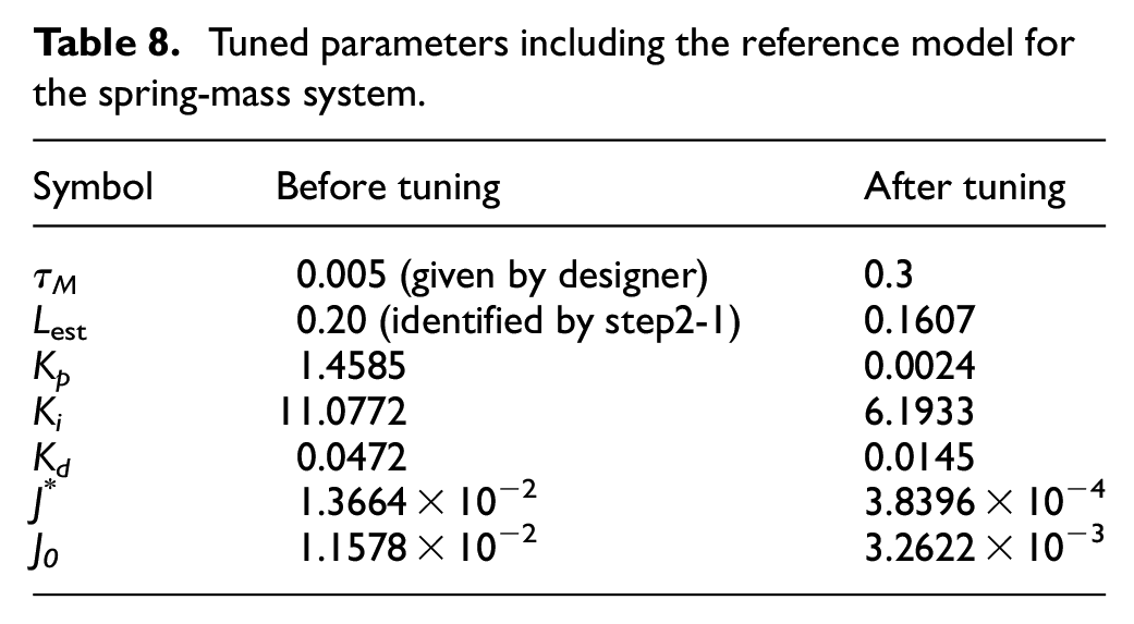
Next, we confirm the effectiveness of the reference-model optimization method using Step 2 of the algorithm. The reference model with a tunable parameter Lest is used as described in the subsection titled “Method for optimizing the reference model.” Here, we assume that the controlled-object dead time is identified in Step 2-1 as 0.2 s from Figure 9(b). Figure 11 shows the time histories of the closed-loop system using the parameters obtained before and after applying Step 2 of the algorithm. The dead time of the variable reference model before optimization is fixed to 0.2 s to ensure that the conditions before and after the application of Step 2 of the algorithm match. Figure 11(a) shows the time-series data before applying the optimization algorithm, and Figure 11(b) shows the time-series data after optimizing the responsiveness parameter. In Figure 11(a), the responsiveness parameter is not optimized and the response is vibrational. In contrast, Figure 11(b) shows that the parameter related to the responsiveness of the reference response is optimized. Further, the actual response can follow the reference response under the controller of the specified order. Thus, a response exhibiting characteristics close to those desired by the designer can be realized. The simulation results are summarized in Table 8.
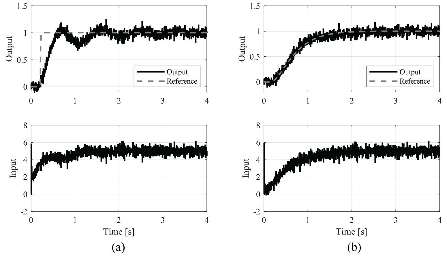
Input and output time series of the experimental data for spring-mass system: (a) before and (b) after tuning by Step 2.
Tuned parameters including the reference model for the spring-mass system.
Discussion regarding system 2
The proposed method is effective with respect to the results obtained by its application to the system because (i) controller parameters (PID gains) are obtained, causing the closed-loop system to become stable. Also, (ii) the characteristics of the closed-loop system coincide with those of the reference model when model matching is realized. After Step 2 of the algorithm, the gain and phase margins of the reference model are 14.67 dB and 70.34°, respectively. Further, the gain and phase margins of the closed-loop system using the obtained parameters by applying the proposed method are 18.00 dB and 84.32°, respectively. The gain and phase margins before the application of Step 2 are 1.676 dB and 22.82°, respectively. Thus, a controller with characteristics equivalent to those of the user-defined reference model can be obtained.
Experimental validation
We verify the proposed method using an experiment. The controlled object is a DC motor, and we obtain the PID gain for speed control. The experimental system is shown in Figure 12. The motor and generator are connected by a rubber. The control input is calculated using a PID controller, and the controlled variable is the rotational speed (generator voltage) of the generator. The sampling period is 40 ms, and the time constant of the derivative filter is 100 ms. The initial PID gains are KP = 2.0, Ki = 0.1, and Kd = 0.005. The dead zone is compensated because the rotation is controlled from the stopped state.
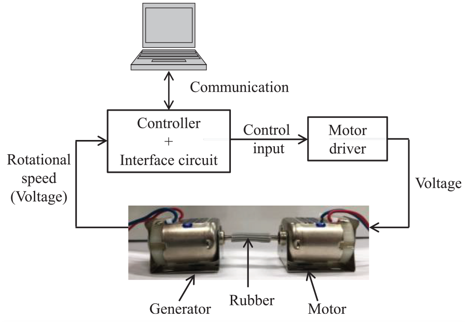
Experimental setup with the motor and generator connected by rubber.
First, we confirm the effectiveness of the ID-FRIT with respect to Step 1 of the algorithm. Figure 13(a) shows the time history of the raw and denoised input/output data of the closed-loop system. when the initial parameter values are used, and λr is set to 5. The denoised data is obtained using equation (26). Figure 13(b) shows the enlarged view of the output. From the figure, we can obtain the identified dead time as 0.12 s, and this value is used in Step 2 of the algorithm. From Step 1 of the algorithm, the PID gains obtained by conventional FRIT are KP = 17.8881, Ki = 20.4399, and Kd = 9.4438. Also, the PID gains obtained by ID-FRIT are KP = 5.1579, Ki = 4.6819, and Kd = 9.4438. Figure 14 shows the time history of the output (generator voltage) and input calculated by the PID controller with the conventional FRIT and proposed method. In this figure, in the proposed method, the closed-loop system is stable even when model matching cannot be realized. In the conventional FRIT, the closed system seems to be not divergent because of the input voltage limitation of the hardware from −5 to +5 V; however, the control input is very large and the PID gains are not appropriate.
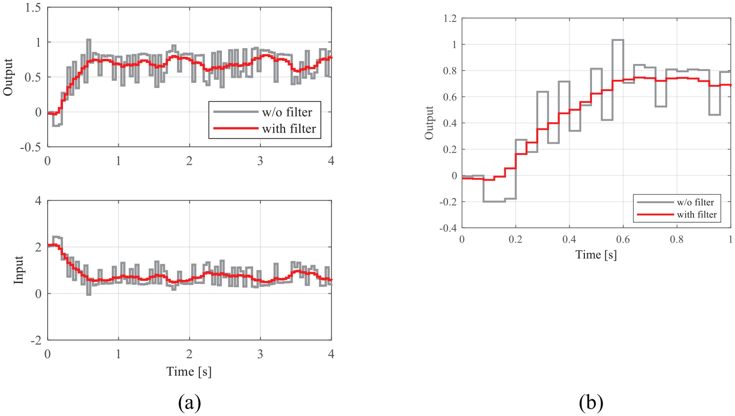
Time-series of the experimental data used in the optimization without and with the filter under the initial PID gain (λ r = 5.0): (a) overview of the input and output and (b) enlarged view of the output. Estimated dead time is 0.12 s.
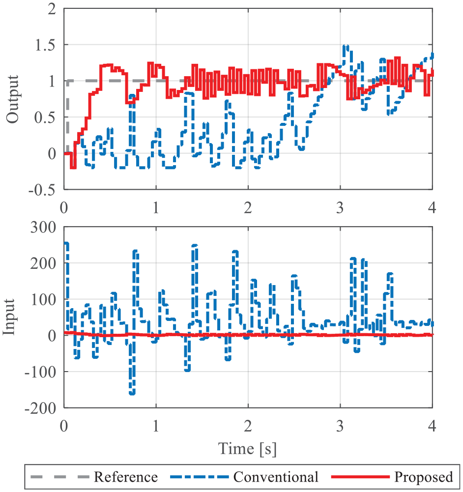
Input and output time series of the experimental data with the conventional and proposed methods under condition 2.
Next, we confirm the effectiveness of the reference-model optimization method using Step 2 of the algorithm. The reference model with a tunable parameter Lest is used as described in the subsection titled “Method for optimizing the reference model.” Here, we assume that the controlled-object dead time is identified in Step 2-1 as 0.12 s from Figure 13(b). The tuned PID gains before applying Step 2 of the algorithm are KP = 2.7890, Ki = 4.2147, and Kd = 0.2823. The dead time of the variable reference model before optimization is fixed to 0.12 s to ensure that the conditions before and after applying Step 2 of the algorithm match. Also, the PID gains and estimated dead time after applying Step 2 are KP = 1.3251, Ki = 1.8455, Kd = 0.0010, and Lest = 0.1198. Figure 15 shows the time histories of the closed-loop system using the parameters obtained before and after applying the above algorithm. Figure 15(a) shows the time-series data before applying Step 2 of the algorithm, and Figure 15(b) shows the time-series data after the optimization of the responsiveness parameter. In Figure 15(a), the responsiveness parameter is not optimized and the response is not close to the reference response. In contrast, Figure 15(b) shows that the parameter related to the responsiveness of the reference response is optimized, and the actual response can follow the reference response. Thus, the parameters obtained using the proposed method provide BIBO stability and model matching.
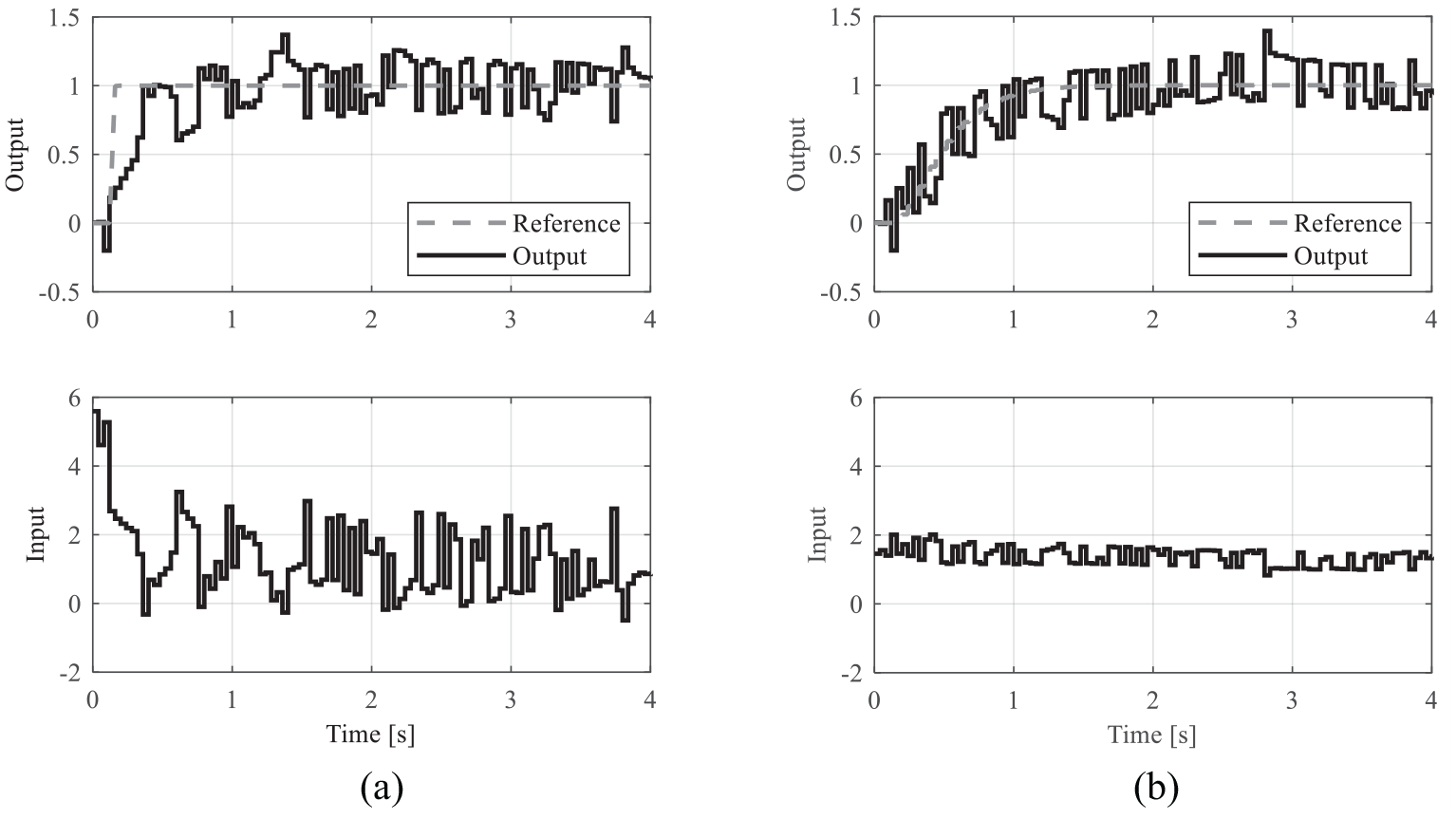
Input and output time series of the experimental data: (a) before and (b) after tuning by Step 2.
Conclusion
In this study, we propose a direct tuning method for the feedback controller parameters based on a fictitious reference signal that considers BIBO stability and model matching without repeating experiments. The proposed method includes a two-step algorithm. In the first step, the BIBO stability of closed-loop system is satisfied. A transfer function, the input and output of which are a fictitious reference signal and a controlled-object response, respectively, is identified in the time domain to obtain pole information. Thus, we can obtain the parameters that make the closed-loop system BIBO stable. In the second step, model matching between reference model and closed-loop system is considered. If model matching is achieved, the characteristics of the reference model almost match those of the closed-loop system, including the gain and phase margins. The reference model parameters are automatically tuned using the proposed algorithm for model matching. Thus, BIBO stability and model matching can be considered in the two-step algorithm. Moreover, the design parameters are not influential apart from noise. These features allow the easy application of this method. Thus, many engineers can easily use this method. Two simulations and an experiment were performed on a system with dead time to verify the effectiveness of the proposed two-step method. Results showed that the conventional standard FRIT and the proposed method result in optimal controller parameters when model matching is possible. However, when model matching is impossible because of an inappropriate reference model, the closed-loop system using the controller parameters obtained with the standard FRIT is unstable, whereas the proposed method can be used to obtain optimum control parameters without destabilizing the system. In addition, model matching was realized by reference model optimization. Thus, the parameters obtained using the proposed method provide BIBO stability and model matching. In the future, we will examine online model-free control, including adaptive control, to nonlinear systems because our method is obtained in the time domain without information about the controlled-object model.
Footnotes
Appendix
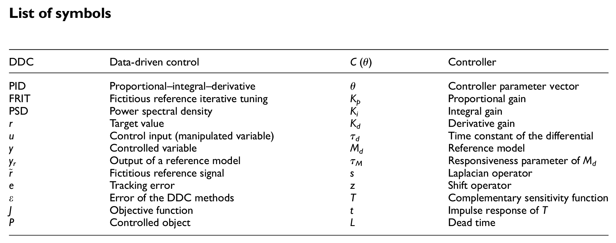
| DDC | Data-driven control | C (θ) | Controller |
|---|---|---|---|
| PID | Proportional–integral–derivative | θ | Controller parameter vector |
| FRIT | Fictitious reference iterative tuning | Kp | Proportional gain |
| PSD | Power spectral density | Ki | Integral gain |
| r | Target value | Kd | Derivative gain |
| u | Control input (manipulated variable) | τd | Time constant of the differential |
| y | Controlled variable | Md | Reference model |
| yr | Output of a reference model | τM | Responsiveness parameter of Md |
| Fictitious reference signal | s | Laplacian operator | |
| e | Tracking error | z | Shift operator |
| ε | Error of the DDC methods | T | Complementary sensitivity function |
| J | Objective function | t | Impulse response of T |
| P | Controlled object | L | Dead time |
Authors’ Note
Itsuro Kajiwara is now not affiliated with Division of Human Mechanical Systems and Design, Hokkaido University, Sapporo, Hokkaido, Japan.
Declaration of conflicting interests
The author(s) declared no potential conflicts of interest with respect to the research, authorship, and/or publication of this article.
Funding
The author(s) received no financial support for the research, authorship, and/or publication of this article.