
Abstract
Industries are increasingly adopting automatic and intelligent manufacturing in production lines, such as those of semiconductor wafers, optoelectronic devices, and light-emitting diodes. For example, automatic robot arms have been used for pick-and-place workpiece applications. However, repairing automatic robot arms is time-consuming and increases the downtime of equipment and the cycle time of manufacturing. In this study, various machine learning (ML) models, such as the general linear model (GLM), random forest, extreme gradient boosting, gradient boosting machine, and stacked ensemble, were used to predict the maximum Cartesian positioning shift (i.e. the maximum eccentric distance) in the next handling time period (e.g. 1 min). A charge-coupled-device-based fault diagnostic system was developed to measure the critical positions of the robotic arm when transferring wafers. A novel data augmentation method was used to determine the correlation parameters in the dataset for the ML models. The prediction error for each algorithm was determined using the root mean square error (RMSE). The results revealed that the GLM exhibited the lowest prediction errors. The RMSEs of the GLM were 0.024, 0.032, and 0.046 mm for 3421 pickups, the last 1000 pickups, and 100 pickups, respectively, for the prediction target. Thus, the GLM is a promising model for predicting the task failure of wafer-handling robotic arms.
Keywords
Introduction
An industrial robot is a programmable piece of mechatronic equipment that is generally used in production lines to perform repetitive or dangerous tasks automatically for ensuring high fabrication quality. For instance, numerous robots are used in semiconductor wafer, optoelectronic device, and light-emitting diode fabrication industries to perform various tasks. Typically, triaxial robotic arms are placed at etching, deposition, and photolithography stations to pick and place wafers between cassettes with high accuracy, repeatability, and reliability. However, repairing robotic arms is time-consuming and considerably increases the downtime of equipment and the cycle time of manufacturing. 1 Figure 1 displays a real-world example in which three wafers were dropped by a robotic arm when transferring them. The subsequent maintenance procedures were complex and time-consuming. First, an engineer collected all the damaged pieces from the working area. Then, the failed components of the robot were inspected and repaired. Finally, the handling process was restored, and a trial run was performed to ensure that the robotic arm was repaired. The task failure of handling robots is the main cause of yield loss in semiconductor manufacturing. Therefore, a reliable method for reducing the occurrences of task failures should be developed urgently to improve the availability of handling robots. 2
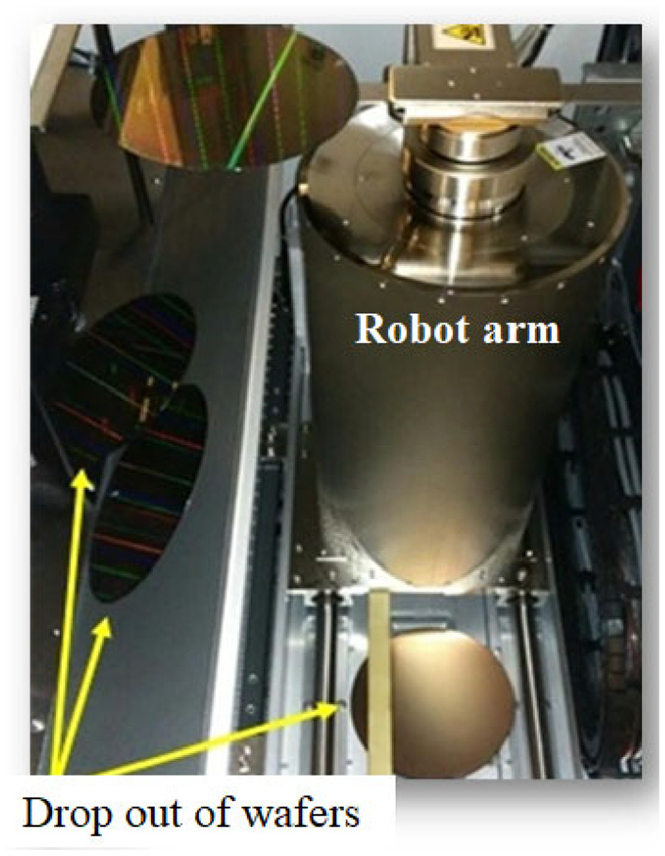
Wafers dropped by the robotic arm.
In 1993, Ntuen and Park 3 proposed a system-level methodology that involves using a reliability block diagram (RBD) to evaluate the reliability of certain robots. The module was divided into mechanical, sensor, and control modules in series. Subsequently, Korayem and Iravani 4 applied failure mode and effect analysis (FMEA) and quality function deployment to improve the reliability and operational quality of the 3P and 6R robotic arms. Yamada and Takata 5 and Lueth et al. 6 investigated the optimal factors to reduce the operational failures of robotic arms when performing specific tasks. Conventional reliability analysis was performed in the aforementioned studies to evaluate the failures of various types of robot arms for certain tasks. 7 The errors were instrumental in the development of effective solutions to improve the operational reliability. However, these solutions are only effective for certain work conditions. To address this problem, proactive reliability assessment methods or prognostics and health management (PHM or predictive maintenance) have been used in real-time situations for equipment maintenance. In most cases, PHM is used to predict the residual useful life (RUL). This model actively and recursively predicts and updates information periodically regarding the monitored critical parameters. Therefore, the state of health (SOH) of assets can be determined. Furthermore, the model assists engineers in determining the assets’ best time to maintenance (BTTM).
Proactive models are categorized into model-based, data-driven, or hybrid models. The data-driven model mainly relies on the Wiener or Gamma stochastic process to determine the performance degradation routes for devices under test (DUTs).8–13 The lifetime of a product is defined as the time when the specific value of the product first passes the critical first passage time. Machine learning (ML)-based data-driven models have been applied to predict lifetimes and monitor the SOH of critical products.14–19 These models use neural networks or other ML algorithms to determine the aging behavior of assets and achieve high prediction accuracy. Although proactive techniques effectively update the RUL, the prediction frequency of these techniques for some applications, especially in the case of fast degradation or immediate failure behaviors, is unreliable. For instance, when performing in situ prognostics of electronics, proactive techniques achieved the worst prediction accuracy of short circuits because the transition from the abnormal state to the failure state was fast. 20 Furthermore, the RUL is not adequate for predicting discrete and repetitive task failures of handling robots because the success of the next one handling cycle is more concern than the prediction of residual useful life. For a real situation, the specimen drops on the current pick-up cycle but the prediction of RUL displays that the failure will occur on many handling cycles later. Thus, it is necessary to develop effective methodology to predict the probability of success for the next one pick-up cycle of robotic arms.
In this study, a proactive data-driven methodology based on ML was developed to evaluate task reliability, that is, the maximum Cartesian positioning shift in the next time interval, which is the main parameter related to failure. A charge-coupled-device-(CCD)-based fault diagnostic system was used to capture pictures of the pickup motion of robotic arms. The X–Y position of the arm was then determined from the images by using a vision identification software. Considering the requirement of reliable, cost-effective, and precise prediction quality in smart manufacturing, the supervised statistical-based machine learning methodologies regarding with the general linear model (GLM), random forest (RF), extreme gradient boosting (XGB), gradient boosting machine (GBM), and stacked ensemble (SE) were applied to predict the maximum Cartesian positioning shift (i.e. the maximum eccentric distance) in the next 1 min time interval. To improve the prediction accuracy, a novel data augmentation method that combines root cause analysis and statistical parameter calculation was used to determine the failure causation and parameter correlation. Uncertainty analysis was performed by calculating the root mean square error (RMSE) for all algorithms to select the best ML model (i.e. the model with the lowest RMSE).
Wafer-handling diagnostics and prognostics system
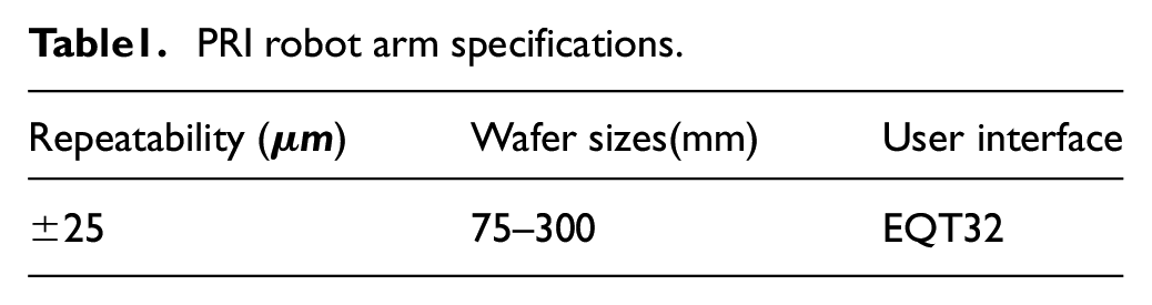
Figure 2 displays the layout of the T-axis, R-axis, Z-axis, and Table 1 presents the specifications of the robotic arm. This triaxial robot arm is typically used in semiconductor production lines to pick wafers from the cassette and place them on the chuck for manufacturing. On completion of the manufacturing process, the robotic arm removes the wafers from the chuck and places them back on the cassette. Typically, the T (θ)-axis denotes the rotation of the arm, the R (radial)-axis denotes the reach and retraction ability of the arm, and the Z (vertical)-axis denotes the vertical movement. Figure 3 displays the robot fault diagnostics system that consists of a wafer-handling robotic arm, chucks, cassettes with wafers, a CCD camera module, and a laptop that is used as the control unit for the system.
21
A visual identification software program was used to record and translate pixels of the photograph to X–Y position data. In the diagnostic process, first, all the process parameters were decided and the initialization process was performed by home-positioning the robot. Second, when the robot arm began its first task to deliver the test wafer to the chuck, the CCD camera captured the motion. The software program recorded the geometry of the wafer and computed the central point of the wafer
PRI robot arm specifications.
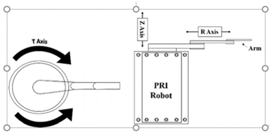
Handling robot and the T-axis, R-axis, and Z-axis.

Fault diagnostic system of the robotic arm 21 : (a) framework and (b) system in operation
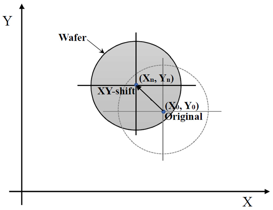
Pick-up position shift.
The raw data have to be preprocessing before they were used as input dataset for machine learning. First step of doing data preprocessing was to calculate the XY-shift, and the second step was to perform the data augmentation shown in the later section 3.4. In the prognostic model, the threshold value is defined by the critical eccentric distance that precedes failure. Thus, the maximum acceptable limit of the position deviation during the wafer-handling tasks is determined. The eccentric distance is calculated using the following expressions:
ML techniques
Many novel ML algorithms have been developed for various applications. For instance, deep neural-based networks provide state-of-art frameworks for text-independent speaker verification, object detection, and media recommendation. 22 However, conventional algorithms corresponding to bagging, boosting, decision trees, and linear-based regression methodologies provide comprehensive formulations and case studies to solve problems in industries and businesses. Furthermore, an ensemble of multiple statistic-based learning algorithms is used to obtain superior predictive performance to that of any of the constituent learning algorithms. 23 In this study, measurement data were collected from the wafer-handling diagnostics and prognostics system and used as the input of five ML models, namely the GLM, SE, RF, GBM, and XGBoost. The following subsections briefly introduce these learning algorithms
SE
SE is a supervised ensemble ML algorithm in which the optimal combination of a collection of prediction algorithms is obtained through a stacking process. SE enables regression, binary classification, and multiclass classification by using a select algorithm pool including GLM, GBM, RF, deep learning, and XGBoost. Wolpert introduced the SE method in the early 1990s 24 and developed an approach to combine several base predictors into a high-level model for increasing prediction accuracy. Subsequently, the SE method was developed several times and is now called super-learner regression25–27 or stacked regression. 28 A k-fold cross-validation process is generally applied to determine an optimal weighted combination of predictions from multiple learning algorithms. Optimality is defined using a specified objective function, such as the minimum RMSE for continuous data or the maximum area under the receiver operating characteristic curve for discrete data. Super-learner regression is a powerful tool for estimating complex real-world relationships while avoiding unsubstantiated parametric assumptions and overfitting to improve predictive performance. 29 The general super-learner algorithm for prediction is described in accordance with the research of van der Laan et al. 27 The learning dataset is defined as follows:

where Y is the outcome of interest and C is a p-dimensional set of covariates. The objective is to evaluate the function
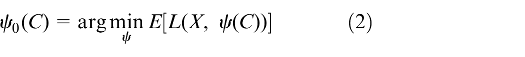
where the loss function is typically the square of the error loss (
Tree-based ensemble machines
RF is a popular supervised data-mining technique that comprises decision trees and uses both bootstrap aggregation (bagging) and random variable selection to construct trees. This method was introduced by Ho. 30 He used a method to concordantly grow trees in random subsets of features. When growing trees to form a forest, the training data were projected into a randomly selected subspace involving each node or tree. Then, the randomized nodes were optimized to make a proper decision. Breiman 31 extended this method of combining node optimization and bagging techniques to construct a forest with uncorrelated trees. This process is similar to a classification and regression tree procedure. The out-of-bag error was used as an estimate of the generalization error, and variable importance was measured through the permutation process. For regression, the prediction produced by each tree in the forest was summarized and processed using an averaging method. Subsequently, Breiman introduced gradient boosting techniques to develop various tree models, such as the gradient-boosted regression tree and GBM. GBM combines multiple weak trees and creates a strong learner to optimize predictive performance.
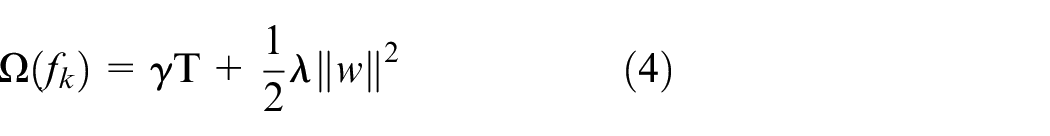
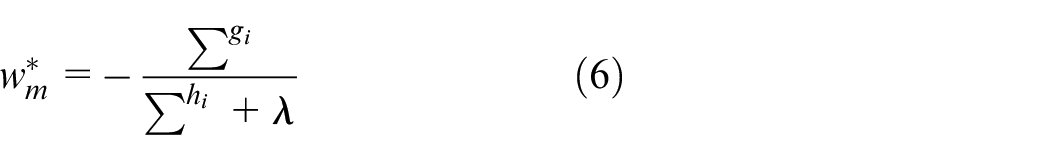
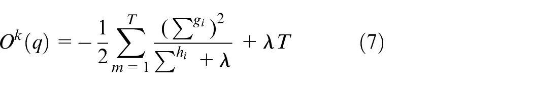
XGBoost was introduced by Chen in 2014. Subsequently, XGBoost became a popular and powerful ML tool because it requires limited effort for data preprocessing and has few hyperparameters that require tuning. XGBoost exhibits superior data learning and antinoise ability to solve complex classification and regression problems. Furthermore, XGBoost is easier to implement than artificial-neural-network-based algorithms are and can help decision makers clearly understand the working process and outcome generation in the predictive model. When training the model, the training error of the previous tree is trained as the learning goal of the current tree, and the results of multiple trees are overlapped to obtain the final result. To obtain superior model capability, the optimal splitting node must be determined to minimize the objective function
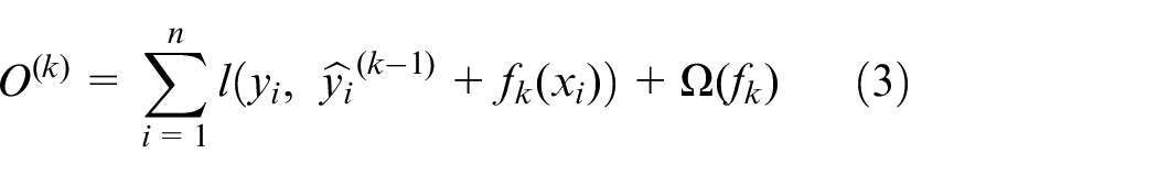
where n is the number of training samples;
where
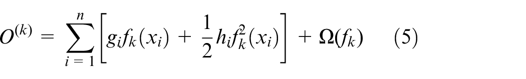
where
GLM
GLMs were introduced by Nelder and Wedderburn. 33 GLMs are a combination of linear and nonlinear functions associated with a distribution of the exponential family involving normal, inverse normal, binomial, Poisson, gamma, and logistic functions. The GLM consists of the following three components 34 :
Random component: n values of the response variable (y1, …, ym)
Systematic component: a linear composition for the regression model of
Link function: a monotone and differentiable function g, which connects the random and systematic components and relates the response variable mean (μ) with the linear structure of
Each distribution has a unique link function. For instance, the widely used distribution for the estimation of air pollution health impacts is the Poisson function denoted by Y ∼ Poisson (μ).
35
Its link function is η = log(μ); thus,

where Y = y1, …, ym,
Data review and augmentation
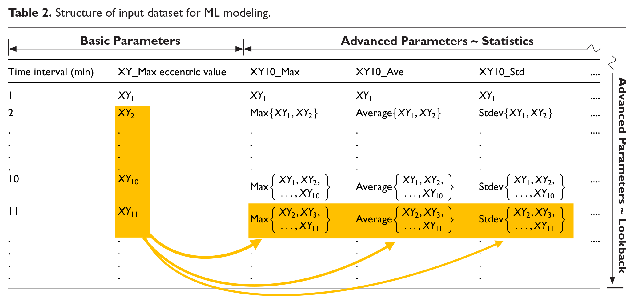
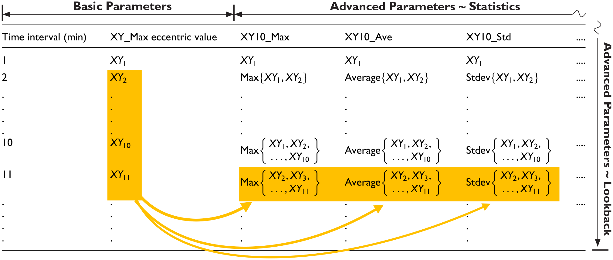
Figure 5 displays the variations in the maximum eccentric distance with one-minute time intervals. The data were collected from the XY-shift measurements. The duration of the time-series data was 17,921 min, of which 14,500 min (80%) were used for training and 3421 min (20%) were used for testing (prediction). The failure threshold was set as 1 mm. Failure occurred in the 17,921st min, with the maximum eccentric distance being 1.132 mm. The profile of time-series data regarding the maximum eccentric distances during 17,921 min pick-ups exhibited a randomly vibrated-like curve that is great challenge for data-driven ML modeling. Additional labels had to be generated to identify the latent features, which resulted in the fast and complex variation of the maximum eccentric distance profile. In this study, a novel data augmentation method was developed by combining root cause analysis (RCA) with statistical parameter calculation to determine the causation and correlation of data for ML-based modeling. The RCA was performed through FMEA to find the error source of positioning shift. The results revealed that teeth wear of motor drive belts is a major failure mechanism to conduct the failure mode of positioning shift. Thus, the advanced parameters were created according to the measured data to enhance the wear-induced degradation behavior of the belt. Table 2 presents the parameters of input dataset for ML modeling. The time interval of 1 min and the maximum value of XY-shift among 1-min pick-ups denoted by XY_Max are basic parameters from measurements. Different lookback sizes and statistic-based data augmentations are advanced parameters described in the following text.
Structure of input dataset for ML modeling.
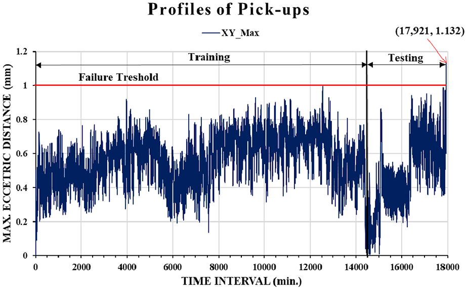
Profile of XY_Max with 1-min time intervals.
First, various lookback sizes were used for the time-series dataset to simulate the accumulated wear behavior of the belt in the physical domain. The parameters of different “lookback” sizes at each time interval of the dataset are going to create various accumulated quantities of wear for machine to learn the critical failure behavior of the belt. This behavior is defined by the number of recent data points to be used when predicting each future value in the time-series domain. The lookback size n for the present data denotes that the maximum eccentric distance (XY_Max) for recent past n-minute intervals, including the present time interval, is named XYn_Max, n = 1, ..., i. For instance, XY10_Max denotes the “maximum value” of XY_Maxs at the present minute interval where it is selected by looking back the values of XY_Maxs at recent past 10 1-min intervals, including the present time interval. In this study, lookback sizes of 10, 30, 50, and 100 were used.
Second part of advanced parameters was the statistic-based data augmentation detailing the average, and standard deviation for XY_Max considering look size n. For instance, “XY10_Ave” shown in Table 2 denotes the “average value” of XY_Maxs at the present minute interval where it is selected by looking back the values of XY_Maxs at recent past 10 1-min intervals, including the present time interval. Figure 6 displays the comparison of XY_Max and XY10_Max profiles in the maximum eccentric distance with 1-min time intervals. It can be seen that XY_Max and XY10_Max represent the almost same variety of maximum eccentric distances during the whole time intervals, but the values of XY10_Max are greater or equal to ones of XY_Max to reveal higher probability of dropping wafer. From the maintenance point of view, it is better consideration to use XY10_Max as a prognostic parameter. In this study, XY10_Max was selected to be the prediction function (target) to determine the maximum eccentricity in the next 1 min time interval.
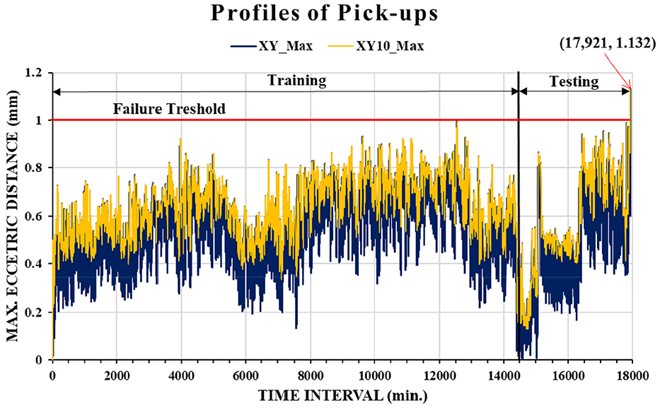
Comparison of XY_Max and XY10_Max profiles.
Results and discussion
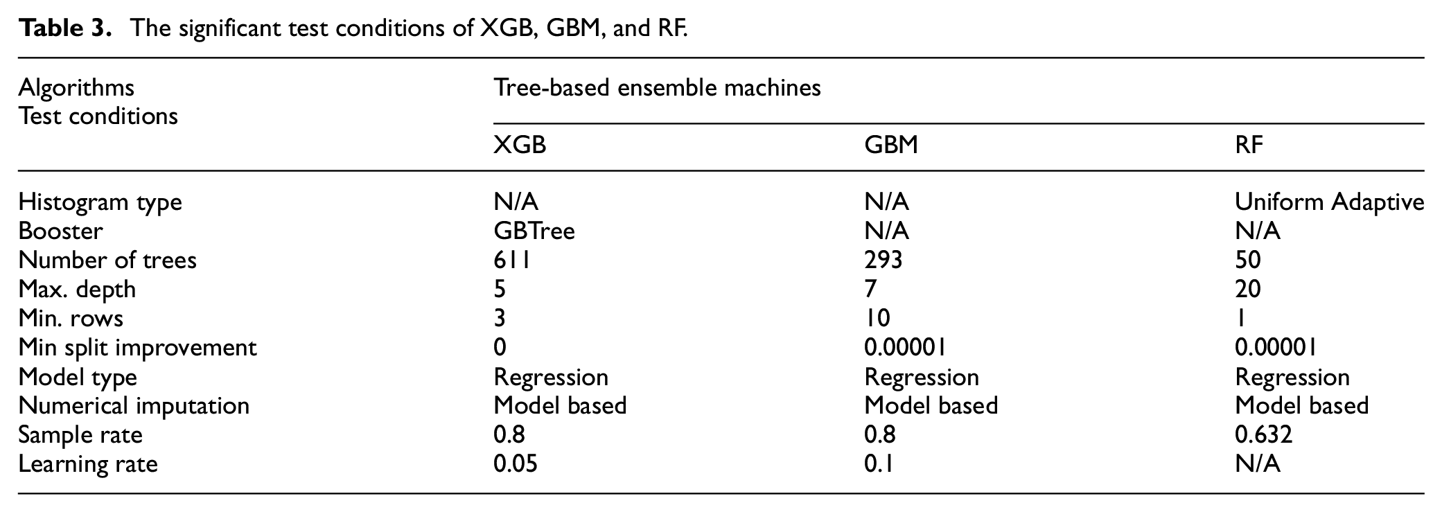
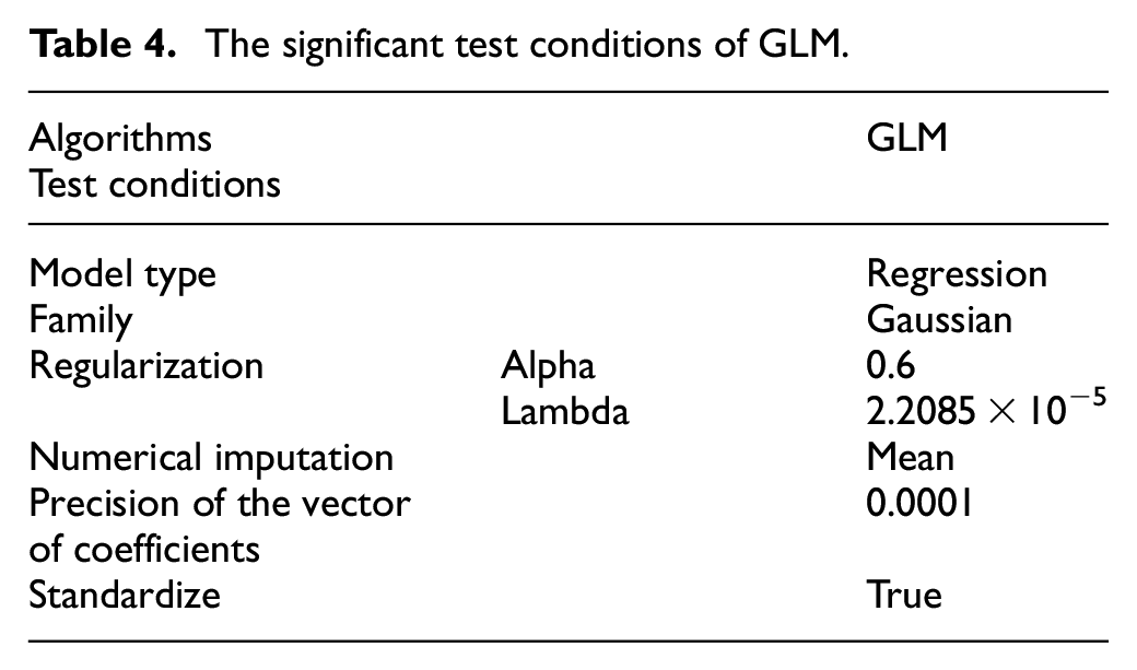
Table 3 displays the significant test conditions of tree-based ensemble machines regarding with XGB, GBM, and RF. Compared to the GBM and RF, XGB used the largest number and the smallest max. depth of trees. XGB and GBM also represent the higher sample rates than that of RF. Table 4 shows the significant test conditions of GLM. The Gaussian was used as the family and link distribution, and regulation was applied to solve problems with overfitting. Besides, the test conditions of SE were quite simple that the GLM was selected as a meta learner, and other four algorithms were ensembled to obtain the optimal combination. Table 5 presents the training evaluation by five-fold cross validations for regression. It can be seen that GLM represents the best results of validation regarding with the average 0.9999 and standard deviation 0.0000. However, these five algorithms demonstrate the premium results for data training. They have already to predict the target (XY10_Max) for the test dataset.
The significant test conditions of XGB, GBM, and RF.
The significant test conditions of GLM.
The training evaluation by 5-fold cross validations.
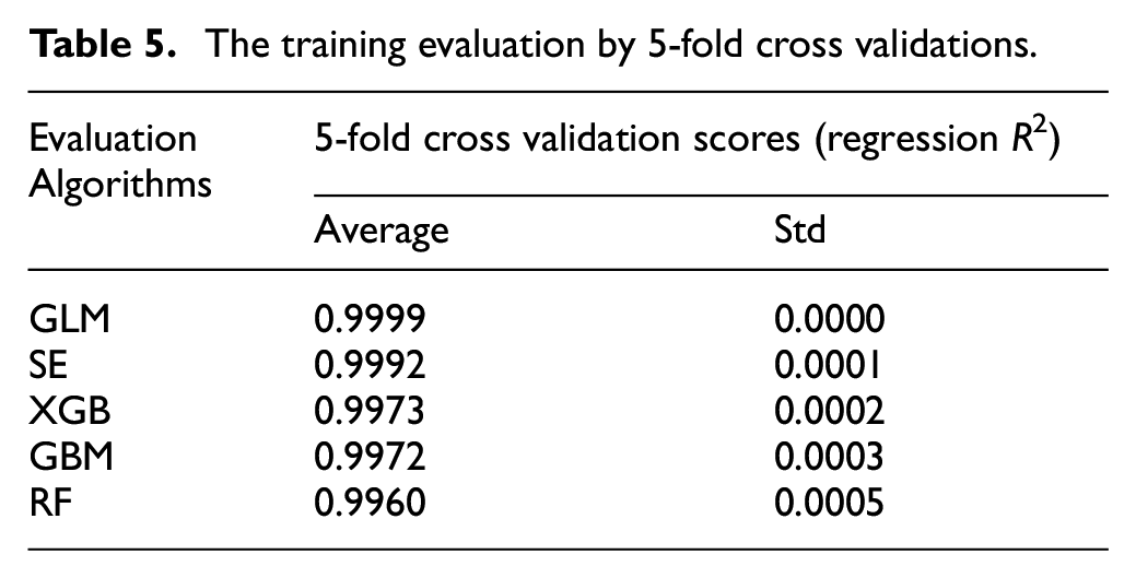
Figure 7 illustrates the prediction profiles of the five ML algorithms for XY10_Max. These ML models satisfactorily predicted the target because all profiles of prediction were similar to that of the real data. The prediction accuracy of the ML models was evaluated using the RMSE (Figure 8), which is a standard measure for determining the error of an ML model in predicting quantitative data. In this study, 3421 pickups (the entire test data), the last 1000 pickups, and the last 100 pickups were used to evaluate each algorithm. The GLM achieved the best prediction with the lowest RMSEs (average RMSE was 0.034 mm) for the aforementioned three conditions. The GBM provided the next best prediction with an average RMSE of 0.049 mm. The combination of the linear and nonlinear functions with the exponential family in GLM provided a flexible and fast response to the randomly vibrating profile, which resulted in high prediction accuracy. Furthermore, if the number of weak trees is increased to optimize predictive performance in the GBM, results similar to those of the GLM may be obtained. The remaining algorithms also exhibited high RMSEs because all the predictions are close to the prediction function XY10_Max. It can be seen in Figure 7 that they are likely to follow the “tempo” of vibration-like profile.
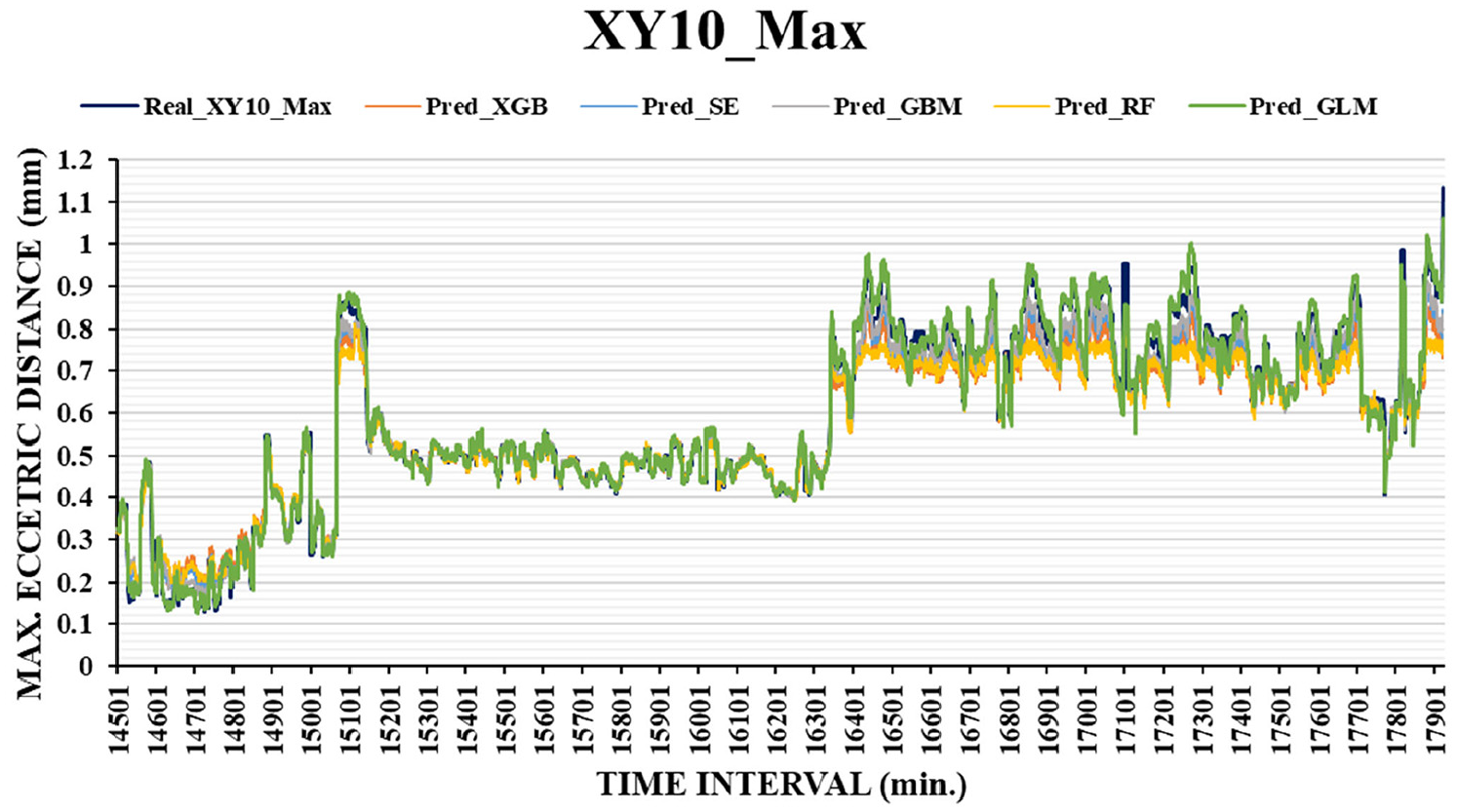
Prediction profiles of the five ML algorithms for XY10_Max.
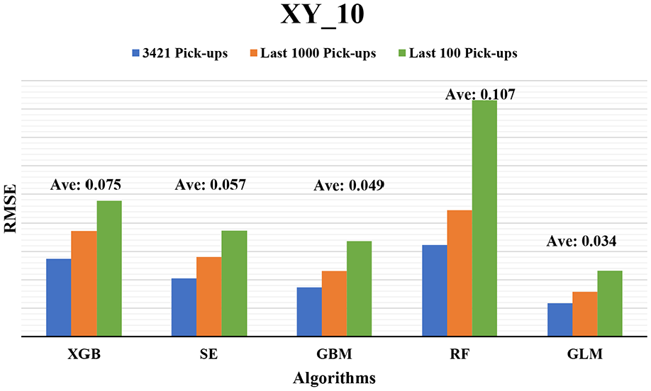
Prediction accuracy of the five ML models in terms of the RMSE.
Figures 9 and 10 present the prediction profiles of the five ML algorithms for the last 1000 and 100 pickup motions, respectively. Unlike other profiles, the prediction profile of the GLM is nearly located on top of the real data profile, which indicates that most of the XY10_Max values were marginally overpredicted (i.e. the predicted value is great than the real value). Therefore, the GLM is a conservative ML model for the prediction of maximum eccentric distances. As mentioned previously, it is better consideration to maintenance because the expectation of good prediction should be more conservative to stop the machine prior to failure. In this study, task failure occurred in the 17,921st pickup whose value of maximum eccentric distance (1.132 mm) was great than the one of failure threshold (1 mm), and only the GLM provided a successful prediction in the previous time period (predictive value was 1.063 mm). Before17,921st pickup, only GLM provided a failure prediction at 17,880st pickup, which the predictive value was 1.023 mm and real value is 0.972 mm. Although it was a little early for predicting failure, it provided a significant warning information to notice that the failure would occur in the near future. In summary, the GLM is the best ML model for task failure prediction.
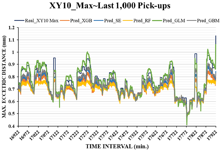
Prediction profiles of the five ML algorithms for the last 1000 pickups.
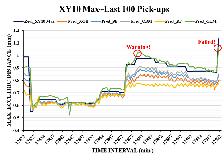
Prediction profiles of the five ML algorithms for last 100 pickups.
Conclusions
Proactive reliability assessment by using ML is a promising method for evaluating the SOH of assets in operation and thus determine the BTTM of the assets. In this study, the GLM, RF, XGB, GBM, and SE were used to predict the task failure in terms of the maximum Cartesian positioning shift (i.e. the maximum eccentric distance) in the next handling time period (e.g. 1 min). The comparative prediction results revealed that the GLM exhibited the lowest prediction error (RMSE) and was the only model to successfully predict failure. Therefore, the GLM is a promising model for predicting task failures for wafer-handling robotic arms. In the future, numerous ML-based devices can be used on production lines to predict the maximum eccentric distances for wafer-handling robotic arms.
Footnotes
Declaration of conflicting interests
The author(s) declared no potential conflicts of interest with respect to the research, authorship, and/or publication of this article.
Funding
The author(s) disclosed receipt of the following financial support for the research, authorship, and/or publication of this article: This research is supported by Ministry of Science and Technology of Taiwan (Grant No. 107-2622-E-018-004-CC2 and 106-2622-E-018-001-CC2).