
Abstract
Both speed and accuracy are key issues in nano-positioning. However, hysteresis existing in piezoelectric actuators severely reduces the positioning speed and accuracy. In order to address the hysteresis, a U-model based active disturbance rejection control is proposed. Based on the linear active disturbance rejection control, a controlled plant is dynamically transformed to be pure integrators. Then, according to the U-model control, a common inversion is obtained and the controlled plant is converted to be “1.” By integrating advantages of both linear active disturbance rejection control and U-model control, the U-model based active disturbance rejection control does promote the reference tracking speed and accuracy. Stability and steady-state error of the close-loop system have been analyzed. Phase lag between the system output and the control input has been effectively eliminated, and the phase-leading advantage of the U-model based active disturbance rejection control has been confirmed. Experimental results show that the U-model based active disturbance rejection control is capable of achieving faster and more accurate positioning. Remarkable improvements and practical realization make the U-model based active disturbance rejection control more promising in nano-positioning.
Introduction
Nanotechnology is the science of understanding and controlling the matter at dimensions of 100 nm or less. 1 Piezoelectric actuators are widely used in nano-positioning due to their various advantages. 2 However, hysteresis, an inherent property in piezoceramic materials, 3 becomes a key factor that hinders positioning speed and precision. Therefore, a suitable control technique is indispensable to get satisfactory positioning. 4
Generally, two structures, including hysteresis-model-based feedforward control and hysteresis-model-free robust control, 4 have been proposed to address the hysteresis. For the former structure, a hysteresis inverse model is designed as a compensator to mitigate hysteresis. 5 Hysteresis models, such as Preisach model, 6 Prandtl-Ishlinskii model, 7 and modified Bouc-Wen model, 8 have been established. Based on those hysteresis models, inverse models have been built, and numerous hysteresis-model-based feedforward control techniques have been proposed. For instance, based on a modified Bouc-Wen model, a feedforward compensation approach is proposed, 8 an iterative learning control and a direct inverse hysteresis compensation have been designed to achieve high-precision reference tracking, 9 and an adaptive inverse control is also proposed to address the hysteresis. 10 Those approaches are based on accurate hysteresis (inverse) models. 11 However, modeling is time-consuming and the established model cannot describe the hysteresis accurately. On the contrary, instead of modeling the hysteresis, the hysteresis-model-free robust control regards the hysteresis as a disturbance. By estimating and cancelling it out, the hysteresis can be addressed effectively. For example, a sliding mode control (SMC) and an improved SMC are proposed to make the closed-loop system more robust. 4 Other approaches, such as H∞ control, 12 damping control, 13 repetitive control,14,15 and adaptive integral terminal finite-time sliding mode control, 16 have also been proposed to achieve more robust positioning.
The reported approaches are able to obtain satisfied responses. However, chattering of the control signal limits the SMC. H∞, damping control and the repetitive control depend greatly on model information of the stage. Moreover, for a system with relative order n, the control signal u has to pass through n integrators to affect the system output y. In other words, (90 n)° lag exists between u and y. The phase lag greatly deteriorates the response speed, or even destabilize a system. But it has always been ignored. Thus, to eliminate or minimize such a phase lag, an effective approach should be designed.
A U-model control (UC) 17 was proposed by Zhu in 2002. Its key idea is to get a dynamic inverse model of a plant, and the plant can be converted to be “1,” that is, Gyu(s) = y(s)/u(s) = Gpi(s)Gp(s) = 1. Here, Gyu (s) is the transfer function between y and u, Gpi(s) is the dynamic inversion of a plant, and Gp(s) represents the transfer function of a plant. By this way, in an ideal case, no phase lag exists between y and u, and satisfied closed-loop dynamics can be obtained by a pre-setting control law. Thus, via the UC, the phase lag between y and u can be avoided, and the control law design becomes independent of a plant model. Based on the UC, some new methods, such as a U-model based fuzzy PID control, 18 a U-model based adaptive control, 19 and a U-model based predictive control, 20 have been proposed to achieve satisfied closed-loop performance.
However, some problems still limit the UC. 21 First, the UC is model-independent but not model-free. If a plant is complex, its U-model will be also complex. Secondly, initially, unlike the neural network supervised control, 22 the UC does not take uncertainties and external disturbances into consideration. Thus, the robustness of a closed-loop system cannot be guaranteed. Thirdly, nearly most of current UC approaches are discrete-time cases. Difficulties in solving continuous-time inversions make the continuous-time UC approaches few. 21
In order to take full advantage of the UC to eliminate the phase lag between u and y, and overcome disadvantages of the UC, the linear active disturbance rejection control (LADRC) is employed. From viewpoint of the LADRC, the total disturbances, including internal uncertainties and external disturbances, can be reconstructed. Then, by compensating the total disturbance, a plant with relative degree n, no matter it is linear or nonlinear, time invariant or time varying, can be dynamically linearized to be pure integrators (1/s n ). Thus, for any plant, its common inversion is s n . Then, difficulties on getting an inversion for a controlled plant in the UC are overcome. Moreover, compared with the LADRC, the phase delay between control signal and system output is also well addressed. It does help accelerate and improve the closed-loop system responses. In other words, by combining the advantages of both LADRC and UC, the U-model based active disturbance rejection control (UADRC) becomes feasible. In addition, for the UADRC, the robustness to uncertainties and disturbances, fastness and accuracy to the set-values are more satisfactory. To sum up, contributions of this work can be summarized as follows,
Both positioning accuracy and speed are improved by the proposed UADRC, and the experimental results on a nano-positioning stage are presented to confirm it.
A continuous-time UADRC is constructed, and there is no need to solve different continuous-time dynamic inverse models for different plants.
Stability, steady-state tracking error, tunable parameters, and the leading phase of a UADRC are confirmed from both theoretical and experimental results.
An experimental system and the control problem
A nano-positioning experimental system
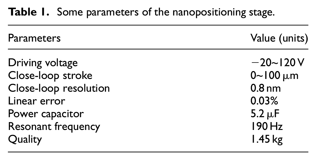
A nano-positioning experimental system is presented in Figure 1. The positioning stage (P-561.3CD) is driven by a piezoelectric actuator. Its horizontal motion range is up to 100 μm. The stage is connected to a voltage amplifier (E-727.3CDA). Displacements of the stage are measured by a built-in capacitive sensor. Based on the displacements, a host computer produces analogy voltages to drive the stage. Table 1 shows some parameters of the stage.
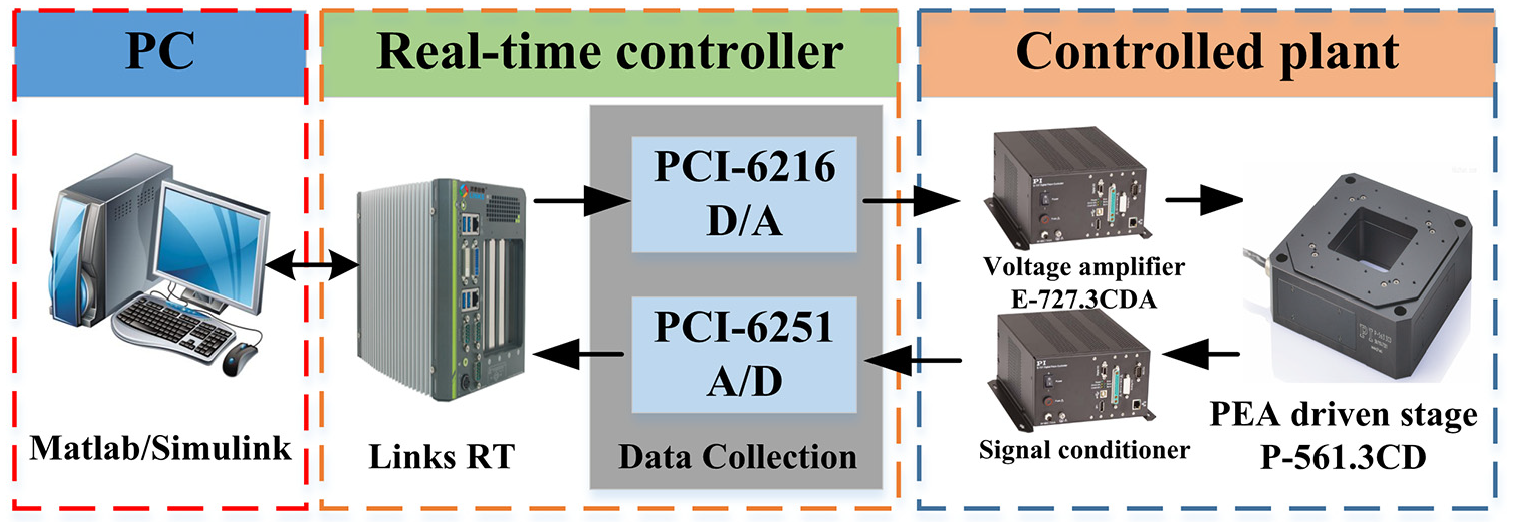
Structure of a nanopositioning system.
Some parameters of the nanopositioning stage.
Problem statements
Hysteresis, a ubiquitous nonlinear phenomenon existing in piezoelectric actuators (PEAs), seriously degrades positioning speed, accuracy, or even destabilizes a closed-loop system. Figure 2 presents hysteresis loops produced by input voltages with different frequencies. From the figure, one can see clearly that the hysteresis loops differ when input frequencies vary. Actually, it reflects the phase delays between inputs and outputs, and it challenges the precise control of a stage driven by a PEA, especially for the hysteresis model-based feedforward control, since it is difficult to get an accurate hysteresis model.
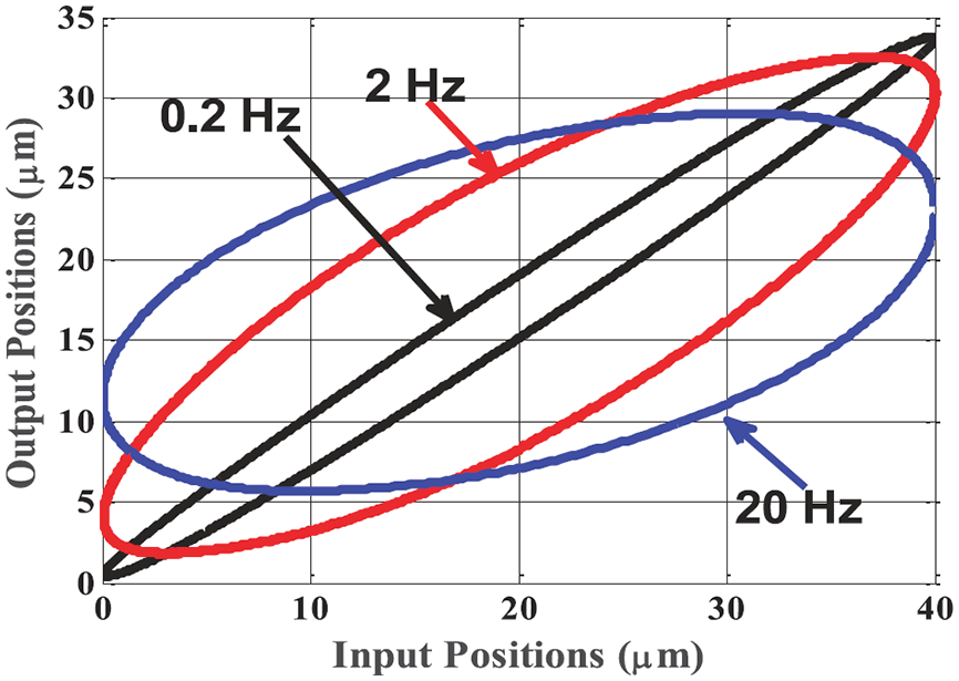
Hysteresis loops of different frequencies.
To minimize the hysteresis, an algorithm, which is independent of the hysteresis model and is able to effectively eliminate the phase delays between the inputs and the outputs, is indispensable. In next section, a UADRC is designed.
U-model based active disturbance rejection control
Brief introduction to the linear active disturbance rejection control
Active disturbance rejection control (ADRC) is a practical approach to address disturbances. An extended state observer (ESO) plays a key role in ADRC. 23 For satisfactory performance and practical design, ADRC has been applied in numerous industrial sectors.24–26
To make a brief introduction to the LADRC, considering a first-order system as follows

where y is the system output, f is the total disturbance, b0 is a control gain, and u is the control signal.
A second-order linear ESO (LESO) is
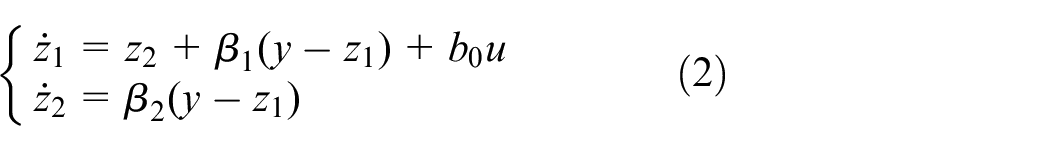
where z1 and z2 estimates
According to the bandwidth parameterization method,
27
let
Let the total disturbance estimation error be
Based on the LESO (2), a control law is designed for system (1)
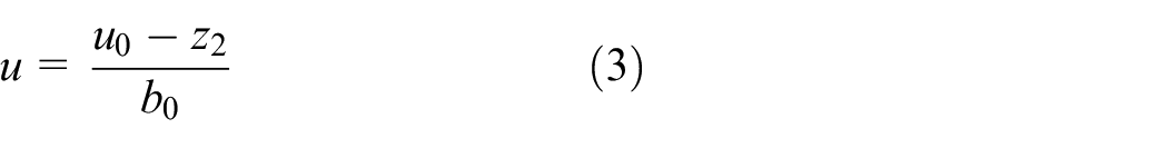
where u0 is an auxiliary control law. In the LADRC,
Substituting control law (3) into system (1), one has

Obviously, for any system, the closed-loop system is approximate to be an integrator. This is the basis of a U-model control. Next, one has to get a differential operator, then any system can be dynamically transformed to be “1.” Accordingly, the desired closed-loop dynamics can be obtained by a pre-setting control law.
The U-model based active disturbance rejection control
The UADRC design
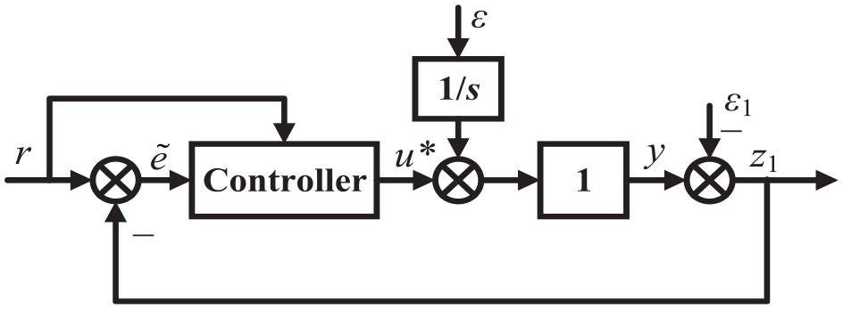
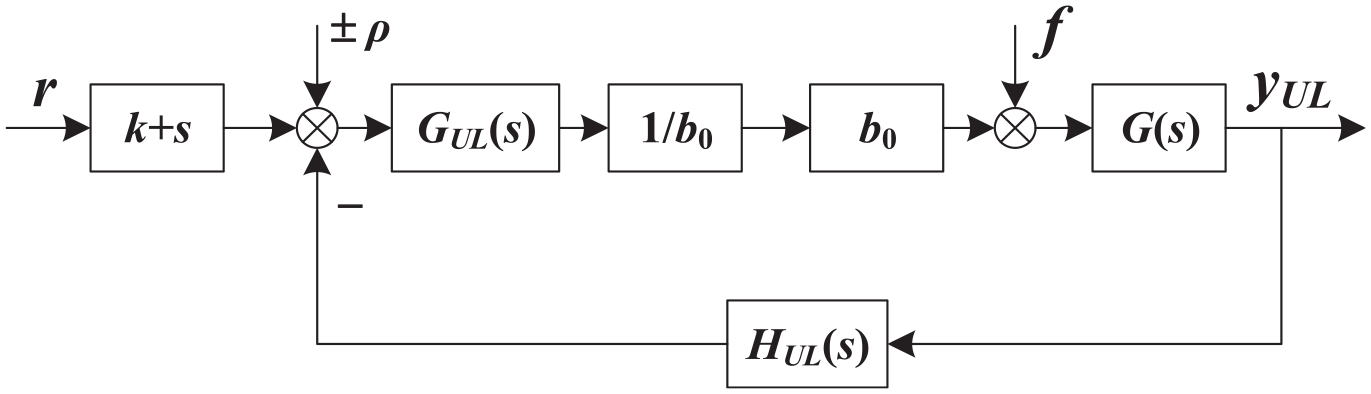
Based on above discussions, the UADRC structure can be proposed, and it is given in Figure 3.
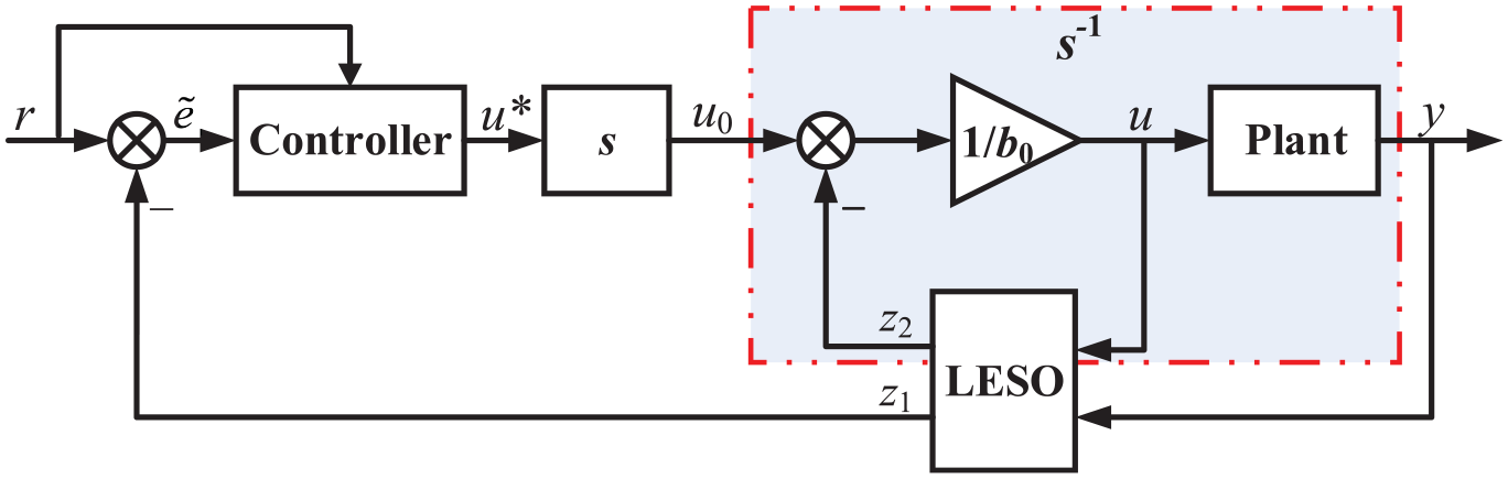
Structure of the UADRC.
Here, r is a reference,
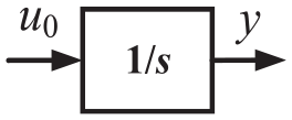
An approximate dynamics of a controlled plant.
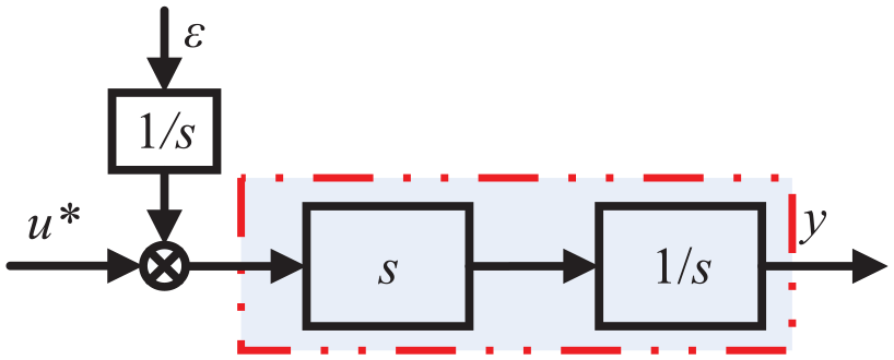
Clearly, by a LESO, a complicated plant is converted to be a simple one. However, system output y is obtained by integrating its input u0. It is known that an integration results in 90° phase lag. The phase lag reduces the response speed. If less integrators exist or even no integrator exists, less phase lag or even no phase lag will exist, and the response speed will be accelerated definitely.
Considering that Figure 4 gives out an approximate relationship between y and u0, one has (5), if the total disturbacne estimation error is defined to be ε, that is,

Accroding to key point of the UC, a differentiator is introduced (see Figure 1). Let
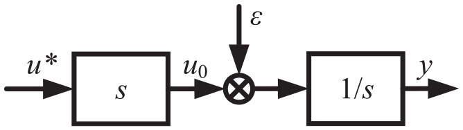
An equivalent structure of a controlled plant.
For Figure 5, its equivalent structure is shown in Figure 6.
An equivalent structure of Figure 5.
It is easy to find that, if there is no total disturbance estimation error, that is, ε = 0, for a control law
However, generally,
where
An equivalent structure of the UADRC.
then
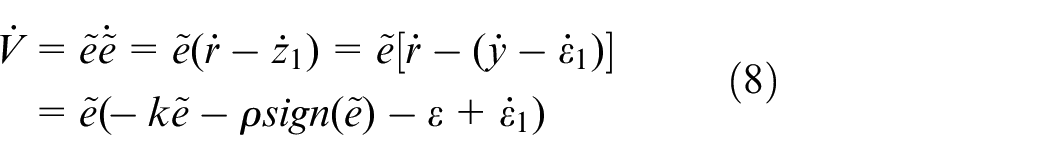
Since
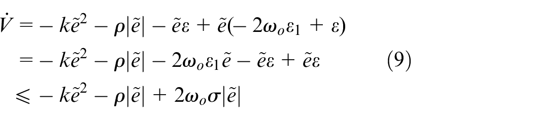
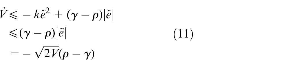
Let

Therefore, the closed-loop system is exponentially stable.
Additionally,
Define

and
In other words, control error
Steady-state tracking error
From Figure 7 and Remark 5, one has the relationship between
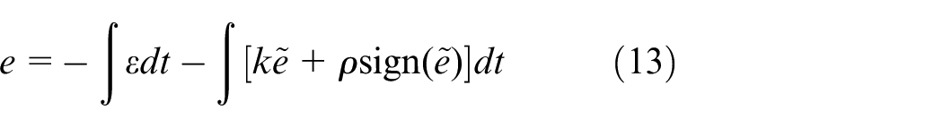
Obviously, the tracking error e is dependent on the accumulative total disturbance estimation error
According to Figure 5, one has

Substituting (6) into (14), then

that is,

Let

Define

Solution of (18) is
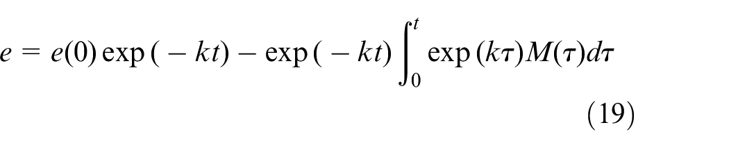
where e(0) is the initial tracking error.
Thus, steady-state tracking error ess is
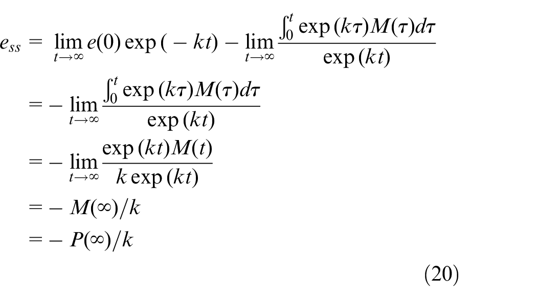
From (20), one can see that the steady-state tracking error ess is proportional to
Ensuring
A larger
A larger k ensures smaller
Here, an experience is
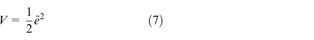
Phase analysis
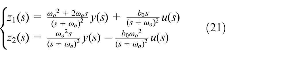
Here, for the LADRC and the UADRC, phases between the reference signal r and the system output y are compared. After taking the Laplace transformation for both sides of (2), one has
Based on (3), for LADRC, the control law is
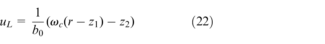
Taking (21) into consideration, one has the transfer function of
Then, an equivalent structure of the closed-loop system can be shown in Figure 8.
An equivalent structure of the closed-loop system by a second-order LADRC.
Here,
According to the superposition principle, by the LADRC, system output
Then, the frequency response is
and, phase lag of the LADRC is
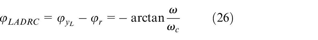
where
For
In a word, for the response of the LADRC, its amplitude is reduced, and its phase is delayed.
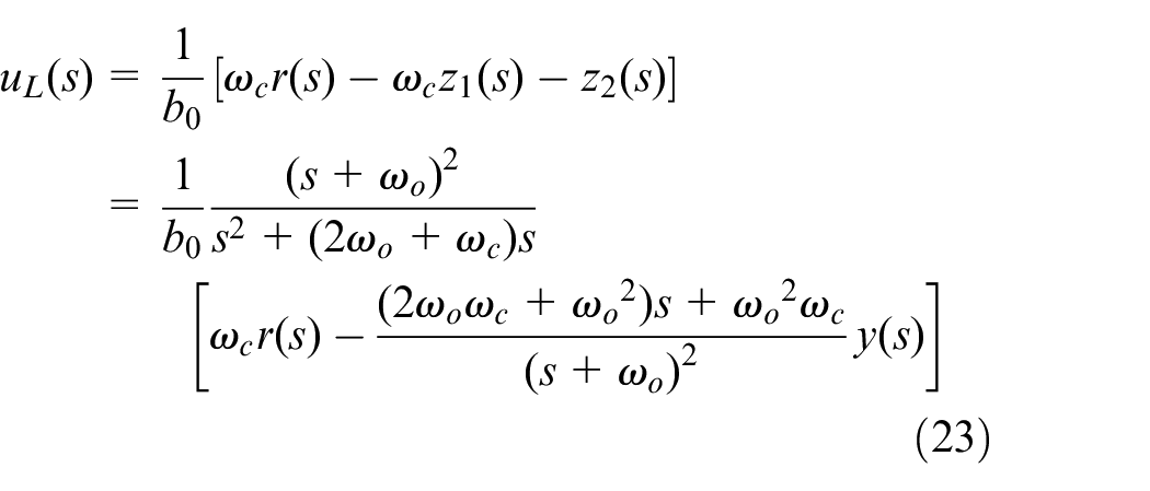
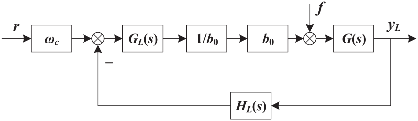
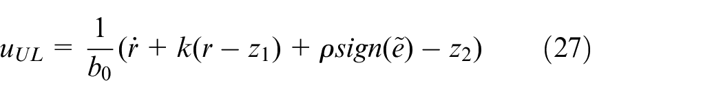
On the other hand, according to Figure 3 and (6), control law of the UADRC is
Taking the Laplace transformation for (27), one has
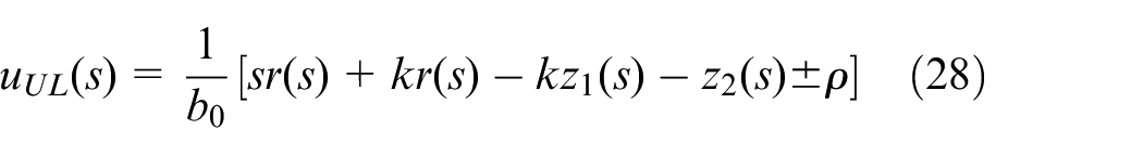
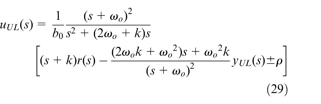
Considering (21), one has
Here,
An equivalent structure of a UADRC.
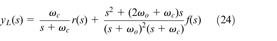
Then, system output
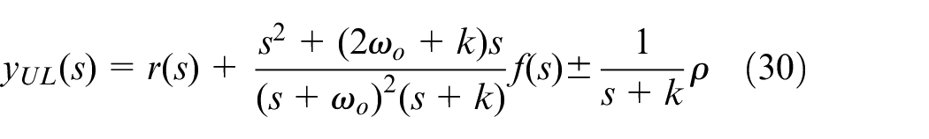
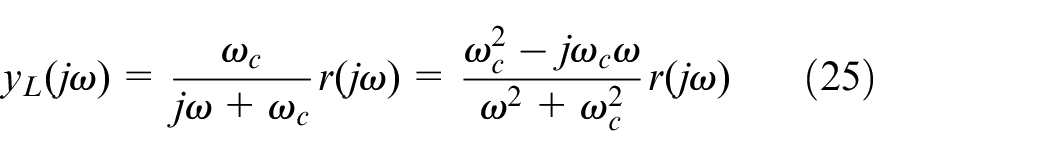
and the transfer relationship between reference r and system output

It means that, for

Obviously, no phase lag exists between

where C1, C2, and C3 are constants. Considering that
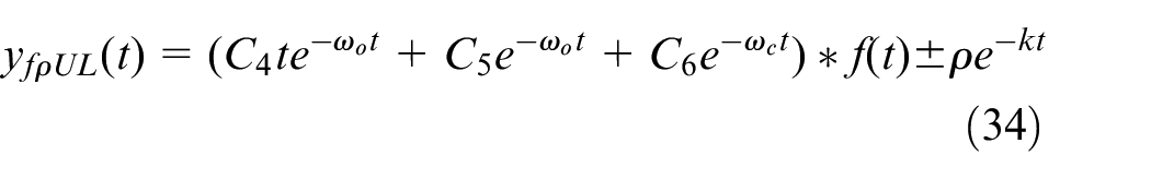
where C4, C5, and C6 are constants. It also confirms that both ρ and f will not influence the reference tracking in the steady state.
Design steps
Structure of the UADRC is given in Figure 3, tunable parameters of the UADRC are b0, k,
Step (1). The LESO (2) is designed. By choosing a suitable observer bandwidth
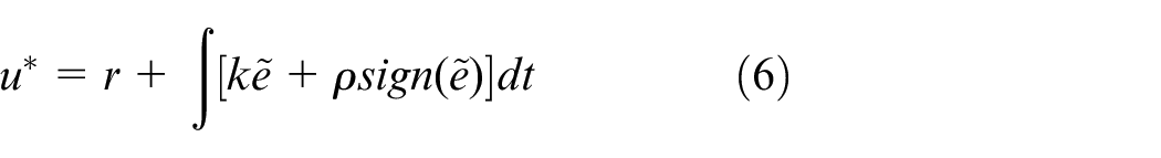
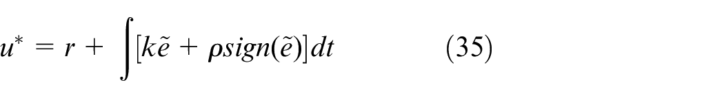
Step (2). Design u*. In this paper, u* is designed to be
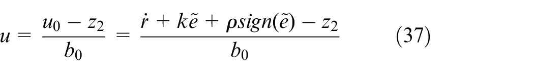
Step (3). Design u0, and it is chosen to be

Step (4). Design control law u, and it is
Then, the structure given in Figure 3 can be realized as shown in Figure 10.
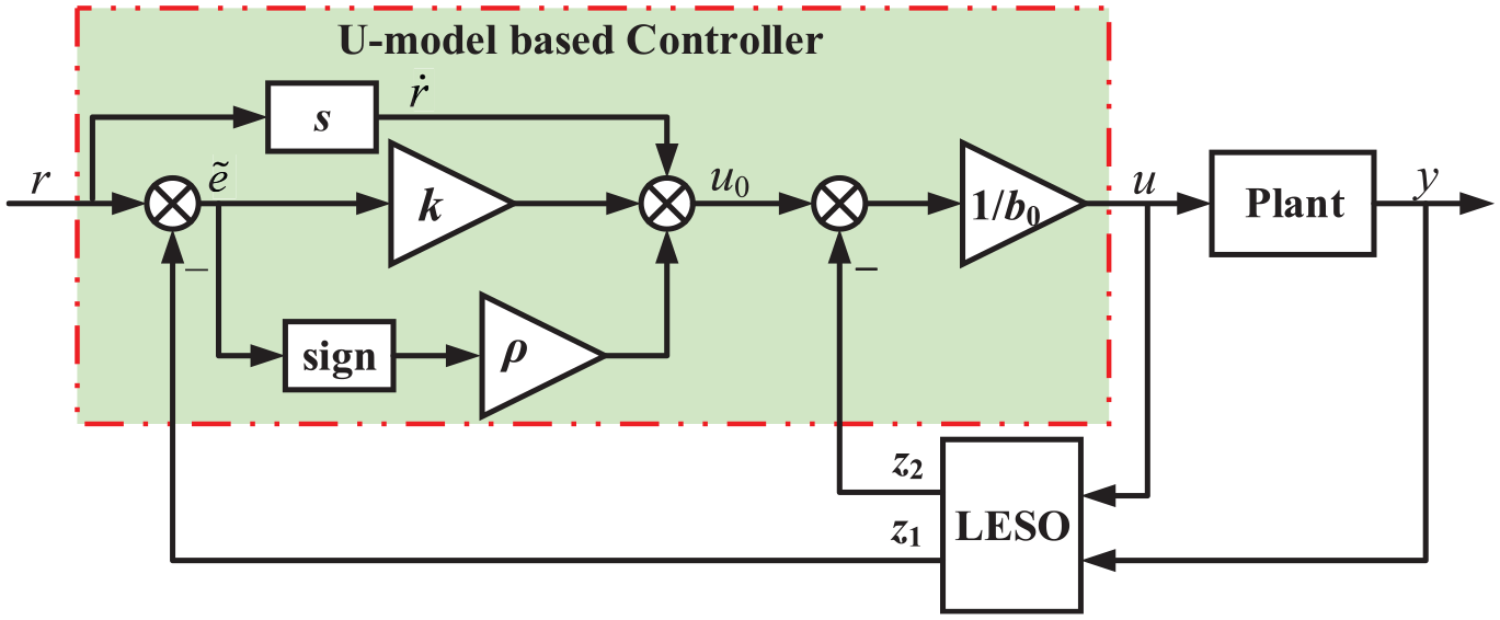
Realization of a UADRC.
Experimental results
Experiments have been performed on a commercial PEA driven stage (P-561.3CD). It is connected to a voltage amplifier (E-727.3CDA). An experimental platform is presented in Figure 11. In this work, the sampling interval is set to be 0.05 ms. To prove the UADRC, a step signal and three sine signals are set to be reference signals. Experiments with and without external disturbances have been performed. Results are given to confirm the advantages of the UADRC on both response speed and accuracy. Here, six cases are considered. Parameters of the UADRC and the LADRC are presented in Table 2.
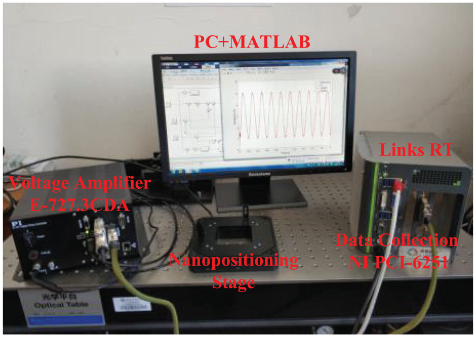
Experimental setup.
Parameters of the UADRC and the LADRC.
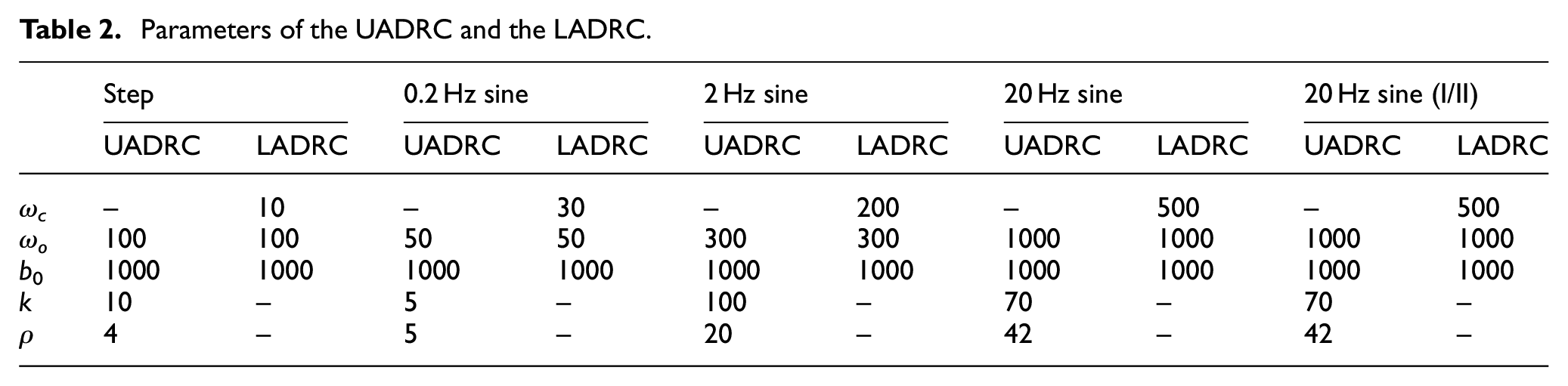
In following experiments, adjustable parameters of both UADRC and LADRC are taken form Table 2. Here, for simplification, let the case with a constant disturbance be 20 Hz Sine (I), let 20 Hz Sine (II) be the case with a sinusoidal disturbance.
Experiments without external disturbances
A step reference
Parameters of the UADRC and the LADRC are selected from Table 2. Tracking responses are given in Figure 12(a), positioning errors and control efforts are presented in Figure 12(b) and (c), respectively. It is easy to find that the UADRC has a shorter rising time. Simultaneously, by similar control efforts, tracking errors of the UADRC converges faster than those of the LADRC.
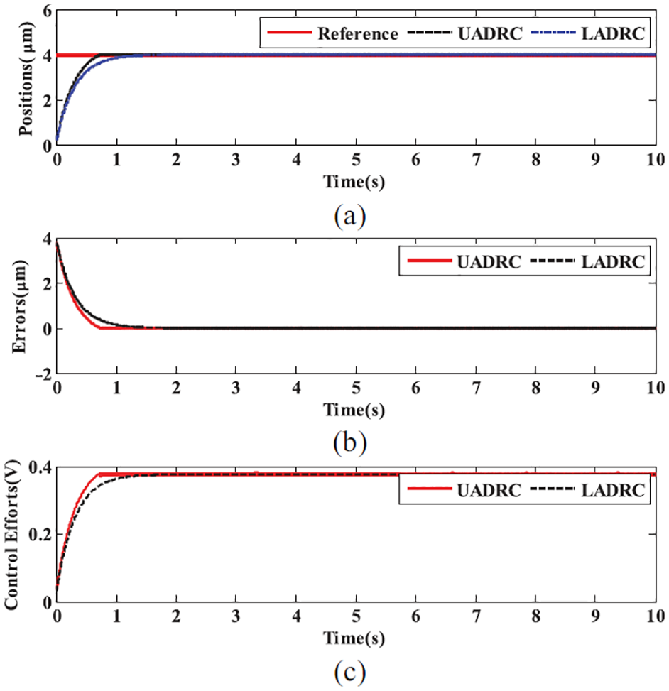
Step responses: (a) tracking results, (b) positioning errors, and (c) control efforts.
In following sections, time-varying references, that is, 0.2 Hz, 2 Hz, and 20 Hz sine signals, are considered to confirm the UADRC.
A 0.2 Hz sine reference
Let
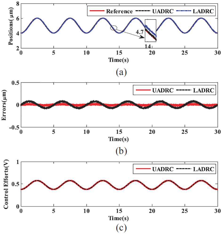
Sine responses (I): (a) tracking results, (b) positioning errors, and (c) control efforts.
Obviously, for a 0.2 Hz sine reference, both LADRC and UADRC can achieve desired responses. However, by similar control energy, the UADRC has much smaller tracking errors. Additionally, Figure 13(a) shows distinct phase advantage of the UADRC.
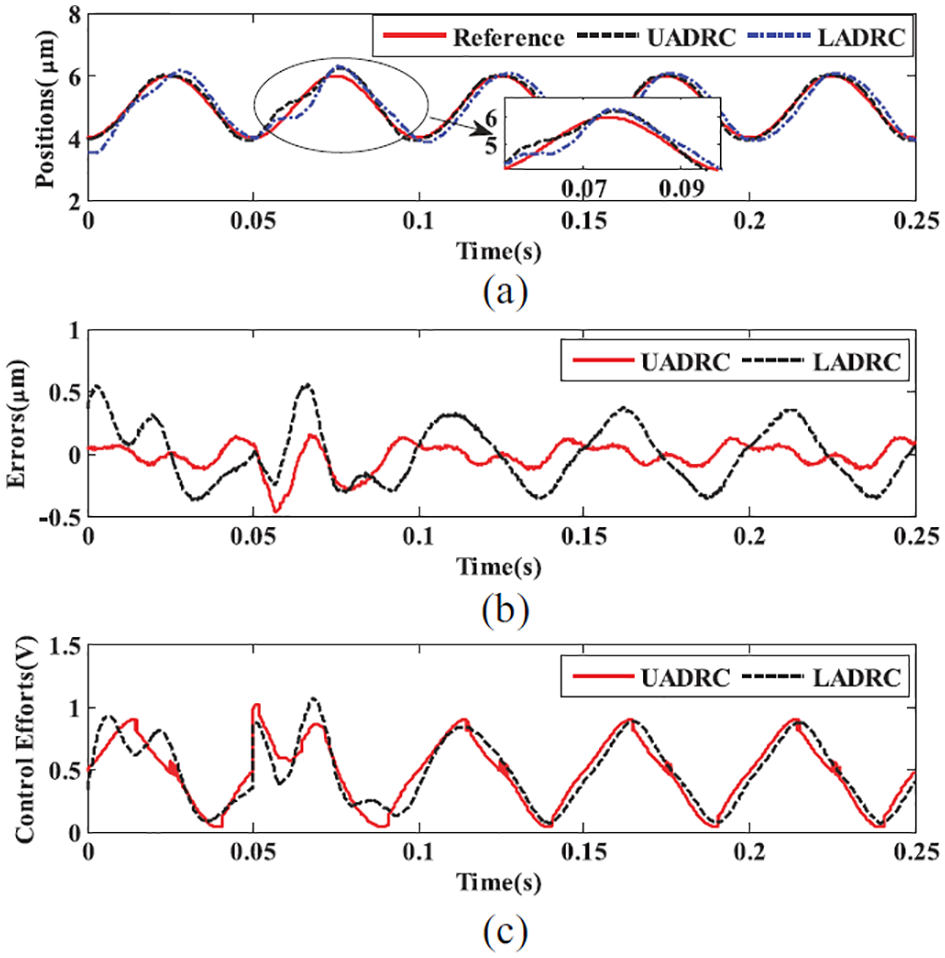
A 2 Hz sine reference
A sinusoidal signal
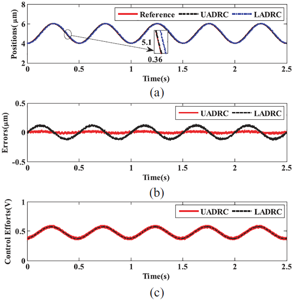
Sine responses (II): (a) tracking results, (b) positioning errors, and (c) control efforts.
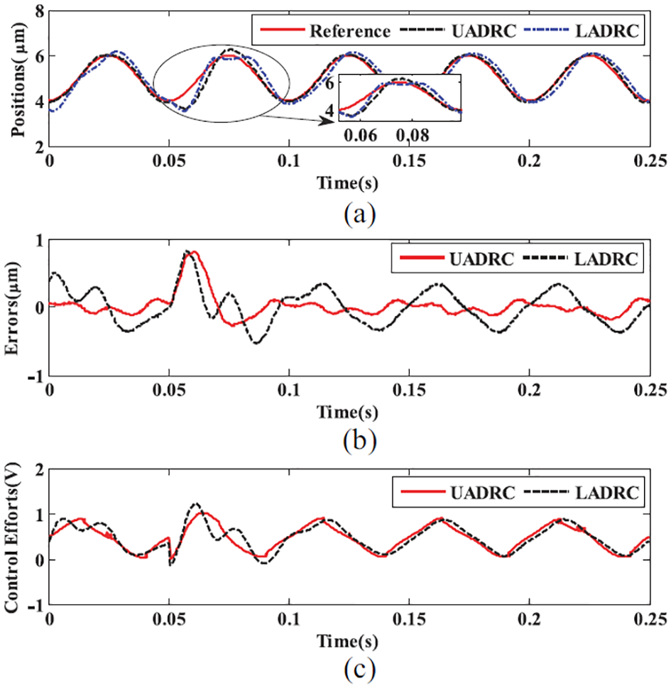
A 20 Hz sine reference
Let
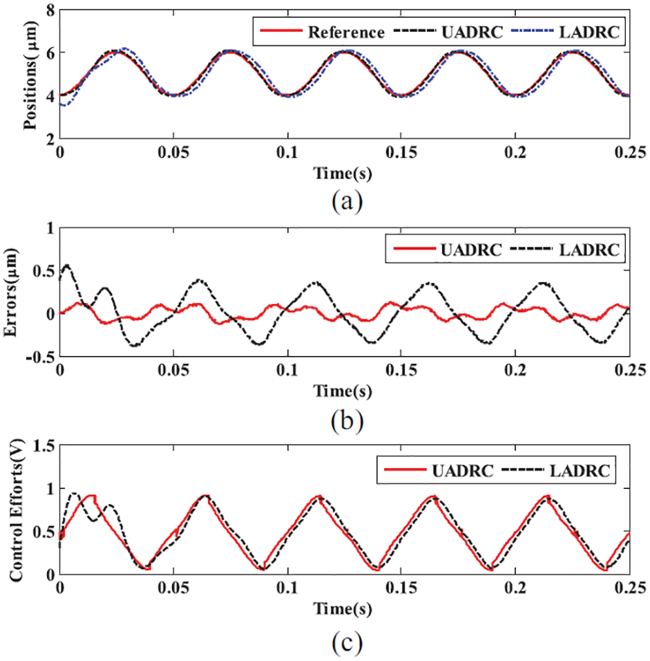
Sine responses (III): (a) tracking results, (b) positioning errors, and (c) control efforts.
Simultaneously, hysteresis is a key matter in reducing the positioning accuracy. Figure 16 shows the compensated hysteresis loops, when frequencies of the references are 0.2 Hz, 2 Hz, and 20 Hz, respectively. An ideal case is that the hysteresis loop becomes a 45° line after compensation. A smaller hysteresis loop signifies a better compensation. Obviously, in all cases, the UADRC behaves best.
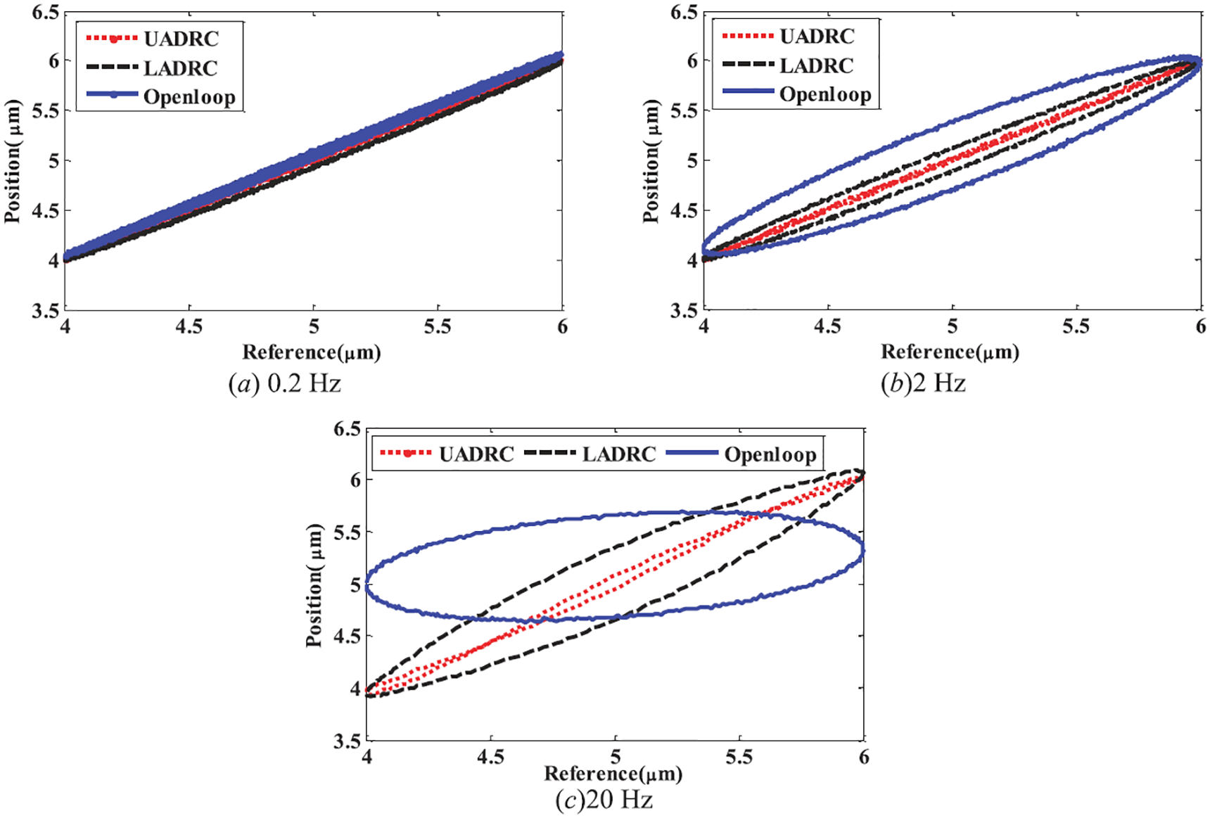
Hysteresis in a piezoelectric actuator: (a) 0.2 Hz, (b) 2 Hz, and (c) 20 Hz.
Experiments with external disturbances
In this section, external disturbances are introduced to verify the disturbance rejection ability of both UADRC and LADRC. Let
Sine responses (IV): (a) tracking results, (b) positioning errors, and (c) control efforts.
Sine responses (V): (a) tracking results, (b) positioning errors, and (c) control efforts.
From Figures 17 and 18, one can see clearly that the LADRC is weak to track a 20 Hz sine reference. However, the UADRC is still able to track the sine reference well, even if there exist a constant and a time-varying disturbance.
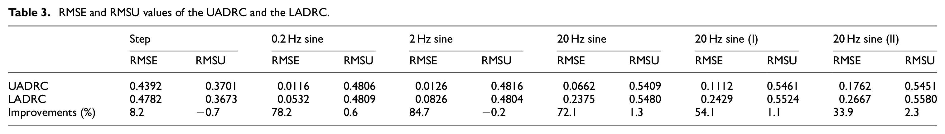
To make a quantitative comparison, values of root mean square error (RMSE) and root mean square error of control signal u (RMSU) are listed in Table 3. Here, improvements in Table 3 means the difference between the UADRC and the LADRC. If the value of the UADRC is smaller than the one of the LADRC, the improvement will be positive. Otherwise, the improvement will be negative. From Table 3, it is easy to get a conclusion that, compared with the LADRC, the UADRC has much smaller RMSE values with similar RMSU values. Additionally, when a constant disturbance and a sinusoidal disturbance exist, much better reference tracking can be also obtained by the UADRC with similar control energy.
RMSE and RMSU values of the UADRC and the LADRC.
With an attempt to show the fact vividly, histograms of both RMSE values and RMSU values are drawn in Figure 19. It also confirms that, with similar control energy, the UADRC tracks the references more accurately.
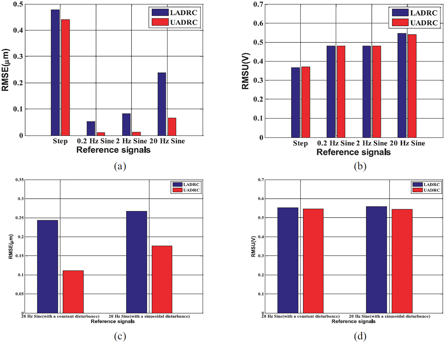
RMS values of the LADRC and the UADRC, (a) RMSEs, (b) RMSUs, (c) RMSE of the 20Hz Sine (with external disturbances), and (d) RMSU of the 20Hz Sine (with external disturbances).
Obviously, tracking errors shown in figures, RMSE values given in Table 3 and Figure 19 reveal a fact that the U-model based control law u* proposed in the UADRC is capable of achieving much faster and more accurate responses no matter whether external disturbances exist or not. Moreover, the PD control law in the LADRC is not able to drive the system output track references as desirably as u*. Phase advantage of the UADRC is more remarkable in the case of tracking a higher frequency reference. Finally, it is worth pointing out that more satisfactory tracking responses can be obtained by similar control energy.
Conclusion
In this paper, by integrating advantages of both active disturbance rejection control and U-model control, a U-model based active disturbance rejection control is proposed and it is verified on a piezoelectric driven nano-positioning stage. Phase advantage of the UADRC is confirmed by both theoretical and experimental results. Better tracking performance is produced in a practical way. Therefore, the UADRC may be a promising way in the positioning control. Additionally, from theoretical analysis of the steady-state tracking error, one can also find that a better ESO and a more powerful control law ensure much smaller tracking errors. As a continuous research, a more effective ESO and a more robust control law in the UADRC promise much better closed-loop performance, and it is on the way.
Footnotes
Acknowledgements
The authors are grateful to the editors and the anonymous reviewers for their helpful comments and constructive suggestions with regard to the revision of the paper.
Declaration of conflicting interests
The author(s) declared no potential conflicts of interest with respect to the research, authorship, and/or publication of this article.
Funding
The author(s) disclosed receipt of the following financial support for the research, authorship, and/or publication of this article: This work is supported by National Natural Science Foundation of China (61873005, 61403006), and Key program of Beijing Municipal Education Commission (KZ201810011012).