
Abstract
In this paper, the dynamics and control strategies of a biped robot with 6-DOF parallel leg mechanism are studied. Firstly, the multi-body kinematic model and dynamic model of the robot are established. Secondly, the insufficient stiffness of robot’s feet and the coupling effect between the kinematic chains are considered in dynamics modeling, and the rigid-flexible coupling model is established by using ADAMS and finite element method. Finally, aiming at the position deviation and system vibration caused by the flexible foot, a strategy based on the combination of a computed torque controller (CTC) and a second-order sliding-mode super twisting algorithm (STA) is designed. At the same time, the control strategy based on CTC and PID and the control strategy based on CTC and sliding mode control (SMC) are designed to compare with CTC-STA. The results show that CTC-STA has faster regulation ability and stronger robustness than CTC-SMC and CTC-PID.
Introduction
Mobile robots are more and more widely used in many fields and the analysis of function and stability is essential in robot research and application.1,2 At present, the legs of most mobile robots are connected in series by a group of open-loop kinematic chains, which have the characteristics of large-scale workspace, poor stiffness, and simple dynamics.3–5 In order to enhance the load-carrying capacity and stiffness, more and more robots with parallel leg mechanism are being developed and studied.6–8 In theory, since the load is supported by multiple chains, parallel leg mechanism tends to have a large load-carrying capacity and high structural stiffness. 9 However, this kind of leg mechanism has complex dynamics and control algorithm problems10,11 as well as difficult forward kinematics. 12
The kinematic model can reflect the mapping relationship between joint motion and spatial motion of the mechanism without considering the effect of force, while the dynamic model is to study the relationship between mechanical motion and force.13,14 In the dynamic model, using CTC as dynamic compensation can make the robot become a more easily controlled system. Zhang et al. 15 designed an adaptive robust decoupling controller based on time-delay estimation (TDE) and sliding mode control (SMC) for a multi-arm space robot. The dynamic coupling of the robot was compensated by TDE technology, then SMC complemented and reinforced the robustness of the TED. Van et al. 16 proposed a new method based on the combination of CTC, high-order SMC and fuzzy compensator to control uncertain robot manipulators by using only position measurements. A third-order SMC observer was used to observe the speed and identify the uncertainty, and fuzzy compensator was proposed to enhance capability of the tracking performance.
The flexible joints and components have great influence on the kinematic and dynamic performance of the robot, and the uncertain factors not considered in the model will be enlarged. Slender rods and joints in robot structures are generally considered to be flexible.17,18 Yang et al. 17 established the rigid-flexible coupling model of a 6-DOF Stewart platform with flexible joints in ADAMS and MATLAB, and the explicit dynamic equations are established based on the pseudo-rigid-body model and the principle of virtual power. Elghoul 19 proposed a fault-tolerant control method of a flexible joint robot to compensate for the lost performance due to the uncertainty. The singular perturbation method was used to reduce the dynamic model of the flexible joint robot in a fast and slow subsystem.
In this paper, a biped robot with 6-DOF parallel leg mechanism is studied. The insufficient stiffness of the foot structure in space leads to large trajectory deviation and even vibration, and the coupling effect between the kinematic chains is strengthened. In order to improve the dynamic performance and the robustness of the control system, a strategy based on the combination of CTC and STA is designed to adjust the system uncertainty caused by the flexible foot. CTC-PID and CTC-SMC strategies are designed for comparison. The contribution of this paper is to provide a dynamic analysis method of the flexible parts of the robot system, and then take the flexible deformation into account in the dynamic control, and provide a feasible control strategy.
Robot structure and dynamics modeling
Robot structure
The schematic diagram of the robot prototype and the kinematic chain are shown in Figures 1 and 2, respectively. Each leg has six kinematic chains (
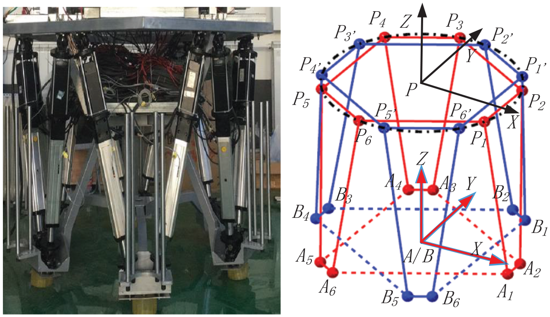
Robot structure diagram.
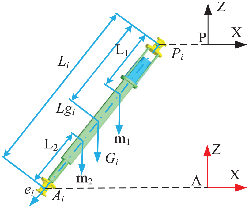
Kinematic chain diagram.
In order to simplify the robot model and facilitate the analysis, the following provisions are made:
The center of mass (COM) of the upper platform (P) is located in the center of all the joints (
The friction and clearance in the system can be ignored;
The motion process of foot A relative to P is taken as the research object.
As shown in Figure 1, the upper platform coordinate is defined as {P: O-XYZ}, and the two foot coordinate systems are {A: O-XYZ} and {B: O-XYZ}, respectively. In the initial configuration, coordinate system {A} and {B} are coincident. In Figure 2,
Kinematic model
The robot’s motion is realized by changing the relative position among the coordinate systems {P}, {A}, and {B}. It is stipulated that

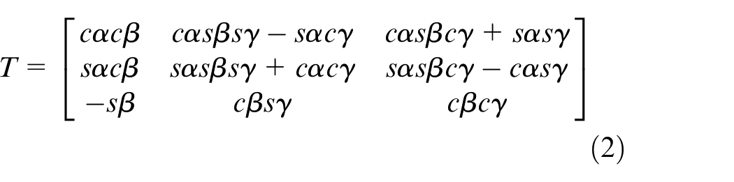
where T is the rotation matrix,
where

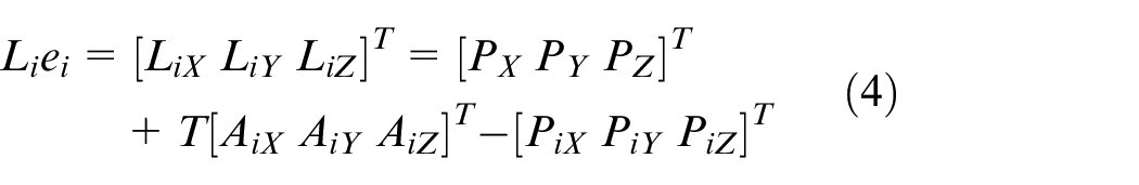
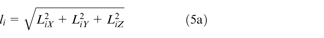
It can be obtained that the vector
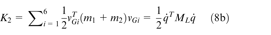
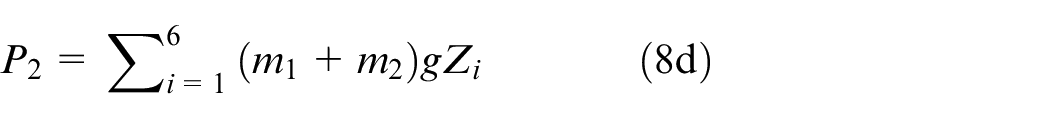
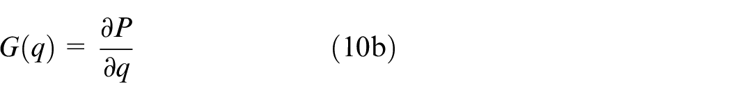
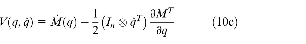
Dynamic model
where

where

where

where

where

where
Flexible component analysis
As shown in Figure 1, the stiffness of foot A in space is not high, which easily leads to large position deviation and even system vibration in the process of robot motion. In order to calculate the influence of elastic deformation on the large-scale movement of foot A, a hybrid coordinate is proposed to describe the displacement.

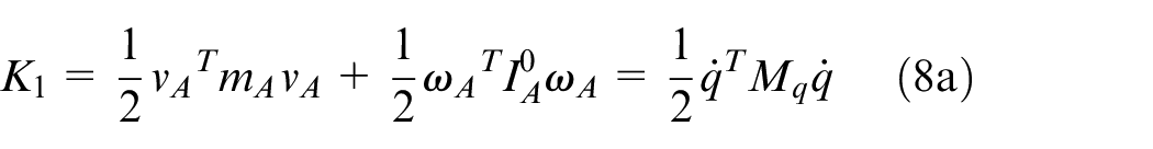
The kinetic energy equation
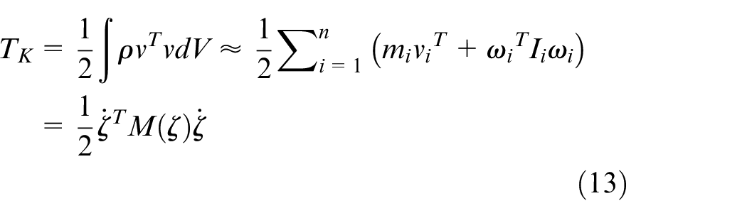
where
The potential energy equation U of the flexible body can be calculated as equation (14):
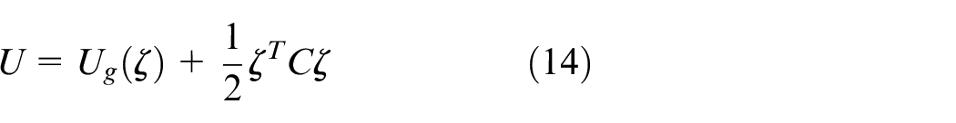
where C is the stiffness matrix;
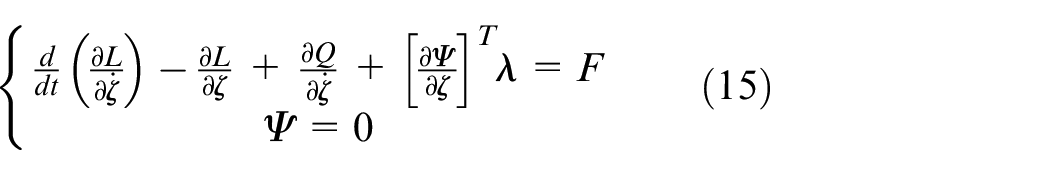
where
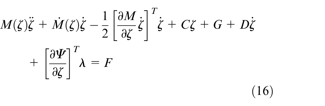
where
where
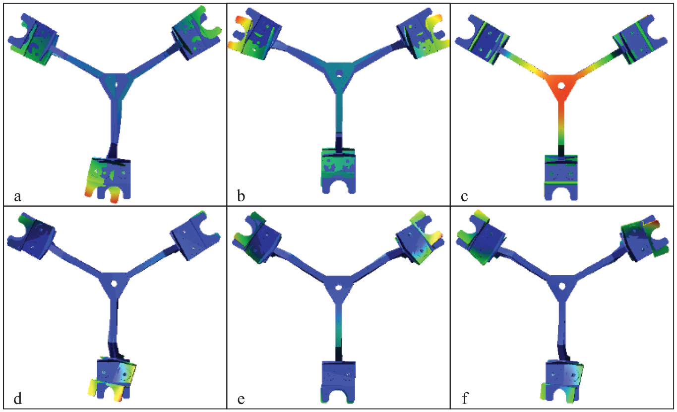
Deformation of foot A.
The rigid-flexible coupling model in ADAMS is shown in Figure 4.
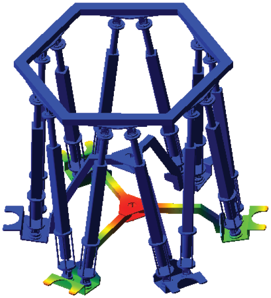
Rigid-flexible coupling model of leg A in ADAMS.
The X-axis is selected as the forward direction of the robot, and the trajectory is planned according to equation (18a):

The speed and acceleration of the swinging leg at the beginning (t = 0 s) and the end (t = 1.5 s) are both 0, the single step distance is 0.2 m.
According to equations 18(a) and 5(a), the displacement of each kinematic chain can be obtained. Figure 5(a) depicts the movement of foot A in the case of rigidity and flexibility as it moves according to trajectory equation (18). P1, V1, and A1 respectively represent the displacement, velocity and acceleration when foot A is a rigid body, P2, V2, and A2 respectively represent the displacement, velocity and acceleration when foot A is flexible, e1, e2, and e3 are position error, velocity error and acceleration error between flexible model and rigid model, respectively. In Figure 5(b), Ji and J’i represent the main force of
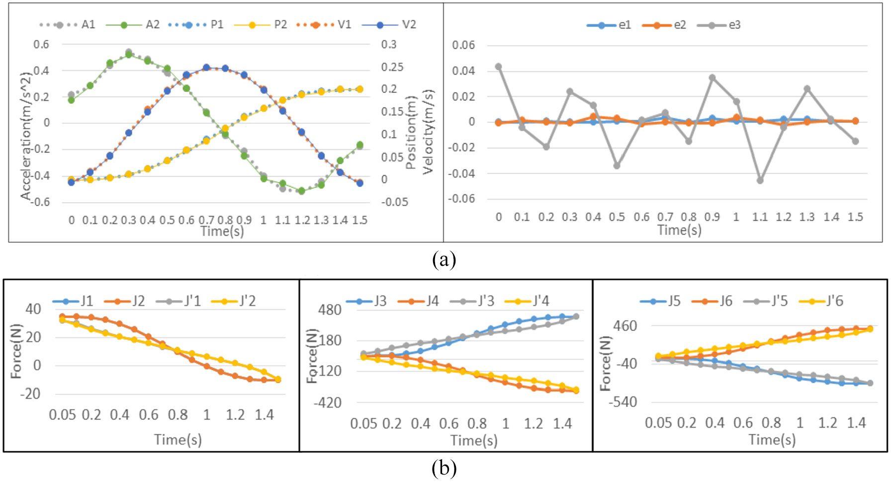
Movement of foot A: (a) movement in X direction and (b) joint force.
Figure 5 shows that foot A can track the planned trajectory whether it is flexible or rigid. Compared with the rigid body, when foot A is a flexible body, the acceleration jitters and changes in a large range. In order to obtain reliable simulation results, the effect of foot A’s deformation is treated as position disturbance, as shown in equation 18(b):
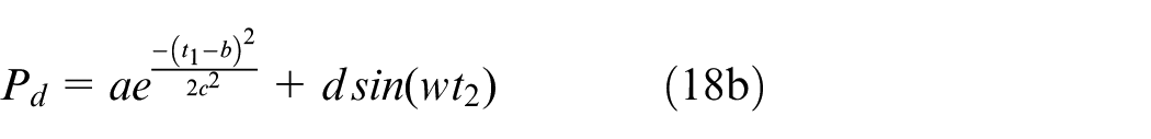
where the first term is Gauss function, which represents the position change caused by rebound deformation when foot A leaves the ground; the second term is trigonometric function, which represents the swing caused by the coupling action from foot A’s flexibility.
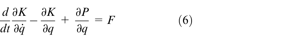
Dynamic decoupling and control
CTC-based PID
The calculated torque controller (CTC) is widely used in the controller design of industrial robot and manipulator.
15
An internal control loop is introduced into the dynamic control of the robot, whose function is to dynamically compensate the system. As shown in Figure 6, the traditional CTC combines the calculation of nonlinear force term
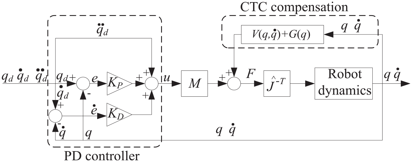
CTC-based PD decoupling strategy.
The CTC law can be expressed as:


where


Equation (20) can be expressed in the form of state space:

where

It is obvious that by choosing
CTC-based STA
When the system model is accurate enough, the CTC-PD control strategy can achieve good effect by selecting
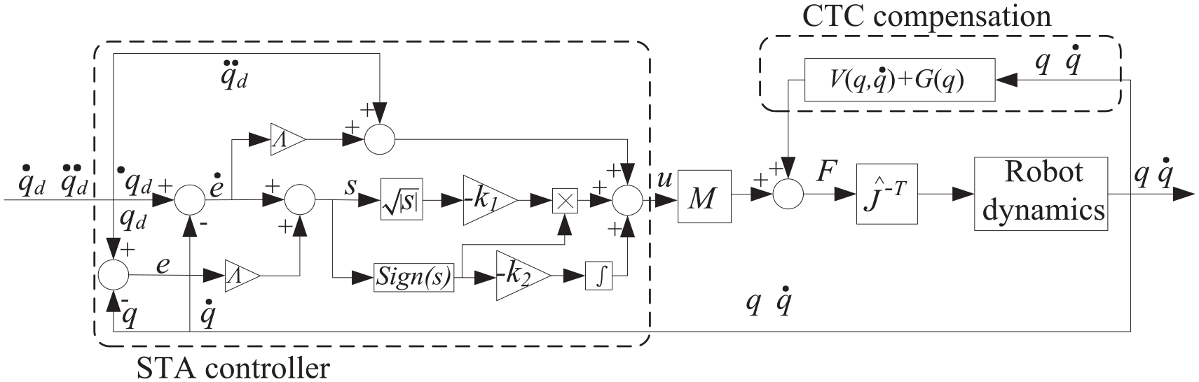
CTC-based STA decoupling strategy.
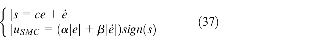
STA sliding surface vector is designed as equation (23):

where Λ>0

where

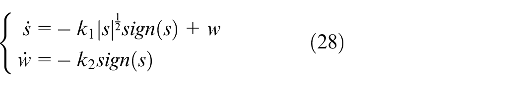
The sliding mode control (SMC) can be expressed by equation (26):

where
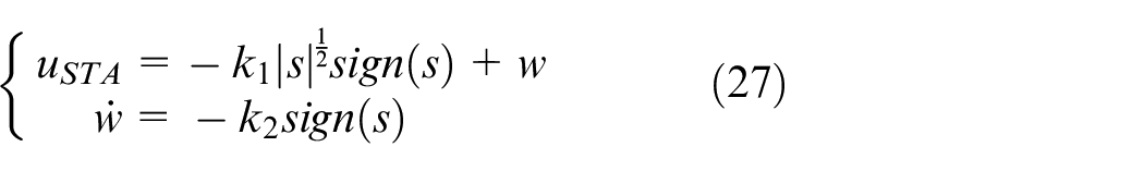
where
From equations (25), (26), and (27), equation (28) can be obtained:
The closed-loop system’s stability can be proven by Lyapunov function:

where

where
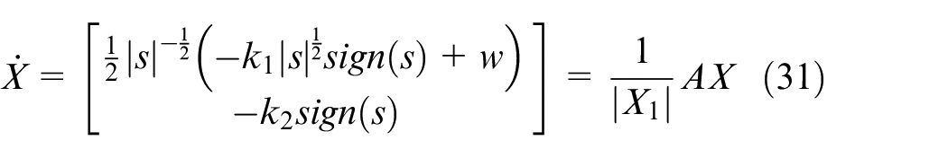
The derivative of equation (29) with respect to time is shown as equation (32).
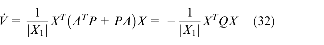
According to equation (29), equation (33) can be obtained:

where
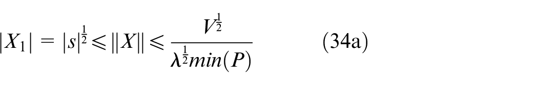
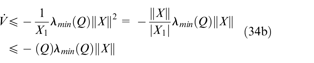
Equation (35) can be obtained from equation (33):
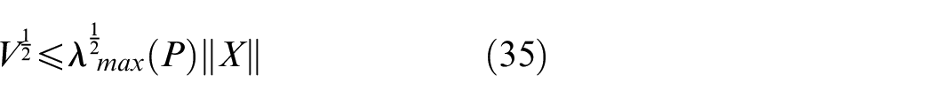
Substituting equation (34) into equation (35) yields:
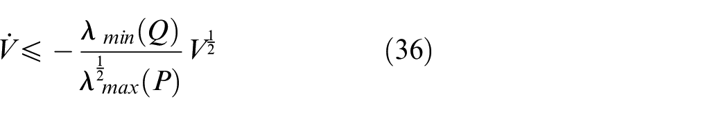
It can be obtained that the closed-loop system equation (28) tends to 0 in finite time, and
Numerical simulation and analysis
In this section, in order to verify the influence of flexible parts on the system and the performance of CTC- based PID and CTC-based STA, the simulation model is built in Matlab/Simulink and ADAMS / flex, as shown in Figure 8. When leg A moves as equation 18(a), the driving force
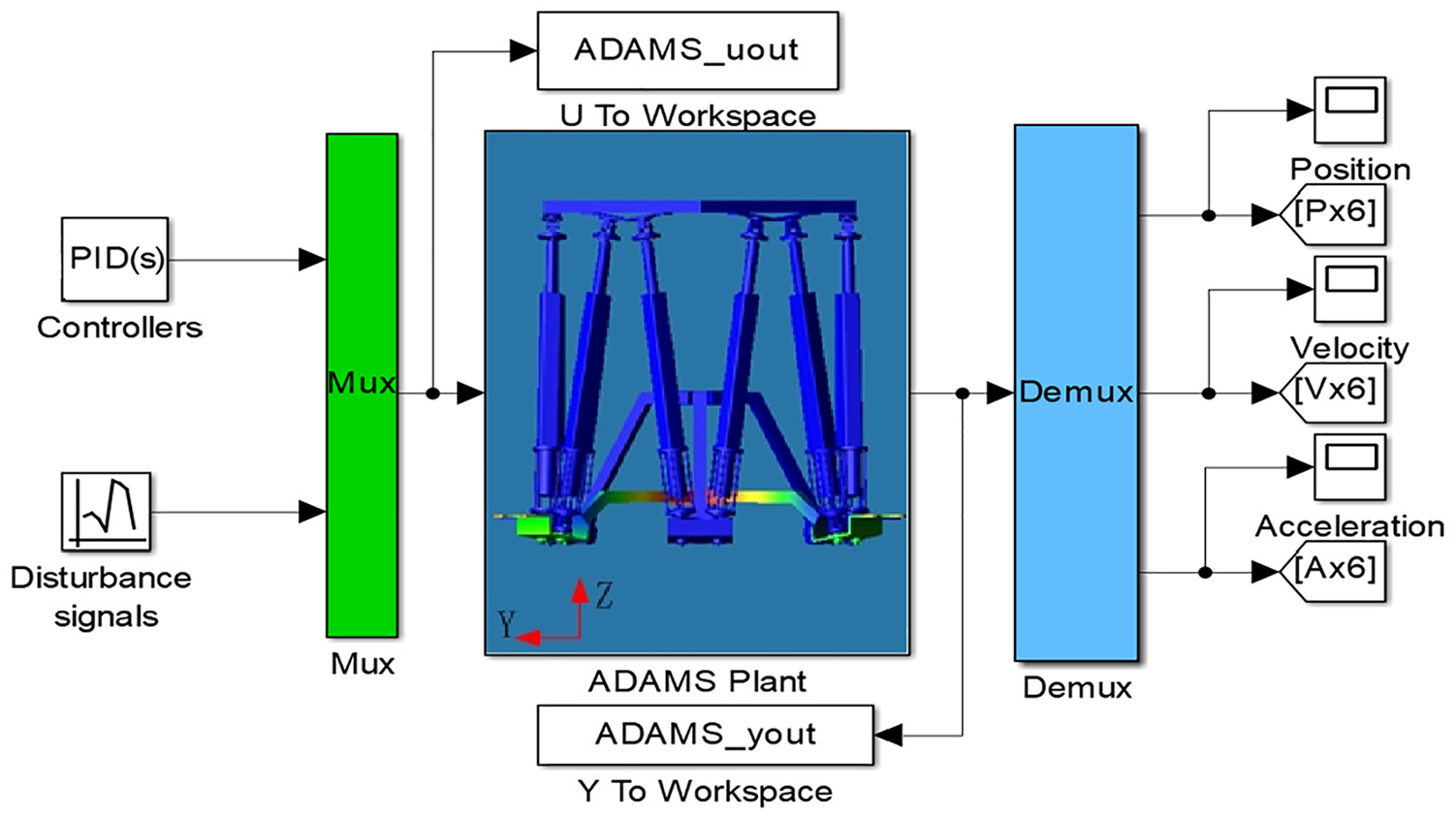
Rigid-flexible coupling model of robot.
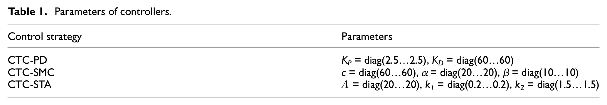
Parameters of controllers.
The simulation work is divided into two parts. The first part is to compare the effects of CTC-PD, CTC-SMC, and CTC-STA on the nominal model, and obtain the trajectory tracking performance of foot A. In the second part, the performance of the three methods are compared in the case that foot A is flexible.
The performance of the controllers to the nominal model is shown in Figure 9, where IT represents the ideal trajectory, CT represents the common PID control, ST represents the STA control, CST represents the common SMC control; CE, SE and CSE are the errors between CTC-PID, CTC-STA, CTC-SMC and the ideal trajectory respectively. In Figure 9(b), CF is the resultant force of Ai (i = 1..6) in Z direction with CTC-PID control, SF is the resultant force of Ai in Z direction with STA control.
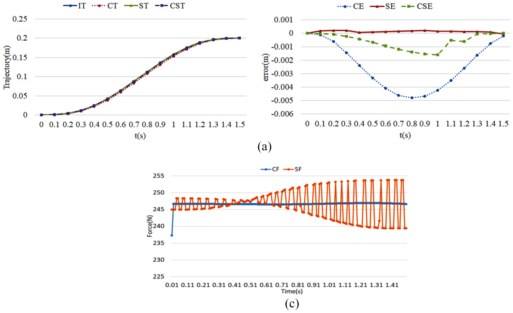
Nominal model control: (a) Trajectory tracking curve and error and (b) Resultant force in Z direction.
The simulation results show that all the three kinds of controllers can make the nominal model track the ideal trajectory accurately. Compared with CTC-STA, the tracking errors of CTC- PID and CTC-SMC method are larger. From Figure 9(b), it can be seen that when leg A moves as equation (18), the Ai’s resultant force in Z direction is used to offset the gravity of foot A. And due to the sliding surface, the resultant force presents buffeting.
In accordance to the analysis in Section 2.4, simplify the effect of foot A’s flexibility and apply it to {A} as equation (18b) when foot A is considered as a flexible part. The performance of the three controllers is shown in Figure 10, FCT, FST and FCST are the trajectories of CTC-PD, CTC-STA, and CTC-SMC, respectively.
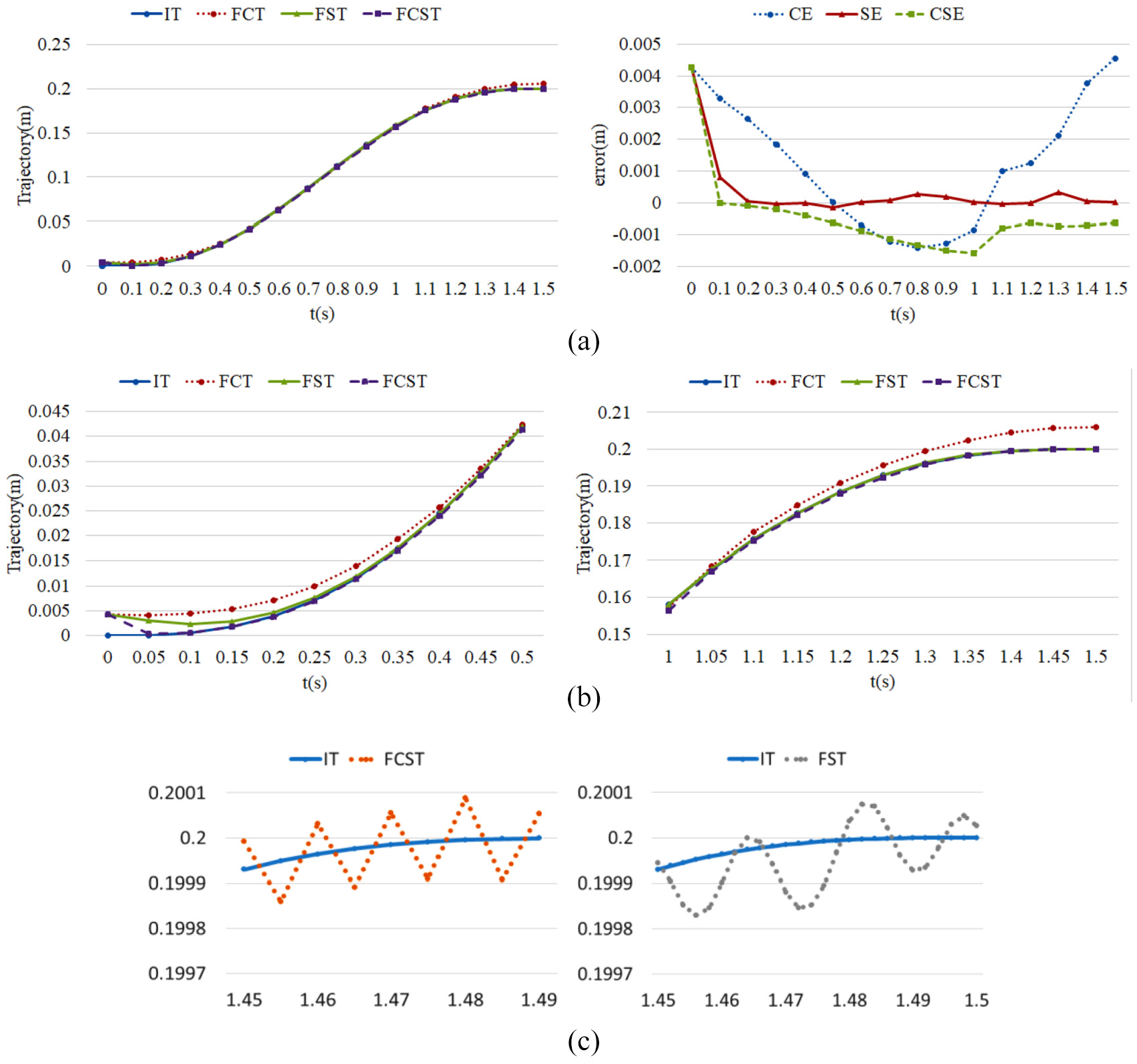
Tracking performance: (a) Trajectory tracking curve and error, (b) Enlarged view of the trajectory tracking, and (c) CTC-SMC and CTC-STA.
It can be seen from Figure 10(a) and (b) that although the position of foot A is greatly deviated due to rebound motion in the early stage (0–0.5 s), all the three controllers can quickly adjust the position to make foot A accurately track the ideal trajectory, and CTC-STA and CTC-SMC show better adjustment performance than CTC-PD. When foot A vibrates (1–1.5 s), the trajectory tracking error of CTC-PD increases gradually. CTC-STA and CTC-SMC still have strong adjustment ability, which makes the trajectory close to the ideal trajectory, and CTC-STA has the best tracking performance. Common SMC has properties such as robustness, parameter variations, reduced order dynamics, while STA retains most of the properties and its higher order derivative is activated on the sliding variable instead of first derivative. As shown in Figure 10, the output of CTC-STA controller is continuous and gentle, which is beneficial to the system.
Conclusion
In this paper, a super twisting sliding mode controller based on computational torque control is proposed for the control of a heavy-duty walking robot with flexible structure, the PID control based on CTC and the SMC control based on CTC are designed for comparison. CTC- PID, CTC-SMC and CTC-based STA are model-based decoupling control strategies, but CTC- PID is more dependent on the model accuracy. When there are flexible components or large model errors and external interference in the system, the CTC-PID maybe not able to achieve satisfactory performance. By introducing the STA strategy, the trajectory can be accurately tracked, which can effectively reduce the coupling effect and improve the robot’s performance and robustness. The combination of CTC and STA improves the potential of robot dynamics in practical application.
Footnotes
Declaration of conflicting interests
The author(s) declared no potential conflicts of interest with respect to the research, authorship, and/or publication of this article.
Funding
The author(s) received no financial support for the research, authorship, and/or publication of this article.