Improved artificial immune algorithm for the flexible job shop problem with transportation time

Abstract

The flexible job shop problem (FJSP), as one branch of the job shop scheduling, has been studied during recent years. However, several realistic constraints including the transportation time between machines and energy consumptions are generally ignored. To fill this gap, this study investigated a FJSP considering energy consumption and transportation time constraints. A sequence-based mixed integer linear programming (MILP) model based on the problem is established, and the weighted sum of maximum completion time and energy consumption is optimized. Then, we present a combinational meta-heuristic algorithm based on a simulated annealing (SA) algorithm and an artificial immune algorithm (AIA) for this problem. In the proposed algorithm, the AIA with an information entropy strategy is utilized for global optimization. In addition, the SA algorithm is embedded to enhance the local search abilities. Eventually, the Taguchi method is used to evaluate various parameters. Computational comparison with the other meta-heuristic algorithms shows that the improved artificial immune algorithm (IAIA) is more efficient for solving FJSP with different problem scales.

Introduction

In recent years, increasing numbers of enterprises have been paying more attention to the problem of how to optimize the scheduling of workshop to maximize their efficiency. As a result, the job-shop problem (JSP) has become one of most popular research topics in the literature owing to its potential to dramatically decrease costs and increase throughput. This has created a need for research on the scheduling problem. Traditional JSP can be concluded as follows: there are a set of jobs to be carried out on a set of machines, where each job involves multiple operations and each operation can be carried out by only one machine. In addition, each machine can process only one job at a time. However, the canonical JSP is restricted by factors related to having a rigid model, while flexible job shop scheduling resembles actual job shop circumstances more accurately. ¹ Compared to the traditional JSP, the flexible job shop problem (FJSP) is a practically useful extension of the JSP in which each operation should be assigned to a set of alternative machines, with the result that the FJSP is much more complicated than the traditional JSP. ² Because the JSP is strongly NP-hard, the FJSP is strongly NP-hard as well. ³

In view of the fact that FJSP can effectively improve the production efficiency of the job shop and shorten the manufacturing time, multiple heuristic or meta-heuristic algorithms have been developed to optimize the problem. For example, Pezzella et al. ⁴ introduced a genetic algorithm (GA) framework integrating different strategies for developing efficient algorithms for the problem effectively. Girish and Jawahar ⁵ described a powerful particle swarm optimization (PSO)-based heuristic algorithm for FJSP to minimize the makespan. Li et al. ⁶ proposed a novel tabu search (TS) algorithm by combining an effective neighborhood structure and local search methods based on the critical block theory. Aiming for flexible job shop scheduling with the constraint of preventive maintenance activity, Gao et al. ⁷ presented a hybrid GA that integrated a local search to optimize the problem effectively. Wang et al. ⁸ proposed an artificial bee colony (ABC) algorithm, hybrid with a local search based on the critical path theory, effectively solved the FJSP. Li and Gao ⁹ developed a combinational GA and TS algorithm to achieve solution convergence effectively. At present, the literature regarding FJSP is most focused on single objectives. However, multiple objectives must be considered simultaneously, and these objectives usually conflict. For an enterprise, different departments have various expectations aimed at maximizing their own interests. Considering completion time and complex machine energy consumption, Liu et al. ¹⁰ developed a combinational algorithm based on glowworm swarm optimization (GSO) algorithm and GA, hybrid with a heuristic strategy of green transmission that effectively solves the FJSP with crane transportation. Piroozfard et al. ¹¹ considered both the total late work criterion and the total emitted carbon footprint bi-objectives, proposed an improved multi-objective evolutionary algorithm (MOEA), and verified its efficiency in comparison with two other multi-objective algorithms. Li et al. ¹² combined several heuristic strategies and a TS algorithm, constructed a discrete artificial bee colony (DABC) algorithm, and addressed a scheduling problem that simultaneously minimizes makespan, total work load, and maximal workload. Soto et al. ¹³ studied the multi-objective FJSP with the aim of minimizing the total workload, maximal workload and makespan, and proposed a parallel branch and bound algorithm (B&B). With the consideration of the deterioration effect and environmental pollution problem, Wu et al. ¹⁴ formulated a multi-objective optimization model based on the energy consumption and step-deterioration effect model. Then, a multi-objective hybrid pigeon-inspired optimization (PIO) and a SA algorithm are developed to solve this problem. Ebrahimi et al. ¹⁵ investigated an energy-aware model to minimize the energy consumption and tardiness penalty simultaneously in the FJSP with scheduling-layout problem, and four meta-heuristic algorithms are introduced in the study.

Literature review shows that several assumptions in canonical FJSP being considered are unreasonable, for example, each operation can be processed after it is finished on the previous machine. ¹⁶ Most researchers have omitted the intermediate process of transportation time between two machines while the transportation of jobs really requires the participation of cranes, automatic guided vehicles or other tools, which is an essential characteristic of actual industrial scheduling. Few studies have conducted such investigations. Yu et al. ¹⁷ presented an imperialist competition algorithm for FJSP in physical examination system. Rossi and Dini ¹⁸ applied an ant colony optimization (ACO) approach to solving flexible manufacturing systems with transportation times, setup times, and alternative machines. Karimi et al. ¹⁶ developed a novel imperialist competitive algorithm (ICA) that combines with a novel local search strategy inspired by simulated annealing (SA), finally achieved outstanding performance. Dai et al. ¹⁹ adopted an enhanced GA (EGA) based on a combination of GA, PSO, and SA, which solved the multi-objective FJSP efficiently. Nouri et al. ²⁰ combined neighborhood-based GA with TS technique to optimize the FJSP with transportation time and robots. Lu et al. ²¹ considered multiple dynamic events in welding scheduling, including setup time, transportation time, etc. A hybrid multi-objective grey wolf optimizer is developed to optimize makespan, machine load and instability simultaneously. With the consideration of processing interval constraint and transportation time, Qin et al. ²² designed a hybrid meta-heuristic algorithm based on grey wolf optimization (GWO) algorithm and TS algorithm to tackle discrete combinatorial optimization. Li et al. ²³ focused on the impact of transportation time and setup time on processing time, constructed a mathematical model with the aim of minimizing the makespan and total energy consumption, and proposed an improved Jaya algorithm. Zhou and Liao ²⁴ proposed an efficient hybrid algorithm based on decomposed MOEA and PSO algorithm for flexible job shop green scheduling problem with crane transportation. Particle filter and Levy flights are fused into the algorithm to enhance the computational performance.

The artificial immune algorithm (AIA), inspired by biological immune system, was proposed as a new intelligent approach by Castro et al. ²⁵ Compared with other heuristic algorithms, the AIA makes use of the advantages of generating diverse solutions to maintain diversity of the population and an immune memory mechanism, thereby overcoming the inevitable prematurity problem of other heuristic algorithms in the process of optimization in order to obtain the optimal solution. ²⁶ The AIA has been widely used owing to its efficient global search capability, and many hybrid meta-heuristic algorithms have also appeared. Bagheri et al. ²⁷ integrated several initial strategies and mutation operators of antibodies, successfully applying the AIA to solve the FJSP. Lin and Ying ²⁸ introduced a hybrid algorithm of AIA and SA to effectively solve the blocking flow shop scheduling problem. Savsani et al. ²⁹ presented four variants of hybrid metaheuristic optimization algorithms that combine the characteristics of biogeography-based optimization (BBO) with AIA and ACO, and verified their effectiveness on many benchmark problems. Zeng and Wang ³⁰ embedded PSO and SA algorithm into the framework of AIA and proposed a hybrid meta-heuristic algorithm to solve the problem with multiple objectives. Roshanaei et al. ³¹ constructed two mathematical models including sequence-based and position-based, and proposed a hybrid meta-heuristic algorithm based on the of AIA and SA. With the consideration of fuzzy processing time of realistic system, Li et al. ²³ proposed an improved version of AIA, designed four initialization heuristic algorithms, and embedded SA to enhance the exploitation ability.

At present, there are mainly three approaches to solve the multi-objective optimization problems. ³² Multi-objective evolutionary algorithms based on decomposition (MOEA/D),^33,34 including the algorithms based on weight decomposition,^6,35,36 Chebyshev approach, ²⁴ etc. The non-pareto approach, in which different operators are used in a separated way. The Pareto approach, a method that is based on the pareto dominance relation, in which solutions converging to the Pareto front.^37–39 In this study, an approach based on the weight decomposition is used to optimize this problem in order to transform the multi-objective problem into a single-objective problem and reduce the complexity of the algorithm.

Among the modern meta-heuristic algorithms, the AIA and SA algorithms have become an effective and efficient algorithm to solve combinational optimization problems. ²⁸ In this study, a hybrid meta-heuristic algorithm is proposed to solve the current problem, using a combination of the AIA and a SA algorithm, taking the maximum completion time (makespan) and energy consumption as the objective function, and assigning different weight coefficients to the objectives. In the proposed combinational meta-heuristic algorithm, an information entropy theory is applied to obtain better antibodies and some potential high-quality antibodies are searched from the point of view of global search. At the same time, four kinds of mutation operators which based on machine selection and operation sequence parts are utilized to perform further local searches in the neighborhood structure, and the Taguchi method are used to calibrate parameters. ⁴⁰ To testify the availability of the model, the proposed MILP model is constructed by CPLEX.

The outline of this paper is organized as follows. The FJSP considering transportation time and energy consumption and a sequence-based mixed integer linear model are introduced in section “Problem description and mathematical modeling.” In section “IAIA,” an improved artificial immune algorithm (IAIA) is proposed to solve this problem. The parameters and experimental results are shown in section “Experiment analyses.” The section “Conclusion and future research” draws conclusions and describes directions for future work.

Problem description and mathematical modeling

Problem description

The FJSP-T model is improved over the canonical FJSP, adding constraints of transportation time and total energy consumption generated during the scheduling process. Accordingly, two objectives are of concern: (1) minimize the makespan; and (2) minimize the energy consumption. The weighted sum of makespan and total energy consumption is used as the target of optimization. To take the transportation time of jobs from assembly line to processing machine into consideration, we assumed an additional virtual machine which called machine zero in place of the assembly line. The FJSP-T must satisfy the following assumptions:

• Machines cannot process multiple jobs simultaneously.

• All of the jobs are ready when the process is started.

• When entire process begins, operations cannot be interrupted until it is completed.

• Each operation of a job is handled by only one machine.

• Sufficiently many cranes are available to transfer jobs from one machine to another machine.

• Each machine has a sufficient buffer to store jobs.

• The energy consumption of cranes is ignored.

Mathematical modeling

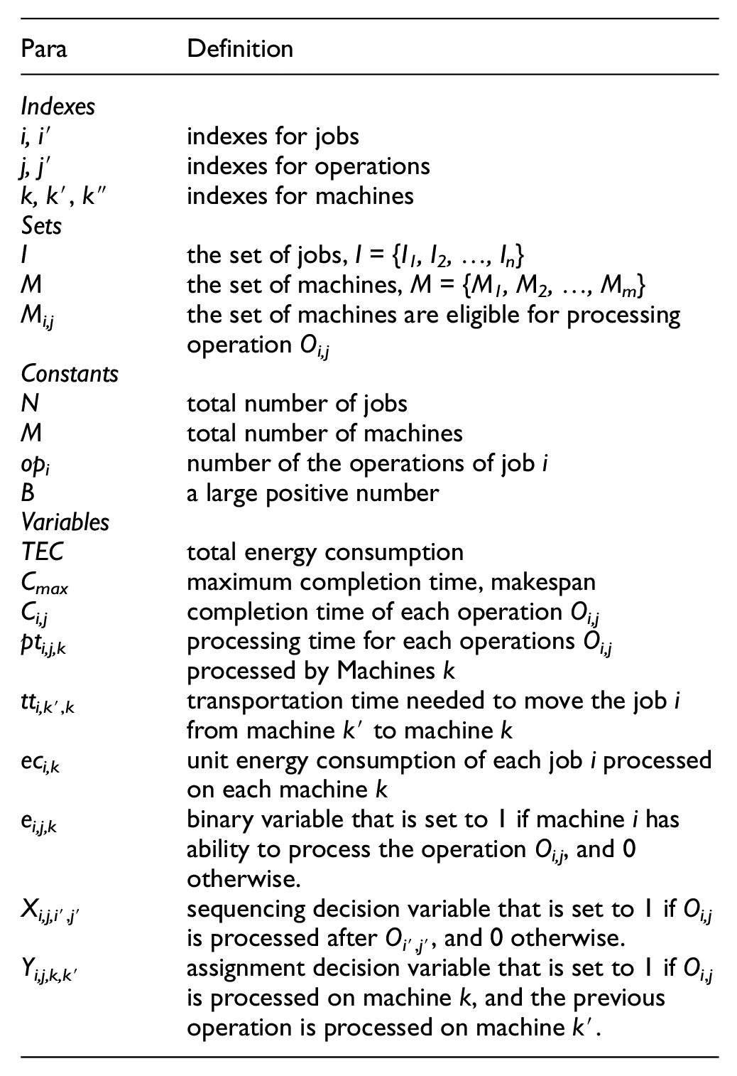
In this paper, we propose a mathematical model based on the FJSP with energy consumption and transportation time, which can be defined as follows. There is a set of jobs {I₁, I₂, …, I_n} to be executed on a set of machines {M₁, M₂, …, M_m} in which each job I_i consists of a sequence of op_i operations and each operation O_i,j is applied to on one of a subset of eligible machines M_i,j⊆M. In terms of transportation time, every operation O_i,j of each job I_i has its own transportation time tt_i,k′,k of transferring from machine k′ to another machine k. In addition, the energy consumption generated when jobs are processed on machines is taken into account. When jobs are being processed on machines, they produce disparate energy consumption ec_i,j per unit time. It worth noting that all the machines are assumed to be the same, and variables given in the mathematical model, that is, processing time of each operation, transportation time and unit energy consumption, are fixed and not affected by the state of machines. The parameters defined in this model are showed as follows.

$$\begin{array}{c}min\alpha ·C_{max}+(1-\alpha )·\mathrm{TEC}\\ \mathrm{TEC}=\sum _{i=1}^n\sum _{j=1}^{o{p}_i}\sum _{k=1}^m\sum _{k\prime =1}^m{Y}_{i,j,k,k\prime }\times p{t}_{i,j,k}\times e{c}_{i,k}\end{array}$$

(1)

$$\sum _{k=1}^m\sum _{k\prime =1}^m{Y}_{i,j,k,k\prime }=1\forall i,j>1$$

(2)

$$\sum _{k=1}^m{Y}_{i,1,k,0}=1\forall i$$

(3)

$$\sum _{k\prime =1}^m{Y}_{i,j,k,k\prime }\le e_{i,j,k}\forall i,j>1,k$$

(4)

$$Y_{i,1,k,0}\le e_{i,1,k}\forall i,j$$

(5)

$$Y_{i,j,k,k\prime }\le \sum _{k″=1}^m{Y}_{i,j-1,k\prime ,k″}\forall i,j>2,k,k\prime$$

(6)

$$Y_{i,2,k,k\prime }\le Y_{i,1,k\prime ,0}\forall i,k,k\prime$$

(7)

$$C_{i,j}\ge C_{i,j-1}+\sum _{k=1}^m\sum _{k\prime =1}^m{Y}_{i,j,k,k\prime }(p{t}_{i,j,k}+t{t}_{i,k\prime ,k})\forall i,j>1$$

(8)

$$C_{i,1}\ge \sum _{k=1}^m{Y}_{i,1,k,0}(p{t}_{i,1,k}+t{t}_{i,0,k})\forall i$$

(9)

$$\begin{array}{c}{C}_{i,j}\ge C_{i\prime ,j\prime }+p{t}_{i,j,k}-B(1-X_{i,j,i\prime ,j\prime })\hfill \\ -B(2-(\sum _{k\prime =1}^m{Y}_{i,j,k,k\prime })-(\sum _{k\prime =1}^m{Y}_{i\prime ,j\prime ,k,k\prime }))\hfill \\ \forall i\ne i\prime ;j>1,j\prime >1;k\hfill \end{array}$$

(10)

$$\begin{array}{c}{C}_{i,1}\ge C_{i\prime ,j\prime }+p{t}_{i,1,k}-B(1-X_{i,1,i\prime ,j\prime })\hfill \\ -B(2-Y_{i,1,k,0}-(\sum _{k\prime =1}^m{Y}_{i\prime ,j\prime ,k,k\prime }))\forall i\ne i\prime ;j\prime >1;k\hfill \end{array}$$

(11)

$$\begin{array}{c}{C}_{i,j}\ge C_{i\prime ,1}+p{t}_{i,j,k}-B(1-X_{i,j,k\prime ,1})\hfill \\ -B(2-(\sum _{k\prime =1}^m{Y}_{i,j,k,k\prime })-Y_{i\prime ,1,k,0})\forall i\ne i\prime ;j>1;k\hfill \end{array}$$

(12)

$$\begin{array}{c}{C}_{i,1}\ge C_{i\prime ,1}+p{t}_{i,1,k}-B(1-X_{i,1,i\prime ,1})\hfill \\ -B(2-Y_{i,1,k,0}-Y_{i\prime ,1,k,0})\forall i\ne i\prime ;k\hfill \end{array}$$

(13)

$$\begin{array}{c}{C}_{i\prime ,j\prime }\ge C_{i,j}+p{t}_{i\prime ,j\prime ,k}-B(X_{i,j,i\prime ,j\prime })\hfill \\ -B(2-(\sum _{k\prime =1}^m{Y}_{i,j,k,k\prime })-(\sum _{k\prime =1}^m{Y}_{i\prime ,j\prime ,k,k\prime }))\hfill \\ \forall i\ne i\prime ;j>1,j\prime >1;k\hfill \end{array}$$

(14)

$$\begin{array}{c}{C}_{i\prime ,j\prime }\ge C_{i,1}+p{t}_{i\prime ,j\prime ,k}-B(X_{i,1,i\prime ,j\prime })\hfill \\ -B(2-Y_{i,1,k,0}-(\sum _{k\prime =1}^m{Y}_{i\prime ,j\prime ,k,k\prime }))\forall i\ne i\prime ;j\prime >1;k\hfill \end{array}$$

(15)

$$\begin{array}{c}{C}_{i\prime ,1}\ge C_{i,j}+p{t}_{i\prime ,1,k}-B(X_{i,j,i\prime ,1})\hfill \\ -B(2-(\sum _{k\prime =1}^m{Y}_{i,j,k,k\prime })-Y_{i\prime ,1,k,0})\forall i\ne i\prime ;j>1;k\hfill \end{array}$$

(16)

$$\begin{array}{c}{C}_{i\prime ,1}\ge C_{i,1}+p{t}_{i\prime ,1,k}-B(X_{i,1,i\prime ,1})\hfill \\ -B(2-Y_{i,1,k,0}-Y_{i\prime ,1,k,0})\forall i\ne i\prime ;k\hfill \end{array}$$

(17)

$$C_{max}\ge C_{i,n_i}\forall i$$

(18)

$$C_{i,j}\ge 0\forall i,j$$

(19)

$$X_{i,j,i\prime ,j\prime },Y_{i,j,k,k\prime }\in \{0,1\}$$

(20)

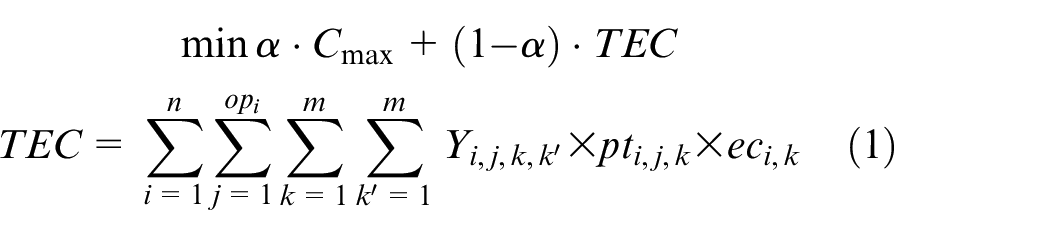
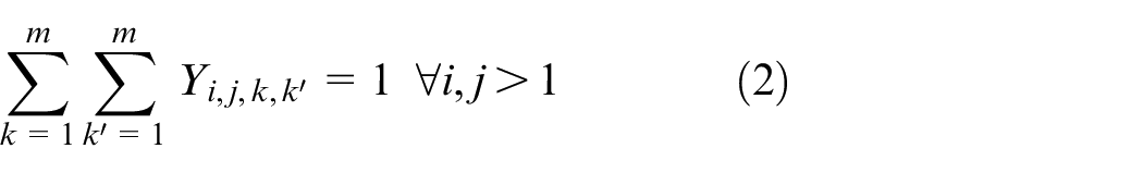
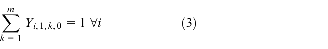
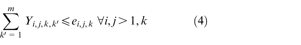
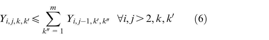
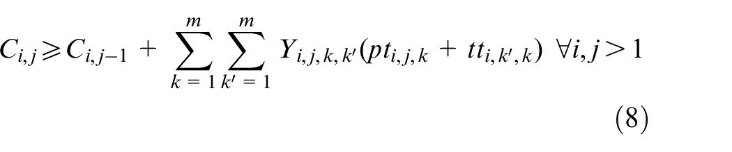
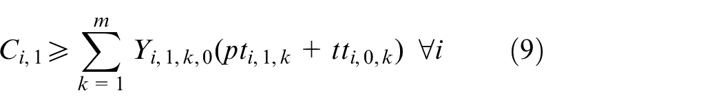
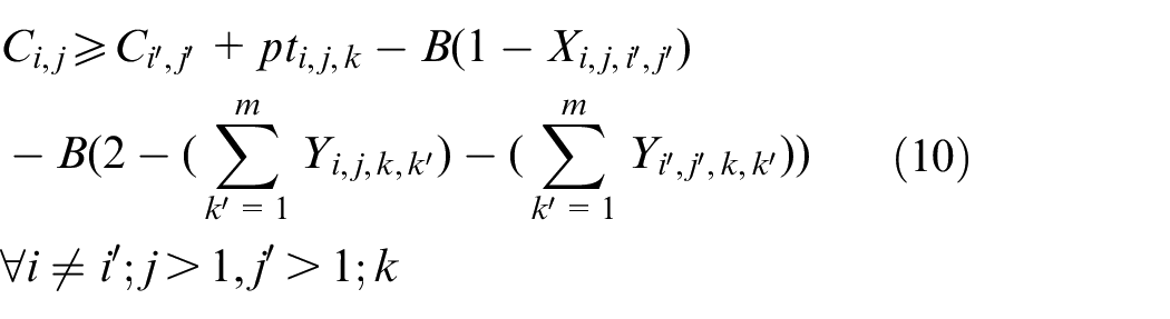
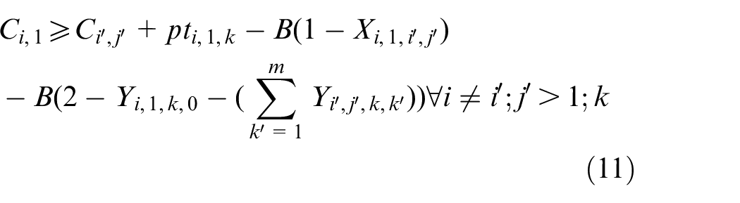
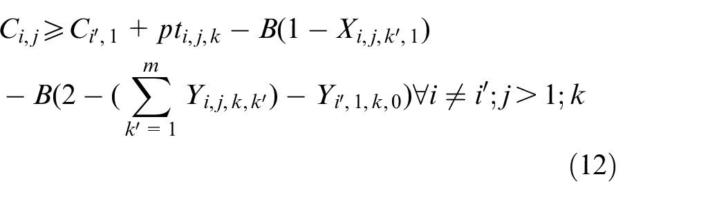
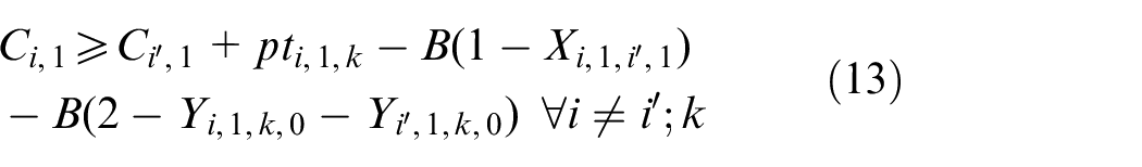
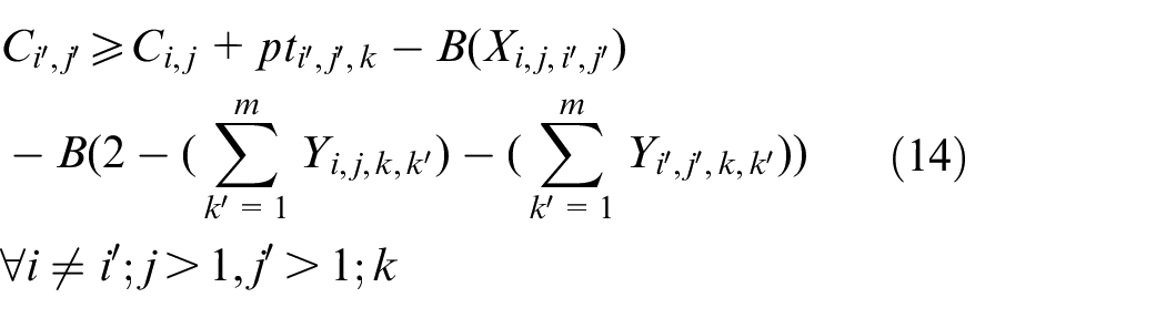
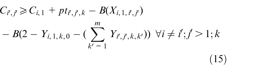
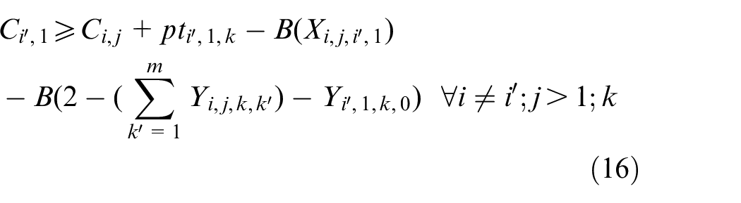
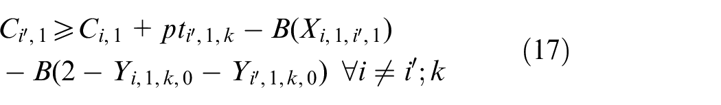
The objective aims to minimize the weighted value of makespan plus energy consumption. The constraint (1) is to calculate the total energy consumption of all operations when they are being processed on the machines. The constraints (2) and (3) ensure that each operation O_i,j is processed on only a specified machine. For any random operation selected from all of the operations, it is possible that not all of the machines have the ability to handle that operation, and there is a significant possibility that eligible machines comprise only a proper subset of all machines; hence, constraint (4) and (5) are included to make sure that each operation is to be allocated to a feasible machine. Constraints (6) and (7) limit the processing relation of the previous and next operations; if O_i,j is processed on the machine k, then O_i,j−1 must be processed on the machine k′. To calculate the completion time, we summarize the constraints (8) and (9) that each operation begins after the completion time and transportation time of the previous operation. Constraints (10)–(17) guarantee that every operation is to be processed on only one machine at a particular time. Constraint (18) ensures that the final result, the maximum completion time of the last operation, has been obtained. The range of values of three decision variables are defined by constraint (19) and constraint (20). The validity of this model has been verified by coding the problem formula in IBM ILOG CPLEX 12.7 and running various small instances, as discussed in section “Comparison with the exact solver CPLEX.”

Example of the FJSP-T model

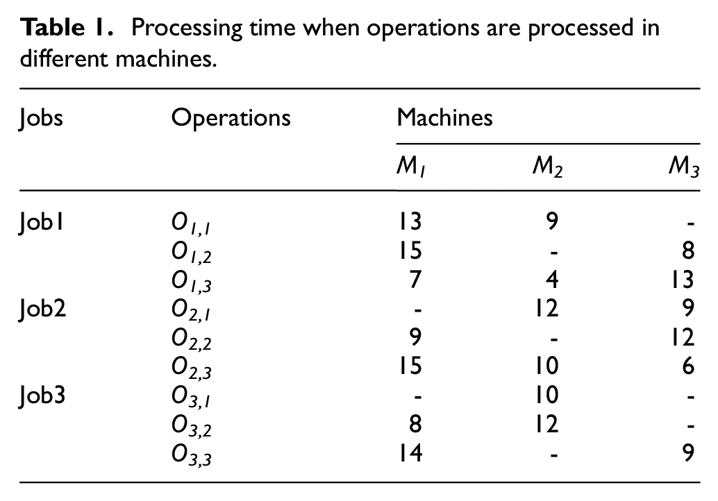
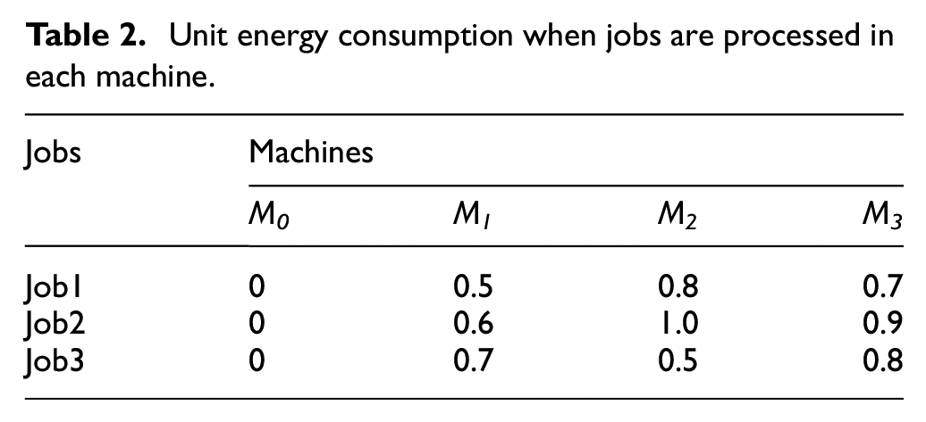
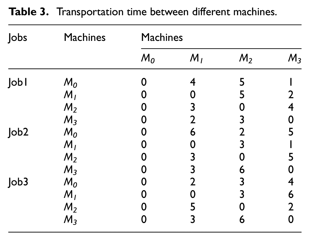
There gives a typical example to illustrate the FJSP with the constraint of transportation time, the processing time is shown in Table 1, in which the symbol “-” indicates that the machine does not have ability to process the job. The unit energy consumption generated by each job during the processing of each machine is listed in Table 2. Because the M₀ machine is a virtual machine that represents the assembly line, the energy consumption generated by M₀ is zero, as is the related transportation time. The transportation time required for each job to be moved from one machine to another is listed in Table 3, as shown in Figure 1, where O_1,1 is the first operation of the first job. Once the process starts, O_1,1 is first transferred to M₁ and then transferred to M₃ for further processing. Since O_2,1 has finished processing at this time, some idle time appears. Other operations follow the identical process. The result is an optimal solution in which once an operation is completed, the job begins to be transported immediately to another machine in prepare for further processing, as illustrated in Figure 1.

Para	Definition
Indexes
i, i′	indexes for jobs
j, j′	indexes for operations
k, k′, k″	indexes for machines
Sets
I	the set of jobs, I = {I1, I2, …, In}
M	the set of machines, M = {M1, M2, …, Mm}
Mi,j	the set of machines are eligible for processing operation Oi,j
Constants
N	total number of jobs
M	total number of machines
opi	number of the operations of job i
B	a large positive number
Variables
TEC	total energy consumption
Cmax	maximum completion time, makespan
Ci,j	completion time of each operation Oi,j
pti,j,k	processing time for each operations Oi,j processed by Machines k
tti,k ′,k	transportation time needed to move the job i from machine k′ to machine k
eci,k	unit energy consumption of each job i processed on each machine k
ei,j,k	binary variable that is set to 1 if machine i has ability to process the operation Oi,j, and 0 otherwise.
Xi,j,i ′,j′	sequencing decision variable that is set to 1 if Oi,j is processed after Oi′,j′, and 0 otherwise.
Yi,j,k,k ′	assignment decision variable that is set to 1 if Oi,j is processed on machine k, and the previous operation is processed on machine k′.

Table 1.

Processing time when operations are processed in different machines.

Jobs	Operations	Machines
		M1	M2	M3
Job1	O1,1	13	9	-
	O1,2	15	-	8
	O1,3	7	4	13
Job2	O2,1	-	12	9
	O2,2	9	-	12
	O2,3	15	10	6
Job3	O3,1	-	10	-
	O3,2	8	12	-
	O3,3	14	-	9

Table 2.

Unit energy consumption when jobs are processed in each machine.

Jobs	Machines
	M0	M1	M2	M3
Job1	0	0.5	0.8	0.7
Job2	0	0.6	1.0	0.9
Job3	0	0.7	0.5	0.8

Table 3.

Transportation time between different machines.

Jobs	Machines	Machines
		M0	M1	M2	M3
Job1	M0	0	4	5	1
	M1	0	0	5	2
	M2	0	3	0	4
	M3	0	2	3	0
Job2	M0	0	6	2	5
	M1	0	0	3	1
	M2	0	3	0	5
	M3	0	3	6	0
Job3	M0	0	2	3	4
	M1	0	0	3	6
	M2	0	5	0	2
	M3	0	3	6	0

Figure 1.

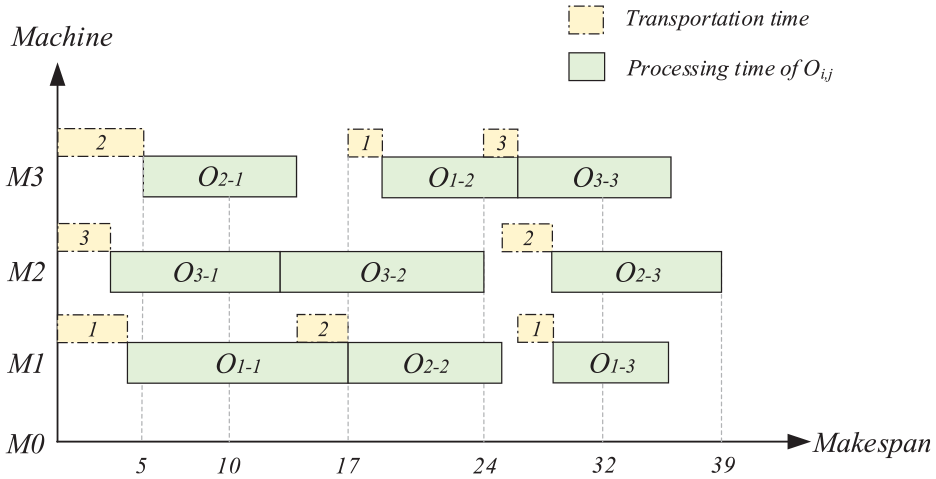
Gantt chart for the solution of the example.

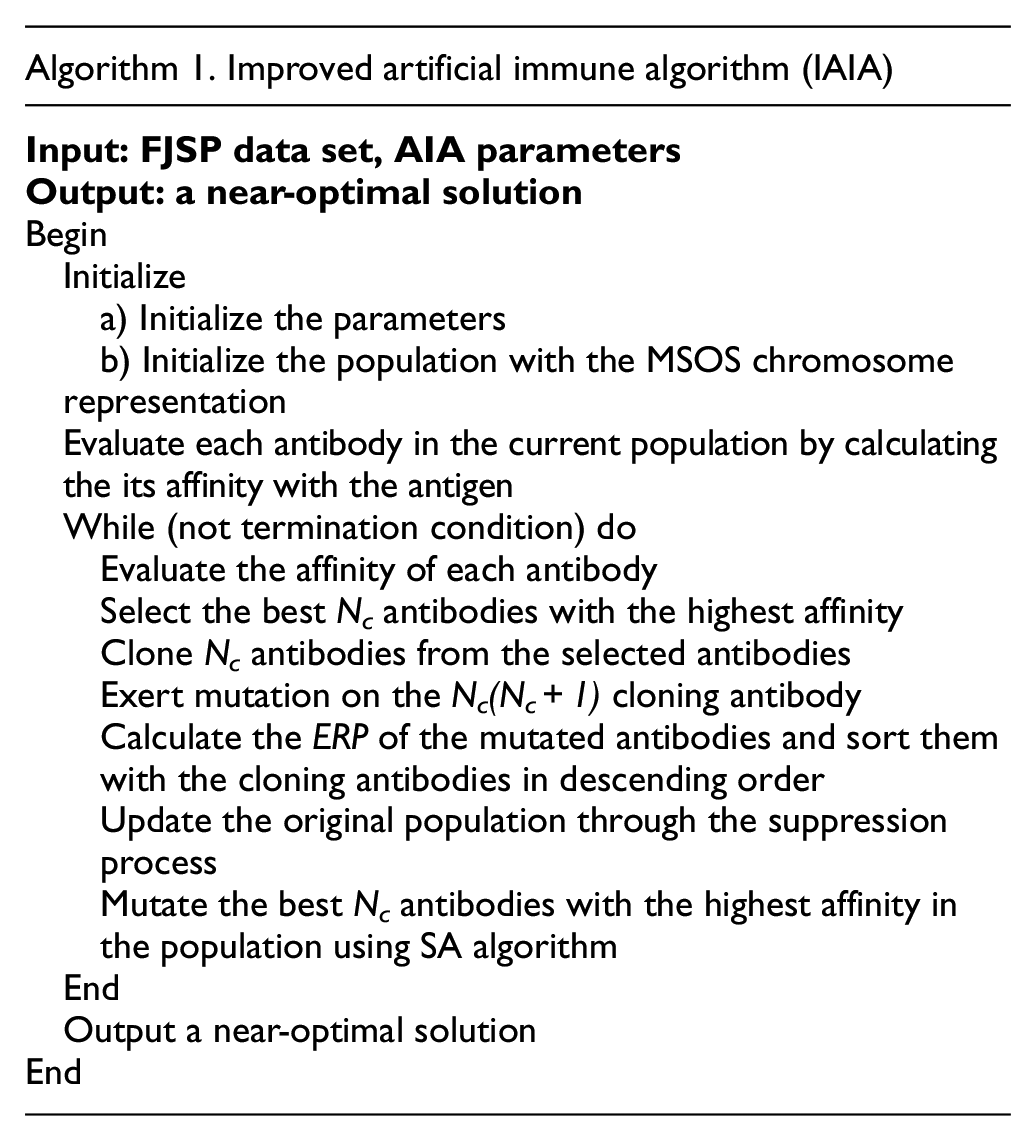
IAIA

The immune algorithm (IA) was first introduced by Burnt (1958). The AIA is a novel intelligent optimization algorithm, inspired by the human immune mechanism. The artificial immune system is an adaptive system modeled after the mechanism of human self-protection, including mechanisms as antigen recognition, clone selection, clone inhibition, and immune memory function. ²⁷ The resulting information processing mechanism based on the immune system is applied to the problem of scheduling.

In this study, the AIA, based on information entropy theory, is used to implement global search, taking the reciprocal of the makespan as the criterion of affinity evaluation. The similarity of the chromosomes is evaluated and the antibody concentration is determined on the basis. Then, the population is sorted according to two criteria, antigen affinity and antibody concentration, antibodies, with antibodies of quality then selected for further local search based on SA and an immune suppression operation.

Representation of antibodies and initialization of the population

In the population, a complete chromosome sequence is called an antibody (solution). An antibody is represented by a sequence of numbers which are composed of two parts, the machine-selection (MS) part and the operation-sequence (OS) part. As shown in Figure 2, in the MS part, the number of each gene represents the number of the corresponding processing machine. The first gene in the MS part is the first operation O_2,1 of the job I₂, and the number two on the gene position indicating that this operation is carried out by the second machine of a set of machines that are available for the O_2,1. There are two available machines that can implement the operation O_2,2 and the first machine is selected, resulting in the second gene position of the MS part to be one. Other numbers have the respective same meanings. In the OS part, each job I_i appears op_i times, where op_i indicates the number of operations of job I_i, and the order in which each job emerges determines the operation it is. The processing sequence illustrated in Figure 2 is O_3,1– O_1,1– O_2,1– O_3,2– O_2,2– O_2,3– O_1,2– O_1,3– O_3,3. The total length of the chromosome is $2\times \sum _{j=1}^{N}o{p}_j$ .

Figure 2.

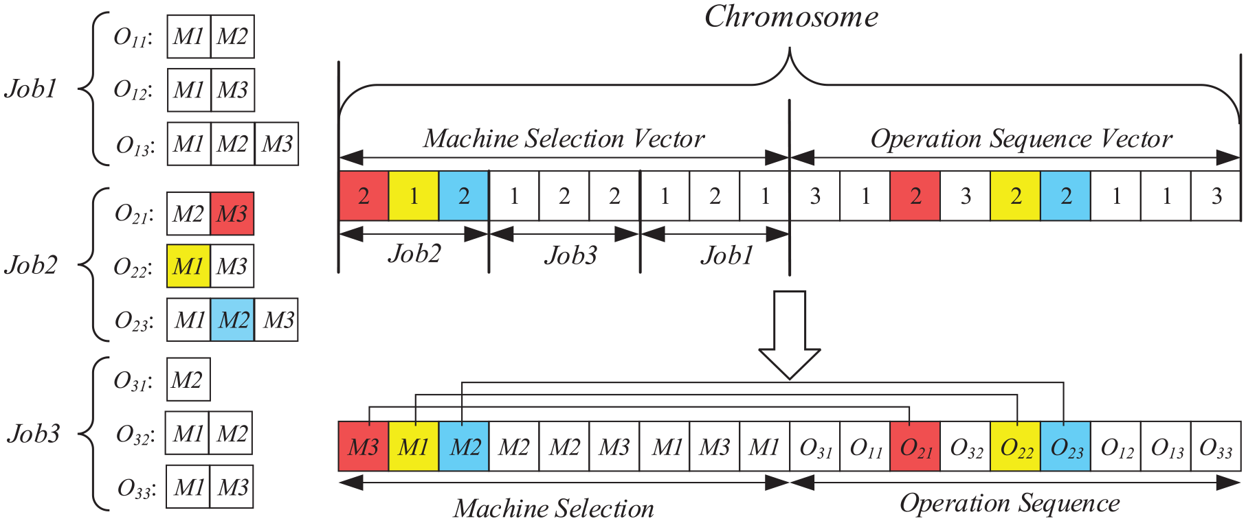
Representation of an antibody.

To maintain the diversity of the population and enable coding scheme to obtain the optimal solution quickly, global selection (GS), location selection (LS), and random selection (RS) are applied to the generated MS part. These three encoding schemes, all designed by Karimi et al., ¹⁶ require no repair mechanism thereby substantially reducing the time complexity. First, each job I_i is assigned a different integer in the interval [1,N] representing the priority of each job to be processed. Then, each operation is allocated to a feasible machine in turn. Meanwhile, the operation-selection part is initialized using RS. For the MS part, all of the jobs are assigned randomly, and each operation is arranged successively to a feasible machine respectively, with number k indicating that the kth available machine is assigned to corresponding operation. For the OS part, all of the operations are disorganized and inserted into the chromosome.

Affinity calculation

In this study, evaluation criteria of antibodies are determined by affinity between antibody and antigen (aff) and individual concentration (den). After evaluation, only antibodies with higher expected reproduction probability (ERP) will be subject to immune operation, where ERP is the probability that a selected antibody being selected. The formula for calculating the ERP is as follows:

$$\mathrm{ERP}=\beta \frac{\mathrm{af}{f}_p}{\sum \mathrm{af}{f}_p}+(1-\beta )\frac{\mathrm{de}{n}_p}{\sum \mathrm{de}{n}_p}$$

(21)

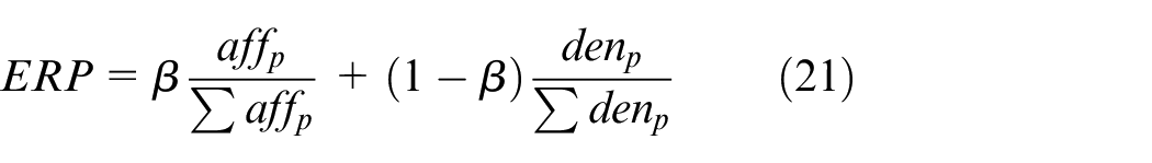
where aff_p is the affinity between antibody p and the antigen, den_p is the individual concentration of the antibody p, and the variable β is used to determine their respective weights. After normalization, antibodies with higher affinity and lower concentration can obtain better values of ERP.

Affinity of antigen

Each antibody has its own affinity for the antigen, which is related to the maximum completion time (C_max). To calculate the affinity between antibody and antigen, the following equation is used:

$$\mathrm{af}{f}_p=1/C_{max}(P)$$

(22)

This equation, makes it clear that the affinity of each antibody is determined by the makespan and that a greater affinity of the antibody corresponds to a lower makespan.

Antibody concentration

To decrease the number of the same antibodies and increase the diversity of the population, the proposed algorithm introduces affinity between antibody and other antibodies in the population. We calculate the particular affinity based on the immunity and entropy theory presented by Cui et al. ⁴¹ For each antibody, the number of antibodies that resemble another antibody divided by the total number of antibodies is the concentration of an antibody. More similar antibodies in the population, results in a higher concentration of an antibody and the more expected reproduction probability of an antibody, resulting in a degrading of the ERP. ⁴² The calculation of antibody concentration is detailed as follows:

• Step 1: Information entropy theory of antibodies

The evaluation of antibody concentration through information entropy is essentially to calculate the number of the same genes in the chromosome. The average entropy (H) is calculated using equation (23):

$$H_{a,b}(\eta )=\frac{1}{L}\sum _{k=1}^L{H}_{a,b,k}(\eta )$$

(23)

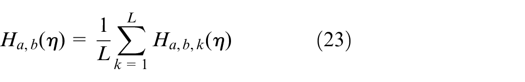
where η is the number of antibodies with its value being two in general, representing average information entropy of the two antibodies. Assuming that there are L genes in a chromosome, the information entropy of each gene is calculated using equation (24):

$$H_{a,b,k}(\eta )=\sum _{n=1}^S-p_{n,k}\ln (p_{n,k})$$

(24)

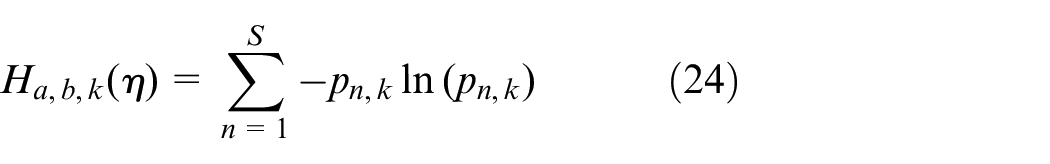
where p_n,k is the ratio that the nth number emerges at the kth locus, with p_n,k = (total number of occurrences of the nth number at the kth position among individuals)/η.

• Step 2: Similar extent of antibodies

The Similar extent of each antibody (Π_a,b) represents the similarity between individual a and b and it determined by the average information entropy between two antibodies. The similarity of an antibody is calculated as follows:

$$\underset{a,b}{\Pi }=\frac{1}{1+H_{a,b}(2)}$$

(25)

$$d_{a,b}=\{\begin{array}{cc}1\hfill & \underset{a,b}{\Pi }\ge \lambda \hfill \\ \multicolumn{1}{c}{0}& \mathrm{otherwise}\hfill \end{array}$$

(26)

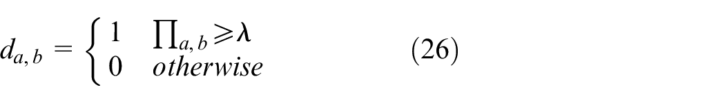
where H_a,b (2) is the common case in which η equals two, representing the average information entropy between individual a and individual b. To calculate the antibody similarity, an intermediate variable Π_a,b and a binary variable d_a,b are introduced. A greater H_a,b (2) value between two antibodies, corresponds to a smaller Π_a,b value between them. Π_a,b ranges from zero to one, and d_a,b is equals to one if the Π_a,b value exceeds the threshold λ; otherwise, it is zero.

• Step 3: Density of antibody.

The density of an antibody, denoted by den_p, is the rate of the number of antibodies that similar to antibody i in the population, which is defined as follows:

$$\mathrm{de}{n}_p=\frac{1}{N}\sum _{k=1}^N{d}_{p,k}$$

(27)

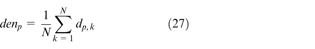
where d_p,k denotes the summary between the antibody p and the other antibodies, and N denotes the size of population.

Selecting and cloning

To search better antibodies, N_c antibodies with the highest affinity are selected in the initial population to undergo the clone operation. The clone number of each selected antibody can be defined as: N_c− k +1, in which k indicates that this antibody is the kth antibody with the highest affinity. Accordingly, N_c (N_c+1) clones are generated in preparation for next step.

Mutation

Mutation aims to search its neighboring solution by altering one or more genes on the chromosome. The chromosome is composed of MS part and OS part. Thus, we apply different mutation operators in each part of each clone antibodies.

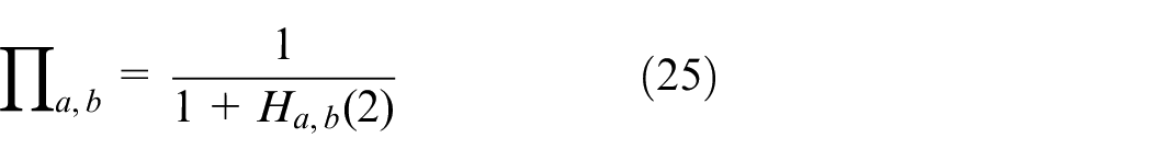
For the MS part, the random rule is used to change the sequence of the part. Two genes are randomly selected and replaced with other available machines. The new genes are also the serial numbers in the collection of available machines, rather than the number of the current machine. Considering the example in Figure 2, the MS mutation operator is shown in Figure 3(a), with the gene at the third position, as the third operation of J₂, is replaced by three in the collection of available machines that can process O_2,3.

Figure 3.

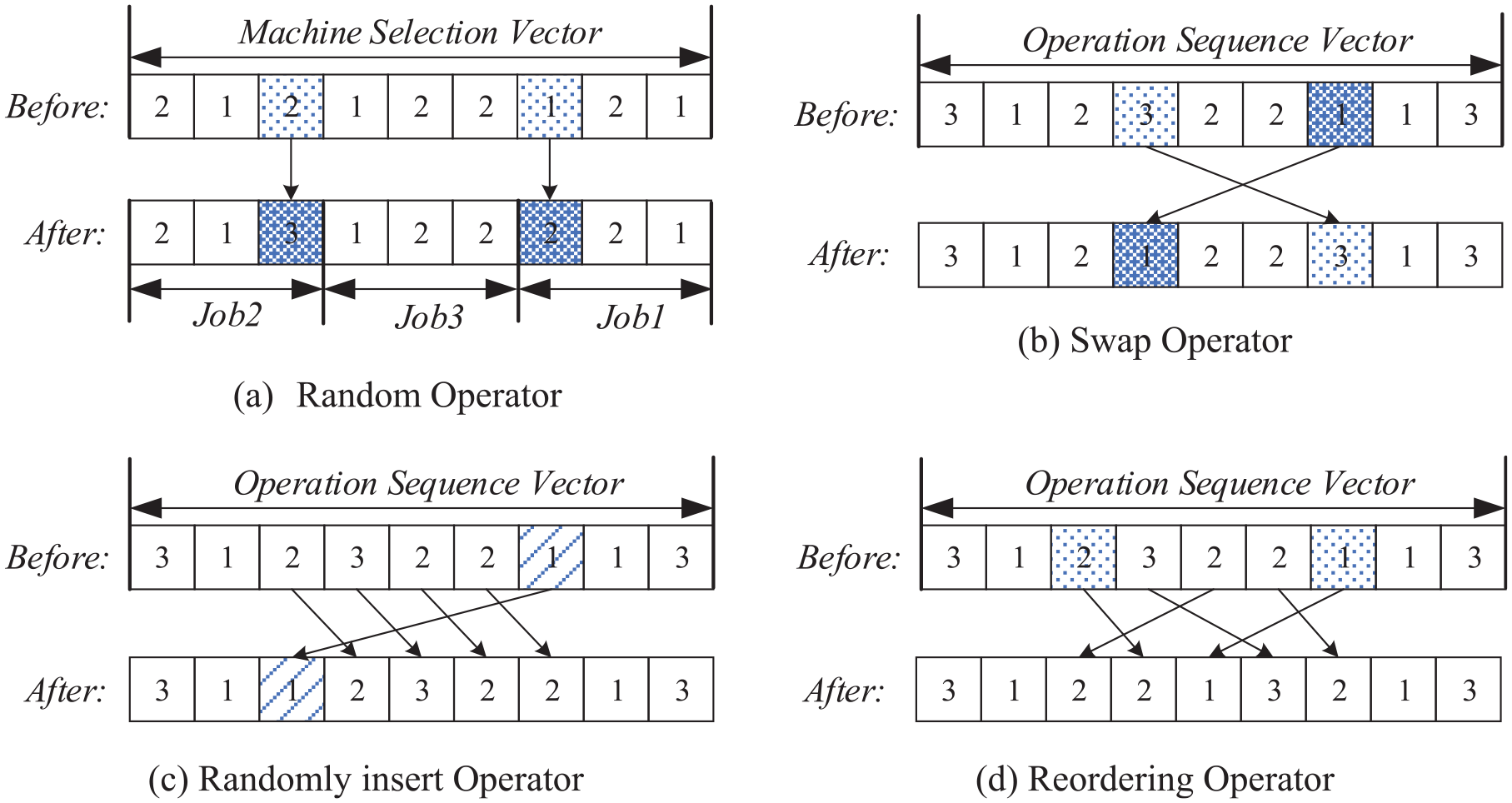
Illustration of the various mutation operators.

For another OS, three different canonical mutation operators are used to search other optimal solutions in the neighbor field.

• (1) Swap operator: To form a new neighborhood solution, two different gene positions are selected randomly in the current solution to be exchanged at the selection positions. ⁶

• (2) Randomly insert operator: A gene position is randomly selected and shifted it into a previous position. ⁴³

• (3) Reordering operator: We randomly select two different gene positions on the current chromosome and reorder the genes between the two selected positions.

To clarify the process, three OS mutation operators are shown in the Figure 3(b)−(d).

Update antibodies population

The clonal suppression operator selects the cloned and mutated antibodies, with lower-affinity antibodies are inhibited, leaving high affinity antibodies in a new antibody population. In this study, after the cloning and mutation processes, the selected high-quality antibodies are mixed with the cloned antibodies into a temporary antibody population. Then, the population is arranged in descending order according to the criterion of ERP, in which the N_c antibodies with the highest affinity is selected to replace the antibody with the lowest affinity in the initial population.

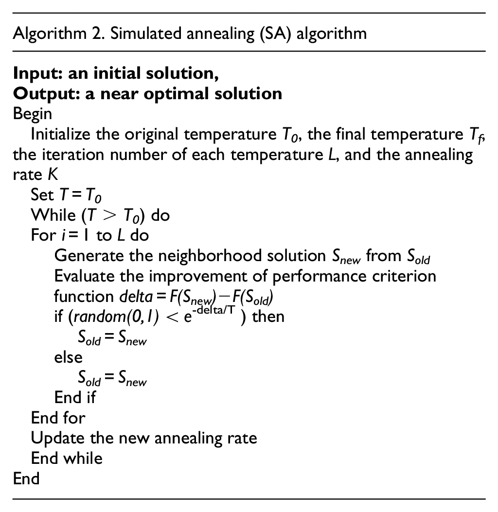
However, to avoid being trapped in local optimization, N_c antibodies with the highest affinity in the population are mutated through SA. The SA algorithm is an efficient heuristic algorithm. With its strong local search ability, it has been effectively applied to kinds of job shop scheduling problems combined with multiple optimization algorithms. In this study, on the basis of the original SA algorithm, a memory function is added to save the best solution obtained during search process and change the annealing rate. For each N_c antibody, a gene in the MS part is selected randomly selected and replaced with another available machine, and two genes randomly selected in the OS part are exchanged with each other. The mutated antibody replaces the previous one directly if the mutated antibody is better, and whether the best antibody needs to be updated is determined. Otherwise, the solution is accepted with a random probability, following the Metropolis criterion described in equation (28):

$$P=\{\begin{array}{cc}1,\hfill & F(S_{\mathrm{new}}<S_{\mathrm{old}})\hfill \\ \multicolumn{1}{c}{\exp (-\mathrm{delta}/T),}& F(S_{\mathrm{new}}>=S_{\mathrm{old}})\hfill \end{array}$$

(28)

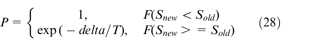
in which the probability of replacement is gradually reduced by temperature decline. When the system is at a higher temperature, the acceptance of the inferior solution is close to one, but the system no longer receives any inferior solutions when the temperature approaches T₀.

Compared to the traditional SA algorithm, in which the annealing rate is typically a fixed constant ranging from 0.75 to 0.95, therefore, the search of the algorithm at low temperatures is very slow and insufficient. Dai et al. ⁴⁴ improved the decline rate in accordance with the Hill function, after the completion of each isothermal search, the annealing using the following calculation criterion:

$$k_{\mathrm{new}}=k_{\mathrm{old}}\times \frac{T_0^n}{T_0^n+t^n}$$

(29)

$$T_t=T_{t-1}\times k_{\mathrm{new}}$$

(30)

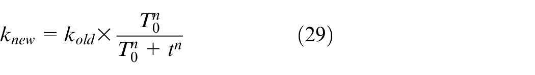
in which the t is the number of the annealing operation, and n represents is the Hill coefficient, whose value is typically greater than one. Consequently, the SA can be searched fully in the space of the solution to achieve the optimal effect.

Experiment analyses

In this chapter, the proposed IAIA is applied to solve the FJSP-T using C++. To testify the efficiency of the algorithm, the experimental tests are conducted on a PC with a 2.40-GHz Intel Core i7 CPU and 8 GB of RAM. Weight decomposition has been proved to be an effective way to optimize multi-objective problems. In this study, the proposed algorithm based on weight decomposition is used to optimize the FJSP-T model. In the part of proving the effectiveness of information entropy theory and SA algorithm, the coefficient of makespan α is set to 0.8, and the coefficient of total energy consumption is set to 0.2 because we prefer to take the completion time as the principal optimization objective. Then, in the section of multi-algorithm comparison, the performance of proposed algorithm is analyzed under three sets of weight coefficients, that is, 0.2, 0.5, and 0.8.

Instances

We randomly generated 30 instances based on the actual processing circumstances of a factory. The instances are divided into two parts, of which the first represents the job scale with values ranging from 10 to 100 and the number of jobs being n = {10,20, 30,50,100}, and the second represents the total number of machines, with the value m = {3,5,6,7,8,10}. In accordance with the characteristics of the FJSP, the number of operations contains a degree of randomness, with values randomly ranging from m/2 to m when the number of machines exceeds five. For example, the instance 10-5 involves 10 jobs processed on five machines, with the number of operations of jobs evenly valued within the interval [m/2, m]. In addition, the processing time of each operation is set to the interval [10,20], and the transportation time between two machines is set to [5,20], and the unit energy consumption when machines are processing is set to [0.5,1]. In actual production, for each operation, machines can be out of order or in preventive maintenance. Consequently, we randomly set up some machines with no processing capability with the value ranging from one to half number of the machines for each operation.

Parameter selection of the algorithm

Some key parameters in IAIA are evaluated because the final experimental effect will be affected by parameter selection, which involves some significant parameters. The selection of parameters determines the convergence speed and effect of the algorithm. Accordingly, four of the more critical parameters are selected to process the parameters adjustment experiment, with other parameters being selected from previous experience or other papers, as follows:

1. Population size Pop_size = 100

2. Ratio of initial assignment with GS: 60%

3. Ratio of initial assignment with LS: 30%

4. Ratio of initial assignment with RS: 10%

5. Original temperature T₀ = n × m

6. Final temperature T_f = 10

7. Iteration number of each temperature L = 100

8. Hill function t = 2

9. Selected probability of each operator P_m = 1/3

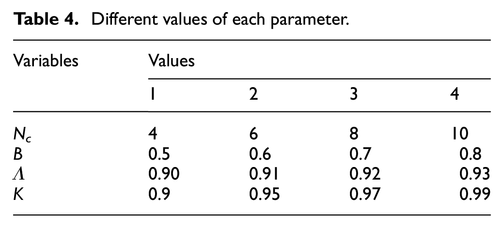
There are four significant parameters we considered in this study, that is, the number of selected antibodies with higher affinity (N_c), the weight of the objective (β), the concentration threshold (λ), and the annealing rate (K). The Taguchi method of Design of Experiment (DOE) was applied to verify the effect of these four parameters on the performance of the algorithm. For each parameter, we considered four levels, as shown in Table 4. A set of orthogonal arrays L₁₆ (4 ² ) was constructed to combine the parameters, and for each combination, which runs 30 times independently, the average value obtained is taken as the response value (RV). Table 5 shows all of the combinations of the four parameters and their corresponding RV values.

Table 4.

Different values of each parameter.

Variables	Values
	1	2	3	4
Nc	4	6	8	10
B	0.5	0.6	0.7	0.8
Λ	0.90	0.91	0.92	0.93
K	0.9	0.95	0.97	0.99

Table 5.

Combination situations of the algorithm parameters.

Number	Control factor level				RV
	Nc	β	Λ	K
1	1	1	1	1	1230.92
2	1	2	2	2	1232.77
3	1	3	3	3	1232.89
4	1	4	4	4	1235.67
5	2	1	2	3	1229.07
6	2	2	1	4	1227.66
7	2	3	4	1	1236.97
8	2	4	3	2	1228.71
9	3	1	3	4	1230.93
10	3	2	4	3	1247.56
11	3	3	1	2	1229.52
12	3	4	2	1	1233.04
13	4	1	4	2	1245.69
14	4	2	3	1	1237.24
15	4	3	2	4	1240.68
16	4	4	1	3	1232.59

Algorithm 1. Improved artificial immune algorithm (IAIA)
Input: FJSP data set, AIA parameters Output: a near-optimal solution
Begin
Initialize
a) Initialize the parameters
b) Initialize the population with the MSOS chromosome  representation
Evaluate each antibody in the current population by calculating  the its affinity with the antigen
While (not termination condition) do
Evaluate the affinity of each antibody
Select the best Nc antibodies with the highest affinity
Clone Nc antibodies from the selected antibodies
Exert mutation on the Nc(Nc+1) cloning antibody
Calculate the ERP of the mutated antibodies and sort them   with the cloning antibodies in descending order
Update the original population through the suppression   process
Mutate the best Nc antibodies with the highest affinity in   the population using SA algorithm
End
Output a near-optimal solution
End

Algorithm 2. Simulated annealing (SA) algorithm
Input: an initial solution,
Output: a near optimal solution
Begin
Initialize the original temperature T0, the final temperature Tf, the iteration number of each temperature L, and the annealing rate K
Set T = T0
While (T > T0) do
For i = 1 to L do
Generate the neighborhood solution Snew from Sold
Evaluate the improvement of performance criterion   function delta = F(Snew)−F(Sold)
if (random(0,1)<e-delta/T ) then
Sold = Snew
else
Sold = Snew
End if
End for
Update the new annealing rate
End while
End

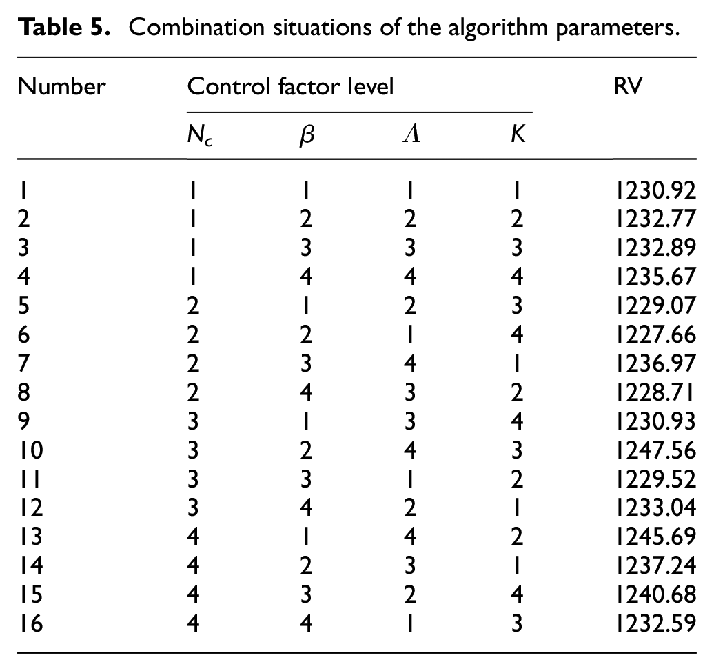
The instance 50-8 was used to evaluate each parameter of each combination. We show the factor level trend of each parameter in the Figure 4. According to this analysis, we can infer that N_c = 6, β = 0.8, λ = 0.90, K = 0.99 comprise the best set of parameters.

Figure 4.

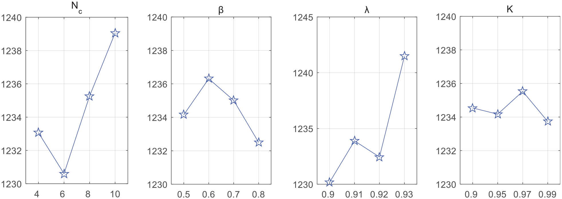
Factor level trend of parameters.

Comparison with the exact solver CPLEX

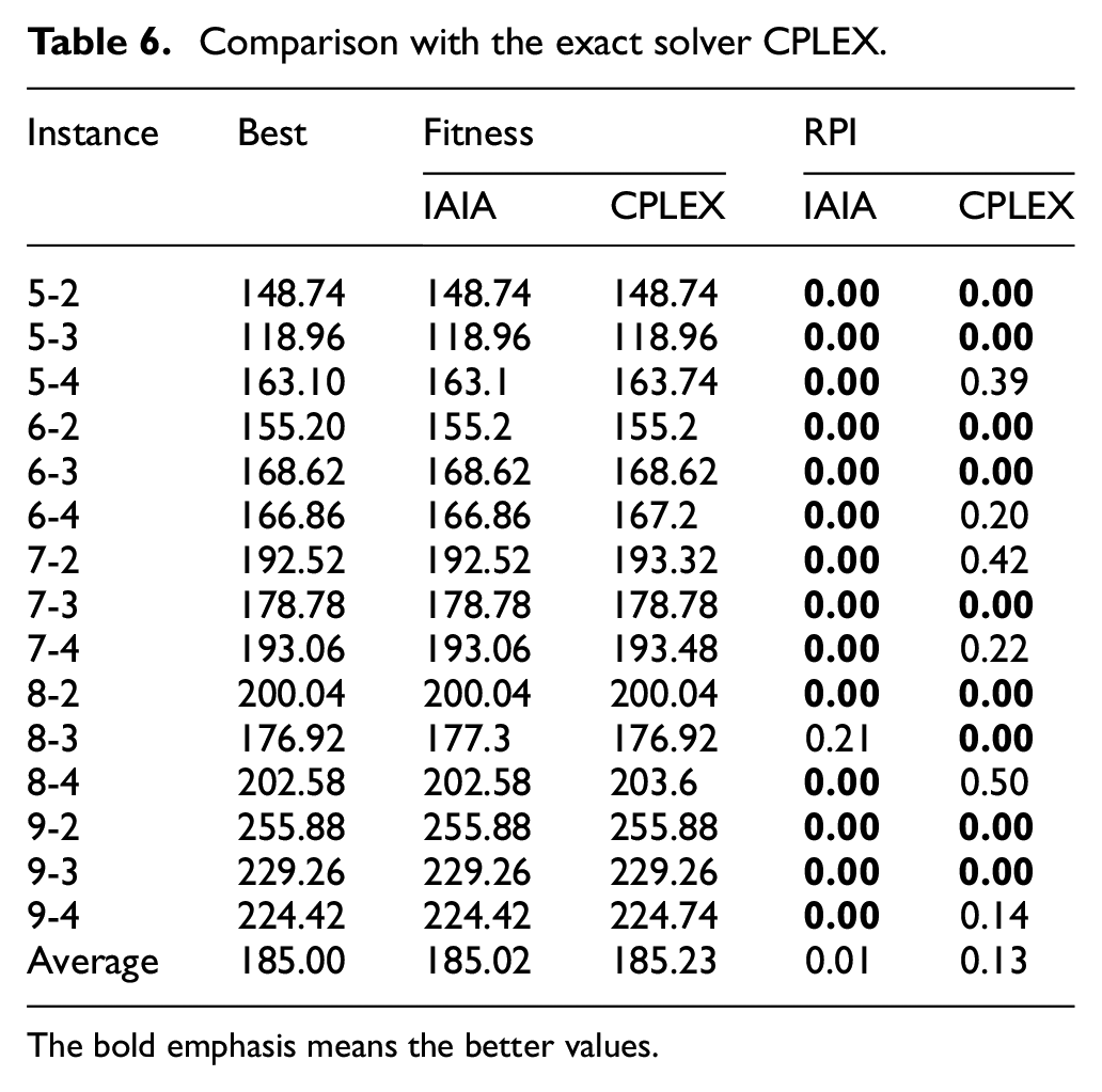
To certify the validity of the FJSP-T model, we coded the problem formula in IBM ILOG CPLEX 12.7 and ran various small-scale instances. Meanwhile, to verify the efficiency of the IAIA further, CPLEX was used as the benchmark for performing a comparison with the IAIA. Because CPLEX uses an exact algorithm based on branch and bound, calculating an accurate result requires substantial time. Consequently, the total computing time of CPLEX is limited to 1 h, and the number of threads is set to three. Each algorithm calculates the relative percentage increase (RPI) based on the best value, using the following equation:

$$\mathrm{RPI}=\frac{(f_{\mathrm{Current}}-f_{\mathrm{Best}})}{f_{\mathrm{Best}}}\times 100$$

(31)

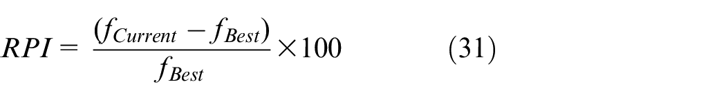
where f_Current is the fitness value of the current algorithm that we compared to, and f_Best is the best fitness value obtained from all of the given algorithms.

As shown in Table 6, the scale of each instance is listed in the first column, in which all the instances are generated randomly following the above generation rule. The best values selected from two algorithms are listed in the second column. The following two columns display the fitness values of two comparison algorithms, and the RPI values are displayed in the last two columns. In the illustrated 15 small instances, the proposed IAIA is able achieves better result as in most instances.

Table 6.

Comparison with the exact solver CPLEX.

Instance	Best	Fitness		RPI
		IAIA	CPLEX	IAIA	CPLEX
5-2	148.74	148.74	148.74	0.00	0.00
5-3	118.96	118.96	118.96	0.00	0.00
5-4	163.10	163.1	163.74	0.00	0.39
6-2	155.20	155.2	155.2	0.00	0.00
6-3	168.62	168.62	168.62	0.00	0.00
6-4	166.86	166.86	167.2	0.00	0.20
7-2	192.52	192.52	193.32	0.00	0.42
7-3	178.78	178.78	178.78	0.00	0.00
7-4	193.06	193.06	193.48	0.00	0.22
8-2	200.04	200.04	200.04	0.00	0.00
8-3	176.92	177.3	176.92	0.21	0.00
8-4	202.58	202.58	203.6	0.00	0.50
9-2	255.88	255.88	255.88	0.00	0.00
9-3	229.26	229.26	229.26	0.00	0.00
9-4	224.42	224.42	224.74	0.00	0.14
Average	185.00	185.02	185.23	0.01	0.13

The bold emphasis means the better values.

Efficiency of the local search

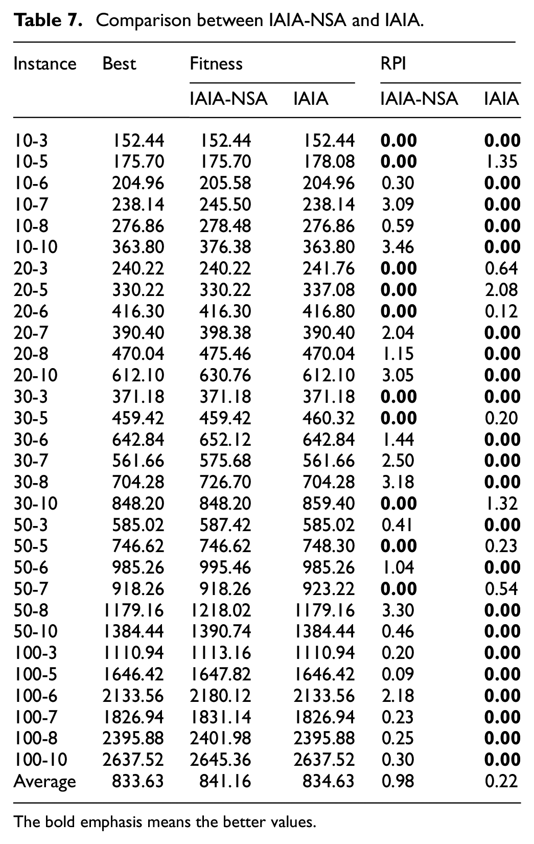
In this subsection, the SA algorithm is verified as to whether it can optimize the solution effectively. Then, the experiment is tested between the IAIA and the IAIA without the SA algorithm, denoted as IAIA-NSA.

As shown in Table 7, the scale of instances is listed in the first column, with the best value obtained from the comparison between two algorithms are displayed in second column. The average fitness value after 30 independent runs and the RPI value obtained from two algorithms are displayed in other columns. It can be observed that: (1) in the illustrated 30 instances, the IAIA obtained 22 optimal values and performed better than the IAIA-NSA, and (2) from the last row, the average RPI value obtained by IAIA is less than that of IAIA without the SA algorithm, which proves the efficiency of this improvement.

Table 7.

Comparison between IAIA-NSA and IAIA.

Instance	Best	Fitness		RPI
		IAIA-NSA	IAIA	IAIA-NSA	IAIA
10-3	152.44	152.44	152.44	0.00	0.00
10-5	175.70	175.70	178.08	0.00	1.35
10-6	204.96	205.58	204.96	0.30	0.00
10-7	238.14	245.50	238.14	3.09	0.00
10-8	276.86	278.48	276.86	0.59	0.00
10-10	363.80	376.38	363.80	3.46	0.00
20-3	240.22	240.22	241.76	0.00	0.64
20-5	330.22	330.22	337.08	0.00	2.08
20-6	416.30	416.30	416.80	0.00	0.12
20-7	390.40	398.38	390.40	2.04	0.00
20-8	470.04	475.46	470.04	1.15	0.00
20-10	612.10	630.76	612.10	3.05	0.00
30-3	371.18	371.18	371.18	0.00	0.00
30-5	459.42	459.42	460.32	0.00	0.20
30-6	642.84	652.12	642.84	1.44	0.00
30-7	561.66	575.68	561.66	2.50	0.00
30-8	704.28	726.70	704.28	3.18	0.00
30-10	848.20	848.20	859.40	0.00	1.32
50-3	585.02	587.42	585.02	0.41	0.00
50-5	746.62	746.62	748.30	0.00	0.23
50-6	985.26	995.46	985.26	1.04	0.00
50-7	918.26	918.26	923.22	0.00	0.54
50-8	1179.16	1218.02	1179.16	3.30	0.00
50-10	1384.44	1390.74	1384.44	0.46	0.00
100-3	1110.94	1113.16	1110.94	0.20	0.00
100-5	1646.42	1647.82	1646.42	0.09	0.00
100-6	2133.56	2180.12	2133.56	2.18	0.00
100-7	1826.94	1831.14	1826.94	0.23	0.00
100-8	2395.88	2401.98	2395.88	0.25	0.00
100-10	2637.52	2645.36	2637.52	0.30	0.00
Average	833.63	841.16	834.63	0.98	0.22

The bold emphasis means the better values.

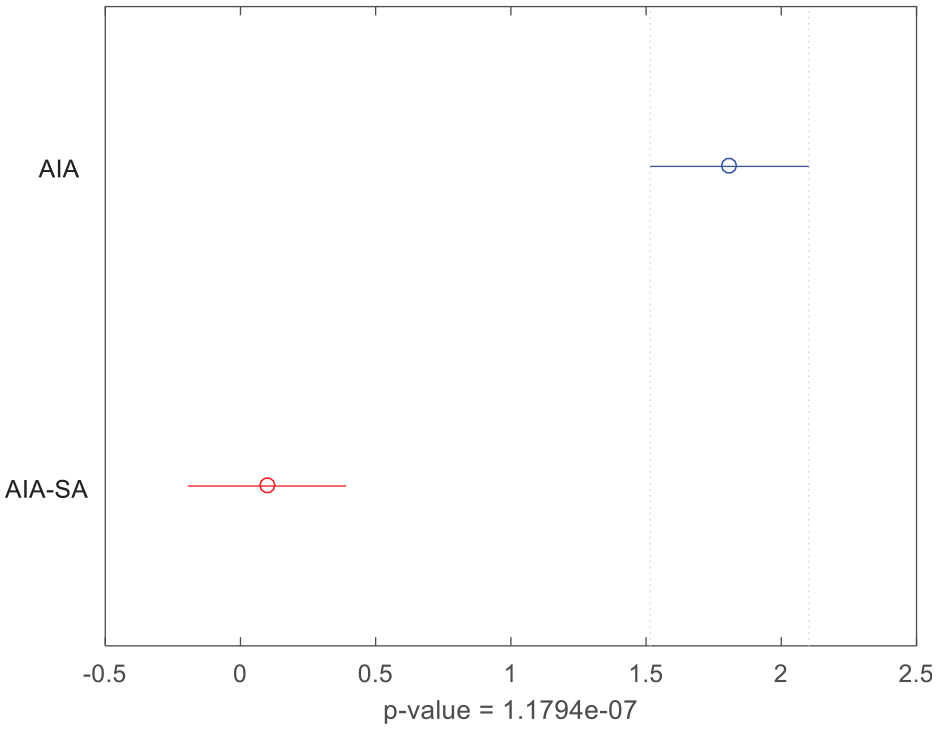
To testify the efficiency of the IAIA, a multifactor analysis of variance (ANOVA) is applied to describe the significant difference between two algorithms. The means and the 95% least-significant difference (LSD) interval are shown in Figure 5. The p-value, 1.1794e-07, is much less than 0.05, and that shows there are significant differences between two algorithms. Therefore, we can conclude that the proposed IAIA is significantly improved over the IAIA-NSA. The proposed algorithm has been greatly improved as a result of the utilization of the improved SA algorithm.

Figure 5.

Means and 95% LSD interval for IAIA-NSA and IAIA.

Efficiency of the information entropy strategy

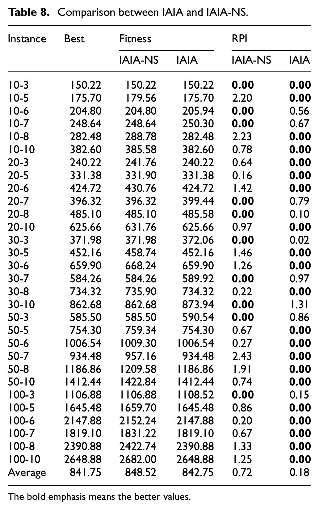
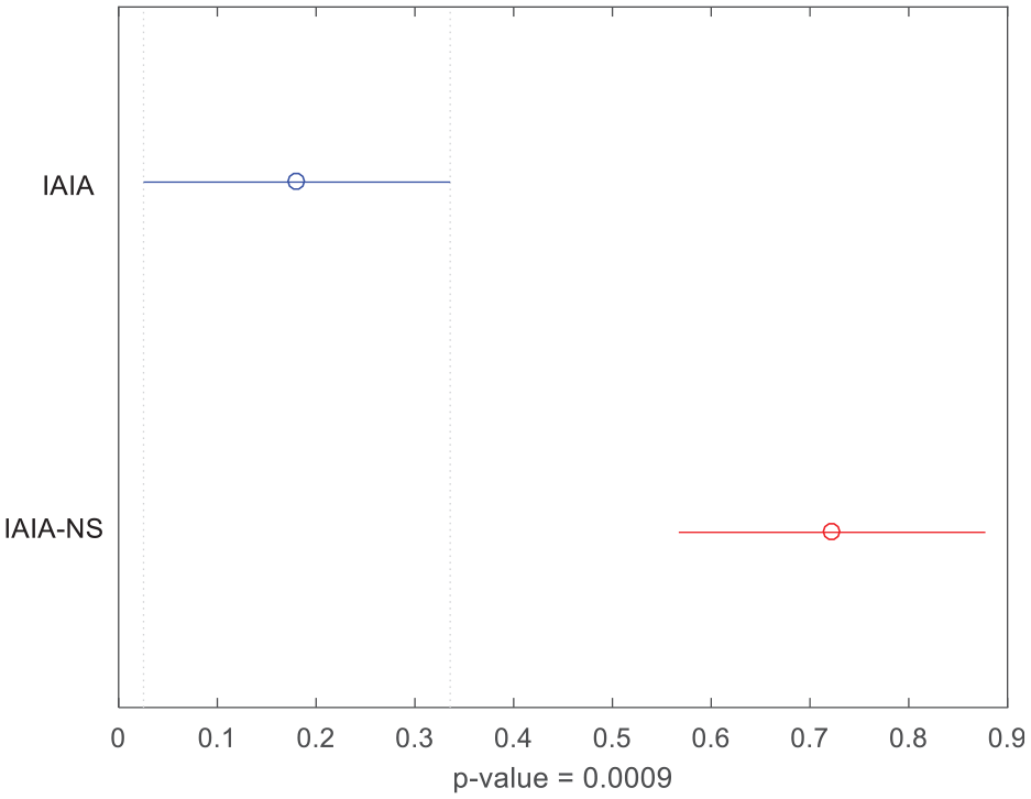
To testify the efficiency of the information entropy strategy, a method not using the information entropy strategy, which denoted as IAIA-NS, is described in this section. In this method, the antibody population of cloned antibodies and selected N_c antibodies is sorted according to affinity value between antibodies and antigens, rather than the ERP. Both the IAIA and IAIA-NS algorithms were implemented 30 times independently for 30 s each time. The minimum value obtained after 30 runs and the RPI values between the two algorithms are shown in the Table 8.

Table 8.

Comparison between IAIA and IAIA-NS.

Instance	Best	Fitness		RPI
		IAIA-NS	IAIA	IAIA-NS	IAIA
10-3	150.22	150.22	150.22	0.00	0.00
10-5	175.70	179.56	175.70	2.20	0.00
10-6	204.80	204.80	205.94	0.00	0.56
10-7	248.64	248.64	250.30	0.00	0.67
10-8	282.48	288.78	282.48	2.23	0.00
10-10	382.60	385.58	382.60	0.78	0.00
20-3	240.22	241.76	240.22	0.64	0.00
20-5	331.38	331.90	331.38	0.16	0.00
20-6	424.72	430.76	424.72	1.42	0.00
20-7	396.32	396.32	399.44	0.00	0.79
20-8	485.10	485.10	485.58	0.00	0.10
20-10	625.66	631.76	625.66	0.97	0.00
30-3	371.98	371.98	372.06	0.00	0.02
30-5	452.16	458.74	452.16	1.46	0.00
30-6	659.90	668.24	659.90	1.26	0.00
30-7	584.26	584.26	589.92	0.00	0.97
30-8	734.32	735.90	734.32	0.22	0.00
30-10	862.68	862.68	873.94	0.00	1.31
50-3	585.50	585.50	590.54	0.00	0.86
50-5	754.30	759.34	754.30	0.67	0.00
50-6	1006.54	1009.30	1006.54	0.27	0.00
50-7	934.48	957.16	934.48	2.43	0.00
50-8	1186.86	1209.58	1186.86	1.91	0.00
50-10	1412.44	1422.84	1412.44	0.74	0.00
100-3	1106.88	1106.88	1108.52	0.00	0.15
100-5	1645.48	1659.70	1645.48	0.86	0.00
100-6	2147.88	2152.24	2147.88	0.20	0.00
100-7	1819.10	1831.22	1819.10	0.67	0.00
100-8	2390.88	2422.74	2390.88	1.33	0.00
100-10	2648.88	2682.00	2648.88	1.25	0.00
Average	841.75	848.52	842.75	0.72	0.18

The bold emphasis means the better values.

The illustrated 30 instances shown in Table 8 shows that (1) the IAIA obtained 21 better solutions while IAIA-NS obtained only nine better solutions out of the 30 given instances; and (2) the average RPI value obtained by IAIA is less than that of IAIA without the strategy of information entropy, which proves the efficiency of the strategy.

Meanwhile, ANOVA was conducted with the confidence interval shown in Figure 6, with the obtained p-value is 0.0009, which is far less than 0.05. In conclusion, the application of the information entropy strategy performs better in solving this problem.

Figure 6.

Means and 95% LSD interval for IAIA-NSA and IAIA.

Comparison with other efficient algorithms

To verify the proposed algorithm has a great improvement, three other algorithms were selected to compare with the IAIA (1) the imperialist competitive algorithm, ¹⁶ (2) the enhanced GA, ¹⁹ and (3) the variable neighborhood search algorithm. ⁴⁵ The first and second comparison algorithms have been proved to have significant advantages in solving this problem, and the variable neighborhood search algorithm is also widely accepted because of its effective local search ability. Consequently, the advantages and competitive performance are better highlighted. Each algorithm runs 30 times independently and 30 s for each time, and the average value is used for comparison. In order to verify the performance of algorithms fairly, all the algorithms are implemented in accordance with the parameter, strategies and framework mentioned in the references, and the performance of each algorithm is compared under different weight coefficient. The experiment results are illustrated in the Tables 9 to 11, the average value for 30 runs for each instance of the four algorithms are displayed and the RPI values are obtained using the equation (31). As shown in Tables 9 to 11, we can observe that the proposed IAIA obtains the optimal values in most instances, obtaining RPI value equal to zero, with an absolutely advantage over the other algorithms. This shows the most effective performance in solving the FJSP-T model.

Table 9.

Comparison with other meta-heuristic algorithms under α = 0.8.

Instance	Best	Fitness				RPI
		ICA+LS	EGA	VNS	IAIA	ICA+LS	EGA	VNS	IAIA
10-3	151.13	151.13	153.15	151.83	152.55	0.00	1.32	0.46	0.93
10-5	179.17	181.25	186.63	179.17	179.49	1.15	4.00	0.00	0.18
10-6	206.78	211.05	217.87	210.59	206.78	2.02	5.09	1.81	0.00
10-7	246.90	252.72	261.99	259.95	246.90	2.30	5.76	5.02	0.00
10-8	278.73	288.52	299.39	296.18	278.73	3.40	6.90	5.89	0.00
10-10	360.05	381.69	401.46	400.36	360.05	5.67	10.32	10.07	0.00
20-3	241.80	241.81	244.54	241.80	242.55	0.00	1.12	0.00	0.31
20-5	333.71	342.68	356.46	343.97	333.71	2.62	6.38	2.98	0.00
20-6	411.49	434.67	450.51	441.36	411.49	5.33	8.66	6.77	0.00
20-7	384.35	409.66	427.92	421.30	384.35	6.18	10.18	8.77	0.00
20-8	448.63	490.67	511.13	503.14	448.63	8.57	12.23	10.84	0.00
20-10	582.99	640.55	667.03	655.78	582.99	8.99	12.60	11.10	0.00
30-3	371.54	374.48	376.21	371.54	373.60	0.78	1.24	0.00	0.55
30-5	457.51	469.58	486.12	464.35	457.51	2.57	5.89	1.47	0.00
30-6	640.00	677.05	702.44	678.60	640.00	5.47	8.89	5.69	0.00
30-7	550.59	585.43	610.72	597.99	550.59	5.95	9.84	7.93	0.00
30-8	677.83	739.58	771.37	752.18	677.83	8.35	12.13	9.89	0.00
30-10	810.50	882.49	905.97	886.57	810.50	8.16	10.54	8.58	0.00
50-3	582.53	601.05	598.56	582.53	586.15	3.08	2.68	0.00	0.62
50-5	747.41	763.98	783.79	757.58	747.41	2.17	4.64	1.34	0.00
50-6	979.18	1014.15	1039.07	1009.34	979.18	3.45	5.76	2.99	0.00
50-7	914.09	957.76	978.49	955.53	914.09	4.56	6.58	4.34	0.00
50-8	1164.66	1211.70	1241.20	1204.16	1164.66	3.88	6.17	3.28	0.00
50-10	1371.29	1424.66	1455.96	1410.93	1371.29	3.75	5.82	2.81	0.00
100-3	1098.01	1127.33	1135.77	1098.01	1110.22	2.60	3.32	0.00	1.10
100-5	1647.20	1663.82	1681.23	1647.20	1654.89	1.00	2.02	0.00	0.46
100-6	2137.72	2180.51	2204.13	2139.63	2137.72	1.96	3.01	0.09	0.00
100-7	1816.18	1845.26	1870.51	1826.68	1816.18	1.58	2.90	0.57	0.00
100-8	2379.81	2426.75	2465.67	2379.81	2383.35	1.93	3.48	0.00	0.15
100-10	2640.70	2688.32	2733.59	2640.70	2641.24	1.77	3.40	0.00	0.02
Average	827.08	855.34	873.96	850.29	828.15	3.64	6.10	3.76	0.14

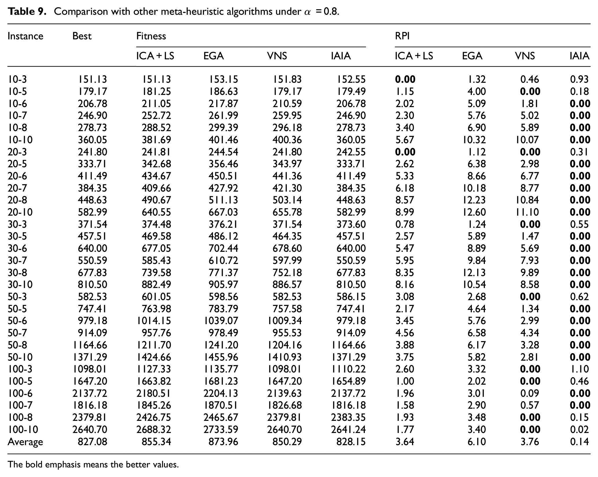
The bold emphasis means the better values.

Table 10.

Comparison with other meta-heuristic algorithms under α = 0.2.

Instance	Best	Fitness				RPI
		ICA+LS	EGA	VNS	IAIA	ICA+LS	EGA	VNS	IAIA
10-3	210.04	210.05	210.17	210.04	210.07	0.01	0.06	0.00	0.02
10-5	297.47	297.57	299.61	297.47	298.11	0.03	0.72	0.00	0.21
10-6	377.26	377.52	380.81	377.26	377.76	0.07	0.93	0.00	0.13
10-7	438.35	438.35	444.71	439.13	438.68	0.00	1.43	0.18	0.08
10-8	495.66	497.76	510.59	500.34	495.66	0.42	2.92	0.93	0.00
10-10	640.62	649.20	679.10	651.46	640.62	1.32	5.67	1.66	0.00
20-3	347.44	347.45	347.88	347.44	347.59	0.00	0.13	0.00	0.04
20-5	597.34	597.57	602.82	597.66	597.34	0.04	0.91	0.05	0.00
20-6	757.91	764.66	779.27	763.90	757.91	0.88	2.74	0.78	0.00
20-7	771.26	779.73	804.31	780.58	771.26	1.09	4.11	1.19	0.00
20-8	893.26	923.88	958.32	914.87	893.26	3.31	6.79	2.36	0.00
20-10	1163.51	1242.45	1292.42	1230.76	1163.51	6.35	9.97	5.46	0.00
30-3	575.20	575.20	575.42	575.20	575.20	0.00	0.04	0.00	0.00
30-5	843.15	846.51	855.45	843.98	843.15	0.40	1.44	0.10	0.00
30-6	1220.02	1246.10	1270.45	1233.33	1220.02	2.09	3.97	1.08	0.00
30-7	1059.06	1099.16	1137.65	1087.44	1059.06	3.65	6.91	2.61	0.00
30-8	1360.03	1448.41	1499.31	1413.17	1360.03	6.10	9.29	3.76	0.00
30-10	1642.19	1848.68	1900.91	1770.78	1642.19	11.17	13.61	7.26	0.00
50-3	882.87	883.73	884.68	882.87	882.96	0.10	0.21	0.00	0.01
50-5	1406.62	1431.41	1448.69	1413.01	1406.62	1.73	2.90	0.45	0.00
50-6	1822.82	1936.84	1963.43	1867.60	1822.82	5.89	7.16	2.40	0.00
50-7	1773.98	1938.17	1966.61	1840.64	1773.98	8.47	9.80	3.62	0.00
50-8	2306.79	2574.35	2615.38	2455.89	2306.79	10.39	11.80	6.07	0.00
50-10	2791.71	3168.18	3200.48	3036.74	2791.71	11.88	12.77	8.07	0.00
100-3	1657.71	1669.55	1668.83	1657.71	1658.41	0.71	0.67	0.00	0.04
100-5	2960.36	3186.95	3196.45	3025.99	2960.36	7.11	7.39	2.17	0.00
100-6	3988.18	4502.78	4487.97	4212.32	3988.18	11.43	11.14	5.32	0.00
100-7	3547.00	3981.59	4008.35	3796.74	3547.00	10.91	11.51	6.58	0.00
100-8	4916.04	5429.57	5452.52	5238.69	4916.04	9.46	9.84	6.16	0.00
100-10	5870.39	6377.07	6394.48	6228.60	5870.39	7.95	8.20	5.75	0.00
Average	1725.31	1859.60	1878.44	1803.88	1725.39	4.22	5.59	2.57	0.02

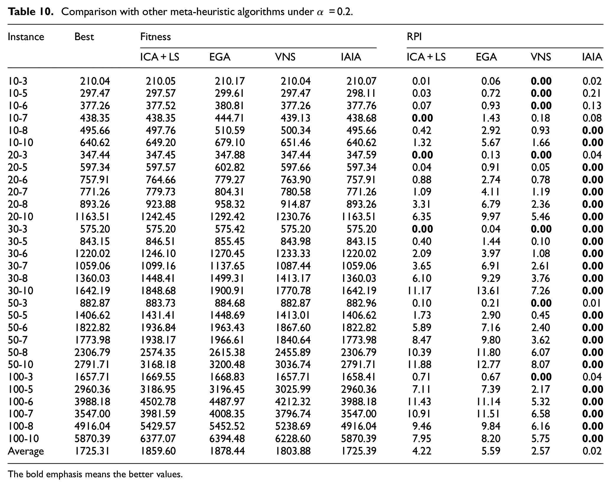
The bold emphasis means the better values.

Table 11.

Comparison with other meta-heuristic algorithms under α = 0.5.

Instance	Best	Fitness				RPI
		ICA+LS	EGA	VNS	IAIA	ICA+LS	EGA	VNS	IAIA
10-3	182.99	182.99	183.38	183.00	183.41	0.00	0.21	0.01	0.23
10-5	242.38	243.40	249.01	242.38	244.38	0.42	2.66	0.00	0.82
10-6	296.43	298.66	305.87	296.43	296.49	0.75	3.09	0.00	0.02
10-7	345.91	350.27	364.21	351.29	345.91	1.24	5.03	1.53	0.00
10-8	392.99	397.28	416.04	404.06	392.99	1.08	5.54	2.74	0.00
10-10	508.20	524.21	559.02	541.39	508.20	3.05	9.09	6.13	0.00
20-3	296.26	296.26	297.26	296.29	296.71	0.00	0.34	0.01	0.15
20-5	467.64	476.26	486.90	471.23	467.64	1.81	3.96	0.76	0.00
20-6	590.46	610.20	634.82	615.98	590.46	3.24	6.99	4.14	0.00
20-7	580.70	602.66	633.07	616.61	580.70	3.64	8.27	5.82	0.00
20-8	676.94	725.49	763.33	732.36	676.94	6.69	11.32	7.57	0.00
20-10	872.25	967.67	1011.55	986.43	872.25	9.86	13.77	11.57	0.00
30-3	473.49	475.11	476.79	473.49	475.12	0.34	0.69	0.00	0.34
30-5	647.62	663.40	680.15	656.20	647.62	2.38	4.78	1.31	0.00
30-6	926.32	974.11	1012.33	973.55	926.32	4.91	8.50	4.85	0.00
30-7	805.00	864.09	903.69	867.12	805.00	6.84	10.92	7.16	0.00
30-8	1019.08	1122.54	1174.56	1123.51	1019.08	9.22	13.24	9.29	0.00
30-10	1212.46	1393.90	1443.16	1402.20	1212.46	13.02	15.99	13.53	0.00
50-3	737.42	746.44	747.39	737.42	737.57	1.21	1.33	0.00	0.02
50-5	1076.32	1113.18	1137.75	1097.07	1076.32	3.31	5.40	1.89	0.00
50-6	1382.47	1509.56	1541.53	1477.59	1382.47	8.42	10.32	6.44	0.00
50-7	1334.23	1483.64	1521.70	1457.69	1334.23	10.07	12.32	8.47	0.00
50-8	1726.51	1928.91	1968.78	1910.14	1726.51	10.49	12.31	9.61	0.00
50-10	2071.06	2328.77	2368.72	2306.78	2071.06	11.07	12.57	10.22	0.00
100-3	1382.03	1415.09	1412.37	1382.03	1384.33	2.34	2.15	0.00	0.17
100-5	2299.06	2461.99	2487.24	2395.19	2299.06	6.62	7.57	4.01	0.00
100-6	3064.86	3374.44	3405.92	3302.44	3064.86	9.17	10.01	7.19	0.00
100-7	2689.59	2950.13	2971.90	2901.17	2689.59	8.83	9.50	7.29	0.00
100-8	3664.66	3960.40	3995.94	3905.27	3664.66	7.47	8.29	6.16	0.00
100-10	4276.66	4560.34	4588.66	4509.30	4276.66	6.22	6.80	5.16	0.00
Average	1307.05	1405.22	1430.05	1391.13	1307.28	5.16	7.41	4.77	0.06

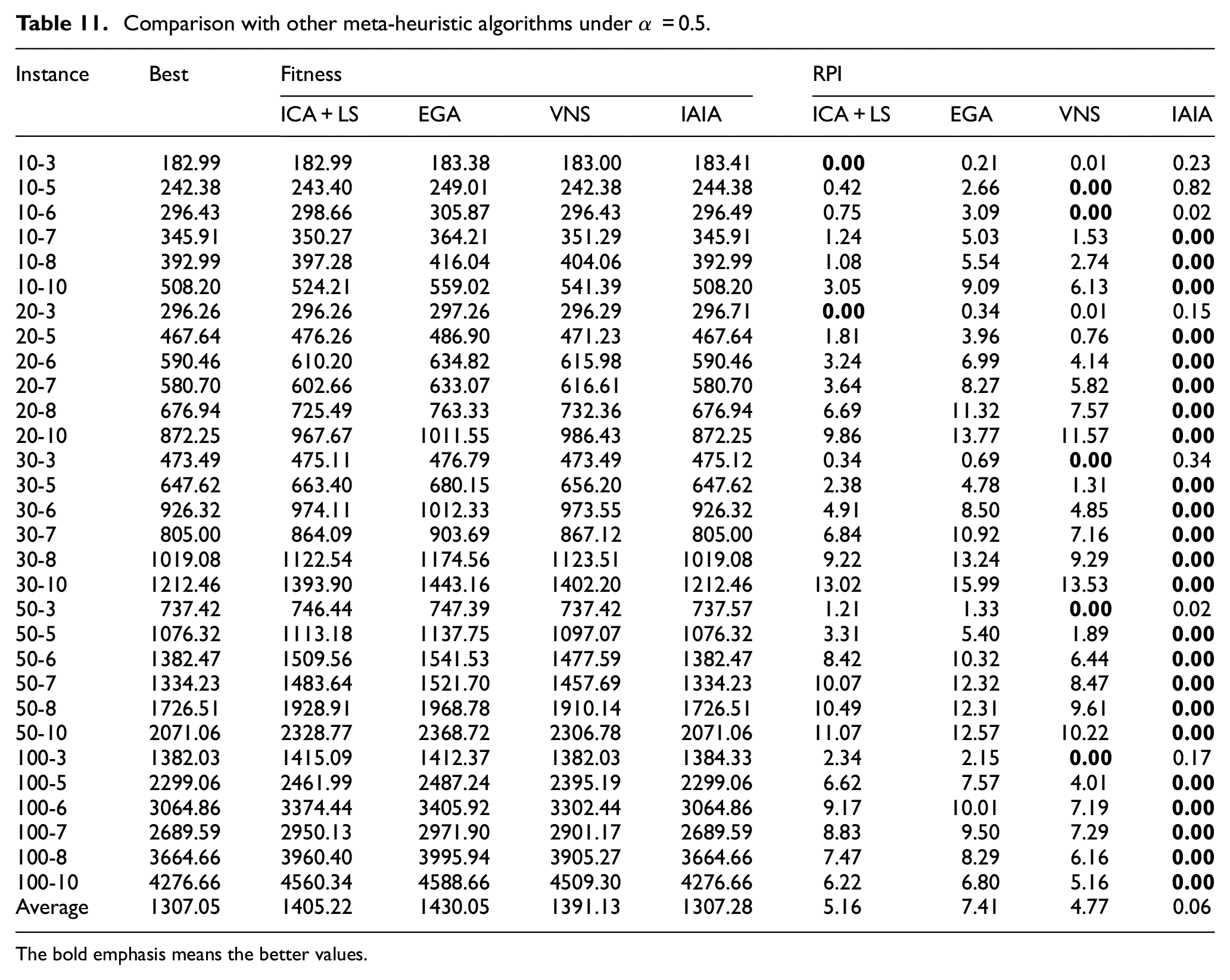
The bold emphasis means the better values.

In order to visualize the results of the comparison, ANOVA is applied to evaluate the performance of each algorithm. As shown in Figure 7(a)−(c), which represents different ANOVA diagram under three sets of weight coefficients, that is, 0.8, 0.2, and 0.5, and the p-value under three different sets of weight coefficients are all far less than 0.05, showing that the four compared algorithms have significant differences. Eight instances are selected randomly, and their corresponding convergence curves are showed in the Figure 8(a)−(h). In the illustrated convergence curves, the initial solution of IAIA is superior to the other three algorithms through the application of three initialization strategies. Meanwhile, the IAIA shows effective global search and local search abilities. Figure 9 illustrates a Gantt chart of an optimal solution of the instance 20-8, and this solution optimized by IAIA is feasible and efficient.

Figure 7.

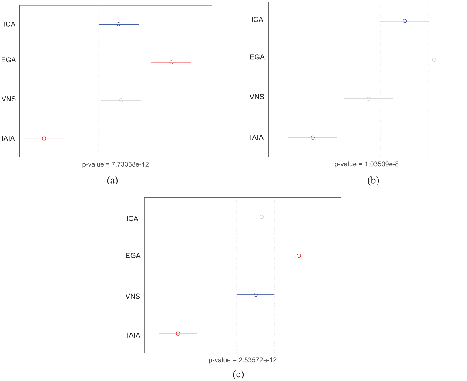
Means and 95% LSD interval for the compared algorithms under different coefficients.

Figure 8.

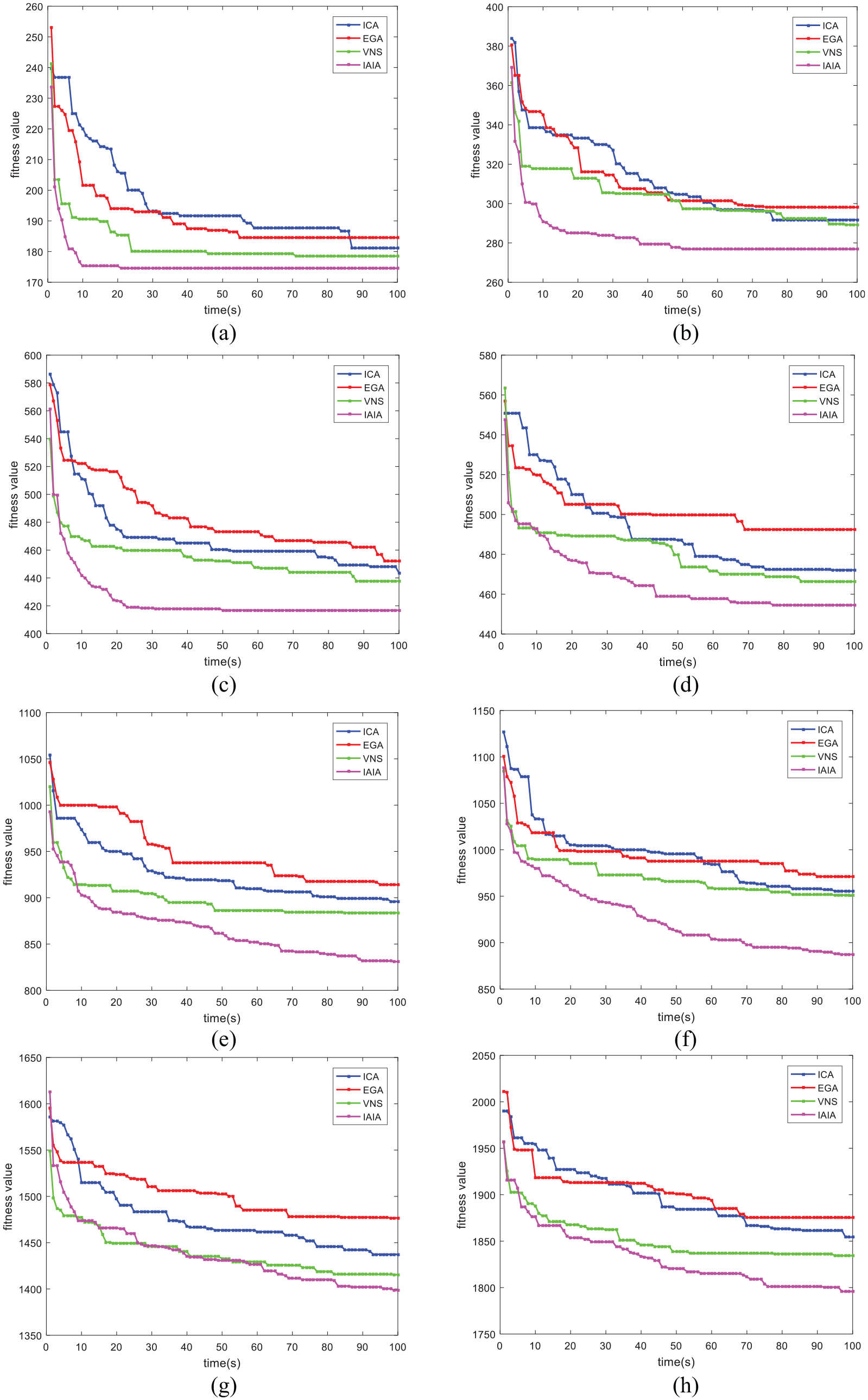
Convergence curve for instances under α = 0.8: (a) convergence curve for instance 10-5, (b) convergence curve for instance 10-8, (c) convergence curve for instance 20-6, (d) convergence curve for instance 30-5, (e) convergence curve for instance 30-10, (f) convergence curve for instance 50-7, (g) convergence curve for instance 50-10, and (h) convergence curve for instance 100-6.

Figure 9.

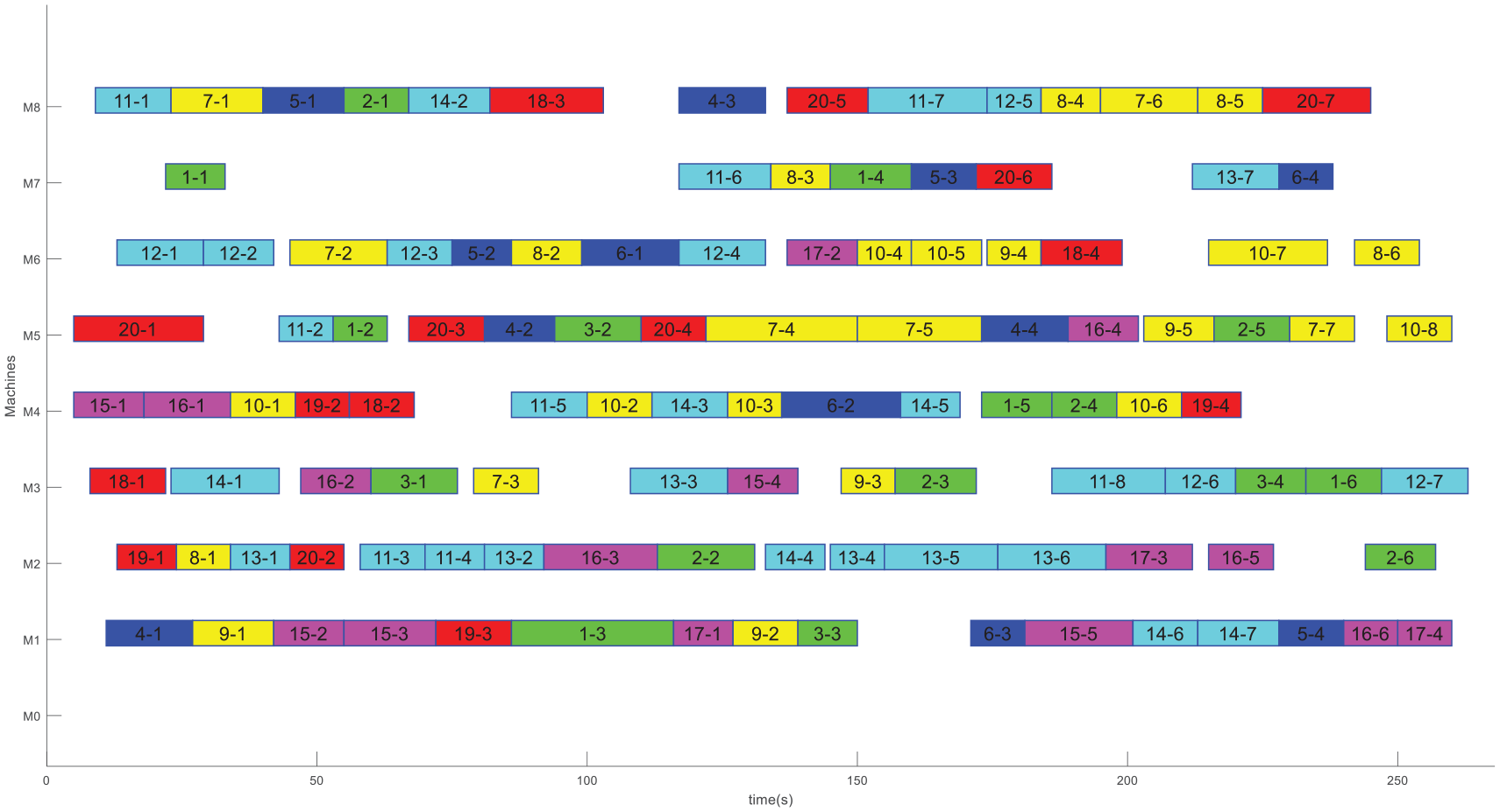
Gantt chart for instance 20-8 optimized using the IAIA.

We analyzed and summarized the reasons that the performance of the proposed algorithm is better than other three efficient algorithms as follows:

• (1) we applied three initial strategies to ensure that we can obtain effective solution, and these initial strategies do not require the repair mechanism.

• (2) the AIA is essentially an extension of the traditional GA and that not only has a powerful global search ability which but also improves the selection operator. To accelerate the convergence and avoid to fall in to local optimization, we introduced an operator of ERP that contains two parts, the calculation of fitness between antibodies and antigens, and the calculation of concentration between an antibody and other antibodies.

• (3) to avoid to fall into the local optimization, the SA algorithm is applied to local search in each neighborhood space of solutions.

In conclusion, the proposed algorithm achieved great improvement for optimizing the FJSP regardless of the solution accuracy and the computational time.

Conclusion and future research

Scheduling has always been one of the hot topics in manufacturing and production fields, and FJSP, as an extension of JSP, has received widespread attention because of its flexibility and realistic. In this study, we considered transportation time between machines, which are typically ignored in most literatures. We first modeled the FJSP with the transportation time as an extension of the canonical FJSP, denoting it as FJSP-T. Two objectives were considered simultaneously in the mathematical model, that is, the maximal completion time and the total energy consumption, and the weight decomposition is used to optimized the objectives. To solve this problem, a hybrid meta-heuristic algorithm based on the AIA and SA algorithm are proposed. In this algorithm, each solution is represented by two components, that is machine selection vector and operation sequence vector. Then, three initial strategies are applied to initial populations. To maintain the diversity of the population during iterations, an information entropy theory is embedded into the AIA for better global optimization. Meanwhile, the SA algorithm is proposed for further local search. Finally, a set of optimal parameters is obtained by using Taguchi method. To verify the validity of the FJSP-T model, the FJSP-T model is constructed by CPLEX, it is verified that the results obtained by CPLEX are not as good as that of proposed algorithm. In addition, we also carried out weight experiments under different coefficients, and analyzed the effectiveness of the algorithm under different coefficients. The multifactor ANOVA results and convergence curve comparisons also verified the competitiveness of the proposed algorithm. According to comparison with other meta-heuristic algorithms, the efficiency of the proposed algorithm is further proved.

However, there is still work to be considered in the future, we could (1) consider combining the flexible job shop scheduling problem with other complicated constraints that are typically ignored in this field to deploy our research to actual production, for example, fuzzy processing time, ⁴⁶ setup time, ⁴⁷ and distributed multi-factories ³⁶ ; (2) consider factors that we have not considered thoroughly enough, for example, the energy consumption generated by cranes in the process of handling and transferring, the energy consumption generated by machines in idle time ⁴⁸ ; (3) consider the normalization of multiple objectives ⁴⁹ ; (4) consider combining algorithms with neural model^50,51; and (5) consider applying the proposed algorithms to other scheduling fields.^52–54