
Abstract
Nonlinearities, uncertainties and external disturbances commonly exist in a wastewater treatment process (WWTP). Those issues present great challenges to the control of the dissolved oxygen (DO) concentration in a WWTP. In this paper, an active disturbance rejection control (ADRC) is utilized to estimate the total disturbance and drive the DO concentration to track the set-value. Simultaneously, an iterative learning strategy is employed to adjust the parameters of an extended state observer (ESO) to improve the accuracy of the estimation and reduce the dependence on experience in determining parameters. By combining the advantages of the ADRC and the iterative learning strategy, an iterative learning based active disturbance rejection control (ILADRC) is constructed, and the close-loop stability is analyzed. The benchmark simulation model No.1 (BSM1) is utilized to confirm the ILADRC. Numerical results show that the ILADRC is more effective in the DO concentration control.
Introduction
With the development of human society, freshwater becomes one of the most significant problems that we face due to the increasing demand and serious pollution. 1 The water crisis significantly affects several industries or even countries. 2 Therefore, the wastewater treatment attracts much attention. In early years, wastewater treatment processes (WWTPs) mainly relied on the manual control, the efficiency was low and the effluent quality could not satisfy higher effluent standards. 3 Thus, automatic control system has been applied in WWTPs.
Dissolved oxygen (DO) concentration directly affect the effluent quality, it has been commonly recognized as a key variable in a WWTP. Therefore, the control of DO concentration has been becoming a hot topic in the automatic control of a WWTP. However, kinds of control methods fail to regulate DO at a desired level due to WWTPs’ unique features, such as the varying rate of inflow, unstable compositions and concentrations, and unknown biochemical reactions, by comparison with other process industries.3,4 Much effort has been paid to address those challenges. PID control, a commonly used approach, has also been widely utilized in the DO concentration control. 5 However, the performance of the PID control degrades significantly for strong nonlinearities and disturbances in WWTPs. 5 To improve the tracking performance, a feedback linearization-based PI controller was designed. 6 Drawback of the feedback linearization method is that the robustness cannot be guaranteed for the existing uncertainties. 7 Nowadays, model predictive control (MPC) has a wide variety of applications. 8 In Zeng and Liu, 9 a centralized economic model predictive control (EMPC) was applied to a WWTP, the simulation results show that it can reduce operating cost and improve the effluent quality simultaneously. However, computational complexity resulting from solving the optimization problem and the relatively poor fault tolerance of a centralized control challenge its implementation. 10 Belchior 11 proposed a stable adaptive fuzzy control for a WWTP to control the DO. The algorithm achieved a promising result. However, traditional fuzzy control is largely dependent on input dimensions. If more input dimensions are defined, more fuzzy rules are necessary, and more computation complexity is involved. 12 In Bo and Zhang 13 an echo state networks based online adaptive dynamic programming was taken to control the DO concentration. Its design mainly depends on the online data, and minor prior knowledge is required.
It should be noted that the key point of the DO control in a WWTP is how to deal with the uncertainties, unknown dynamics, and disturbances. To estimate those undesired factors, various disturbance observer-based methods have been designed. Lin 14 proposed an adaptive neural control, it combined a nonlinear disturbance observer for a WWTP. Satisfactory performance was achieved. An active disturbance rejection control (ADRC) 15 was employed to control the DO concentration. The extended state observer (ESO) estimated the system states and total disturbance. Simulation results showed that the ADRC can achieve satisfied performance on DO concentration control. Based on the ESO, system can be dynamically transformed to be a linear system with connected integrators form. Then, a controller based on the idea of the U-model control is designed to control the DO concentration. 16 It does achieve faster and more robust response.
Actually, for the convenience in realizing, the effectiveness in dealing with strong disturbances and uncertainties, and the satisfied performance, ADRC has been applied in many fields.17–19 In this paper, we also focus on the ADRC. However, to some extent, determining parameters of an ESO depends on engineers’ experience. To make the ESO be more accurate in estimating and reducing the dependence on experience to fix the parameters, a P type iterative learning algorithm 20 is utilized, and the iterative learning based ADRC (ILADRC) 21 is designed in the DO concentration control. Main advantage of the ILADRC is that the ESO in the ILADRC can acquire better estimation performance by an iterative learning approach. Simultaneously, it reduces the requirement of an engineer’s experience.
The rest of this paper is organized as follows. Section II describes the model and control difficulties of a WWTP. Section III is controller design and stability analysis. Simulation results are shown in Section IV. Finally, a conclusion is drawn in Section V.
System description and control problem statement
System description
Benchmark simulation model no.1 (BSM1) is a benchmark simulation model for a WWTP. It contains influent data of dry, rain and storm weather, and it provides a set of standard evaluation criteria for different control strategies. 22 For fair comparisons among different control strategies, the BSM1 becomes a commonly accepted platform on benchmarking of control strategies for WWTPs. 22 Layout of the BSM1 is presented in Figure 1. 23 It consists of two parts. One is the biological reactor and the other is a secondary clarifier. The biological reactor comprises two anoxic tanks (V1=V2=1000 m3) and three aerobic tanks (V3 = V4 = V5 = 1333 m3). Biological and physical phenomena in tanks are described by activated sludge model no.1 (ASM1). The secondary clarifier is modeled as a 10 layers non-reactive unit.
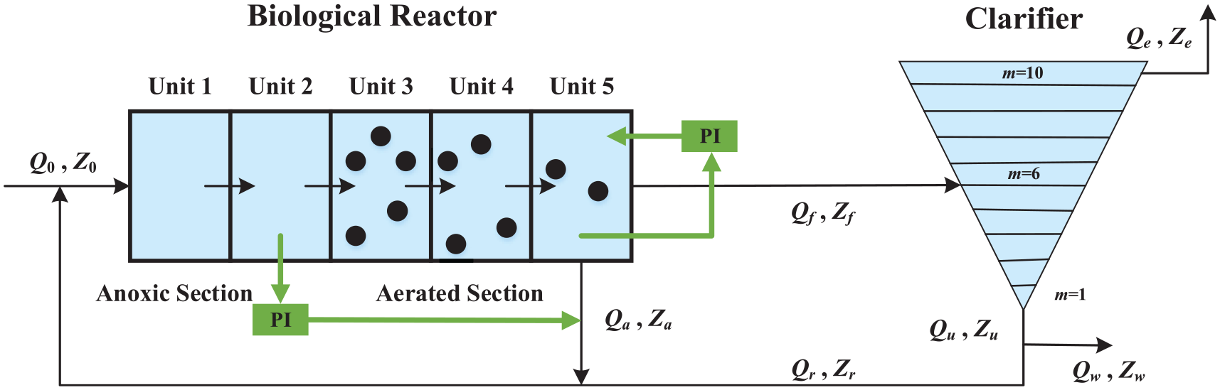
Layout of the BSM1.
Control problem statement
DO concentration in the fifth tank is a key parameter, which affects the growth of microorganisms and the effluent quality. Keeping it in a desirable level is critical for a WWTP. However, the DO concentration in the fifth tank is affected by various uncertainties, such as the time-varying influent components, concentrations, and inflow rates. Meanwhile, in practice, both parameters and dynamics of a WWTP are partially known or even completely unknown. Besides that, most issues are usually coupled with each other, and most of them are not available. In other words, disturbances, uncertain dynamics, and strong couplings are difficulties in keeping the DO concentration in a satisfied level. Thus, it is still a challenge to develop and apply an effective control strategy to satisfy the discharge requirements.
Therefore, the aim of this paper is to control the DO concentration in the fifth tank within a satisfied range by the oxygen transfer coefficient KLa5 in presence of disturbances, uncertain dynamics, and strong nonlinear couplings.
Iterative learning based active disturbance rejection control
Structure of the ILADRC
ADRC can estimate and cancel out the total disturbance in real time to guarantee the closed-loop system performance. Thus, an accurate mathematical model is not necessary. However, the parameters of an ESO determines its estimation ability greatly. To reduce the dependence on engineers’ experience in tuning parameters and improve ESO’s estimation ability, an iterative learning based ESO is designed. The structure of the ILADRC is given in Figure 2.
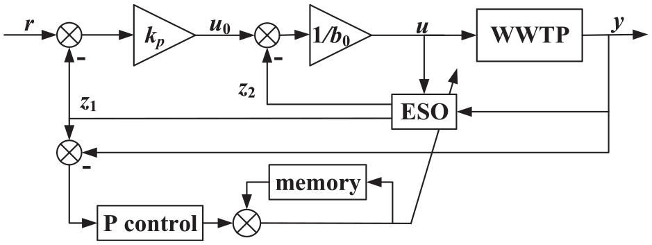
The ILADRC for a WWTP.
Here r is the set-value, u is the control signal, and y is the system output.
The ESO is designed as 24
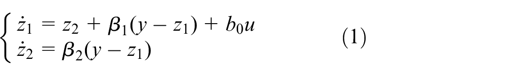
where b0, β1, β2 are adjustable gains of an ESO, y is the system output, u is the control signal, z1 is the estimation of y, and z2 is the estimation of the total disturbance.
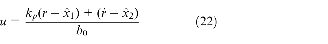
The control law is


where kp is an adjustable control gain.
In this paper, to decrease the estimation error of an ESO and reduce the dependence on experience in determining an ESO’s parameters, a P type iterative learning algorithm is utilized to adjust the parameters of an ESO, and it is designed as,


where k is the current iteration number,
According to the bandwidth-parameterization approach,
24
one has
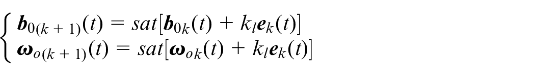
The bound of sat(·) should be chosen as large as possible to ensure the actually generated parameters would be within it. Then, we can say the generated parameters are always bounded. After the algorithm iterating n times, much smaller estimation errors can be obtained by the iterative learning based ESO.
Stability analysis
Consider a first-order system

where f represents the total disturbance, b0 is a non-zero constant, u is the control input, y is the controlled system output.
Let

where
Similarly, the ESO (1) can be rewritten as
where
Next, convergence of the iterative learning based ESO and the close-loop stability of ILADRC are analyzed.
Convergence of the iterative learning based ESO
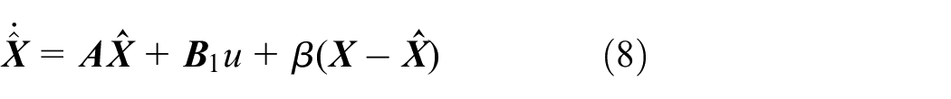
Subtracting equations (8) from (7), one has
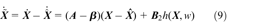
where
Let
where
Here,
Then, Theorem 1 is obtained.
Let
For j = 1,2, one has
For
System matrix
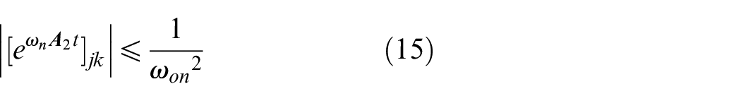
for all t≥T1, j, k = 1,2.
Thus
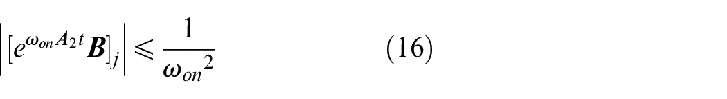
for all t≥T1.
Let
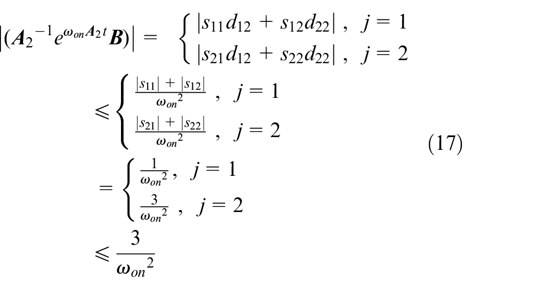
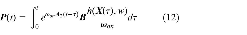
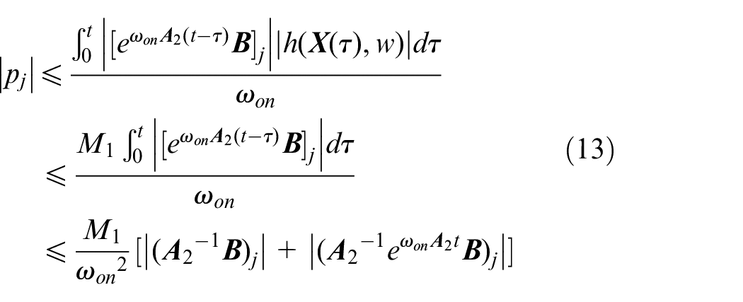
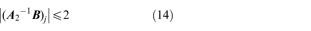
From equations (13), (14), and (17), one has
for all t≥T1, j = 1,2.
Let
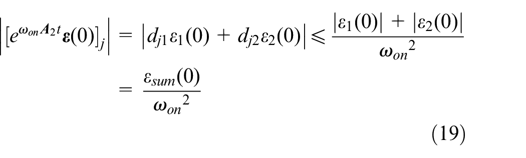
for all t≥T1, j = 1,2.
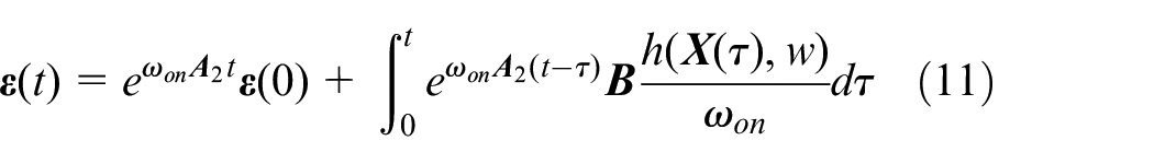
From equation (11), one has
Let
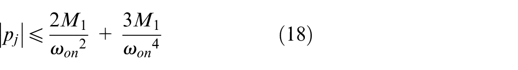
for all t≥T1, j = 1,2.
Thus, when h(
Close-loop stability of the ILADRC
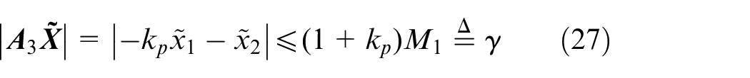
Control law of the ILADRC is
Substitute equations (22) into (6), one has

Let

Let

According to equation (25) and Theorem 1, one has
Let
Then
According to Gao,
24
one has
for all t≥T2.
Let T3 = max{T1, T2}, one has
for all t≥T3.
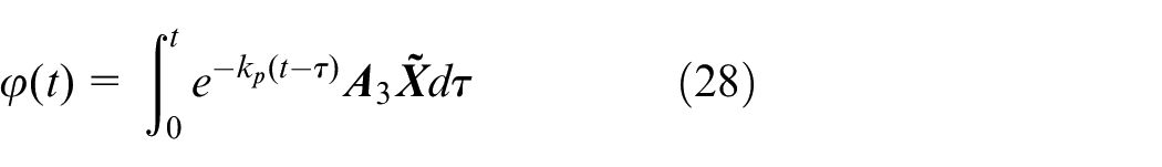
Then
for all t≥T3.
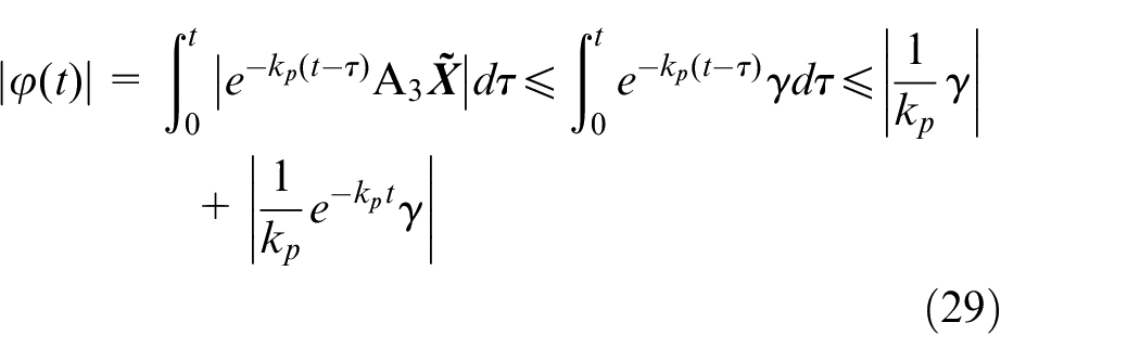
From equations (29) and (33), one has
for all t≥T3.
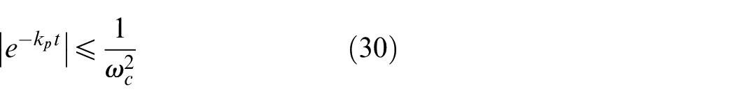
From equation (26), one has

Then,
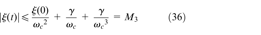
Based on Theorem 1 and Theorem 2, one can find that, if estimation errors of an ESO are bounded, tracking errors of the closed-loop system will also be bounded. Then, for a bounded set-value
Therefore, by choosing proper parameters, the iterative learning based ESO is bounded, and the closed-loop system is also stable.
Simulation results
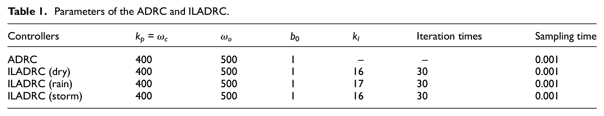
In this section, the iterative learning based ADRC is designed, and it is verified on the BSM1 under dry, rain and storm weather. The aim is to make the DO concentration in the fifth reactor (SO,5) at 2 mg/L by manipulating the oxygen transfer coefficient (KLa5). To confirm the ILADRC, the ADRC is taken to make a comparison. All experiments are based on the same numerical environments. Parameters of the ADRC and the ILADRC are listed in Table 1.
Parameters of the ADRC and ILADRC.
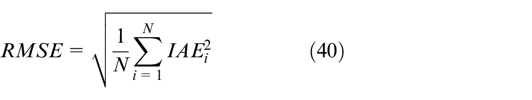
The performance is evaluated by the integral of absolute error (IAE), integral of squared error (ISE) and the maximal deviation from the set-value (DEV max ). IAE, ISE, and DEV max can be calculated as 22
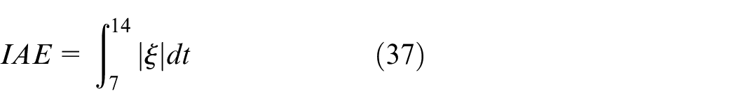
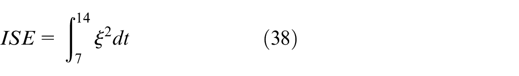

where
For the ILADRC, in each experiment, initial learning gain kl is determined by try and error, and they are listed in Table 1. To obtain a better learning gain, Monte Carlo experiments are carried out. To ensure the learning gains kl s in Monte Carlo experiments are selected properly, they randomly vary in ±20% of their initial values. In other words, in dry and stormy days
Based on kl s, bandwidths ωos and b0s of the ILADRC can be obtained. The ωos and b0s after 30 times iterations are listed in Table 2. Other parameters are the same with those given in Table 1.
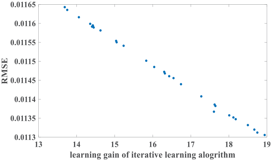
Learning gains (kl s) and RMSEs in dry weather.
Main parameters of the ILADRC after 30 times iterations.
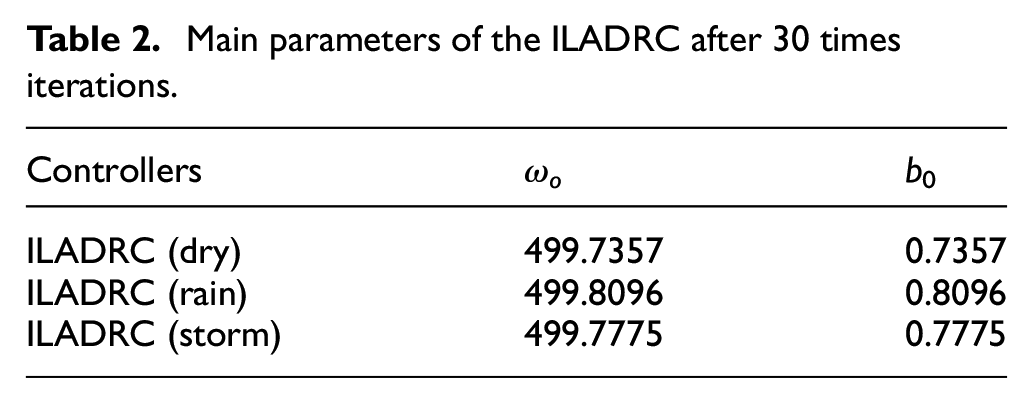
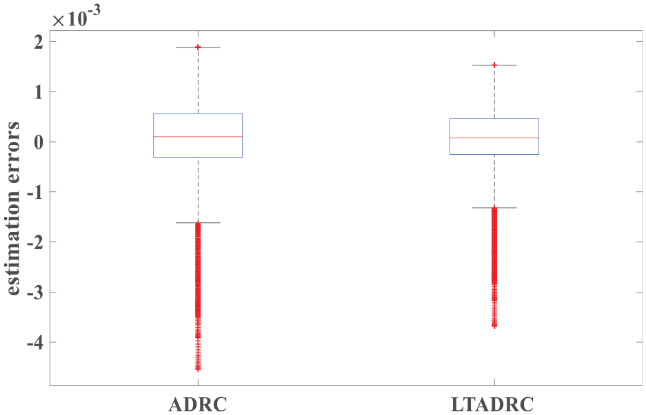
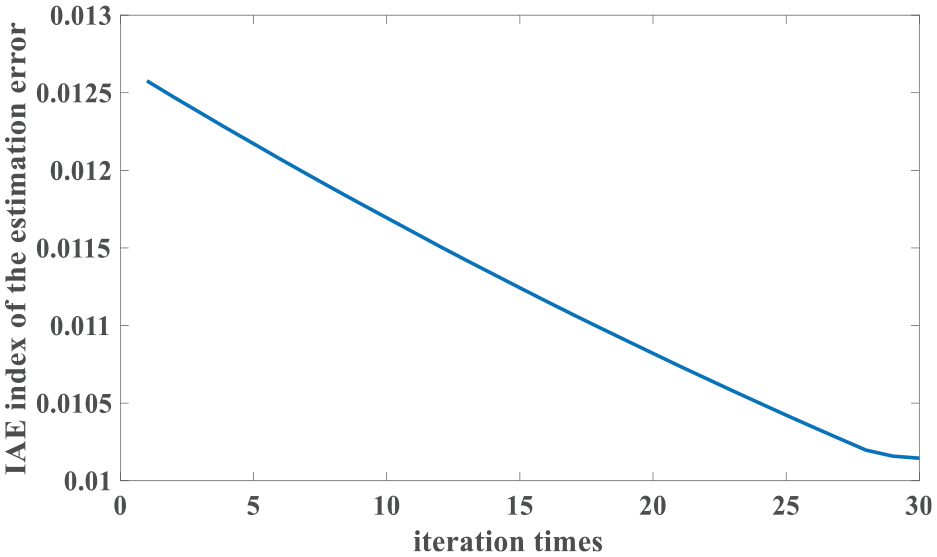
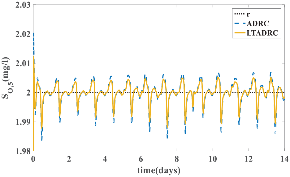
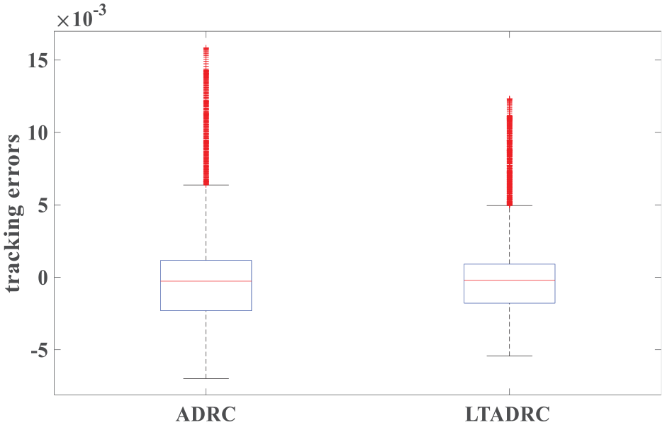
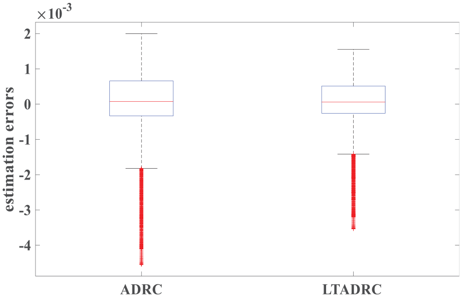
Figure 4 shows the tendency of IAE values when kl = 19.0118. In this case, outputs of the ILADRC are given in Figure 5. Simultaneously, outputs of the ADRC are also shown in Figure 5. From Figure 5, it is easy to find that the ILADRC achieves better tracking performance in dry days. Figures 6 and 7 are tracking errors and estimation errors of the ADRC and the ILADRC. The median of both tracking error and estimation error equal zero, it means the average level of those errors is zero. The distance of upper and lower quartiles in the boxplot reflects the varying degree of the tracking and/or estimation errors. Higher the boxplot, larger fluctuations of the errors. Figures 6 and 7 show that, by comparison with the ADRC, both tracking errors and estimation errors of the ILADRC have fewer changes and closer to the median. Fewer outliers of the ILADRC also means ILADRC is more effective. Performance values listed in Table 3 confirm the fact discussed above in a quantitative way.
IAE values in dry weather (kl = 19.0118).
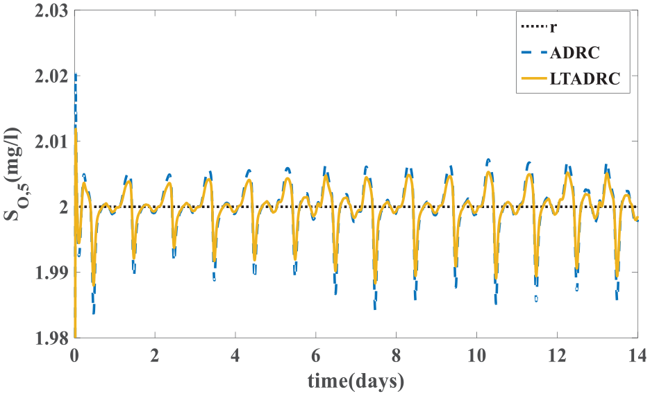
Tracking performance in dry weather (kl = 19.0118).
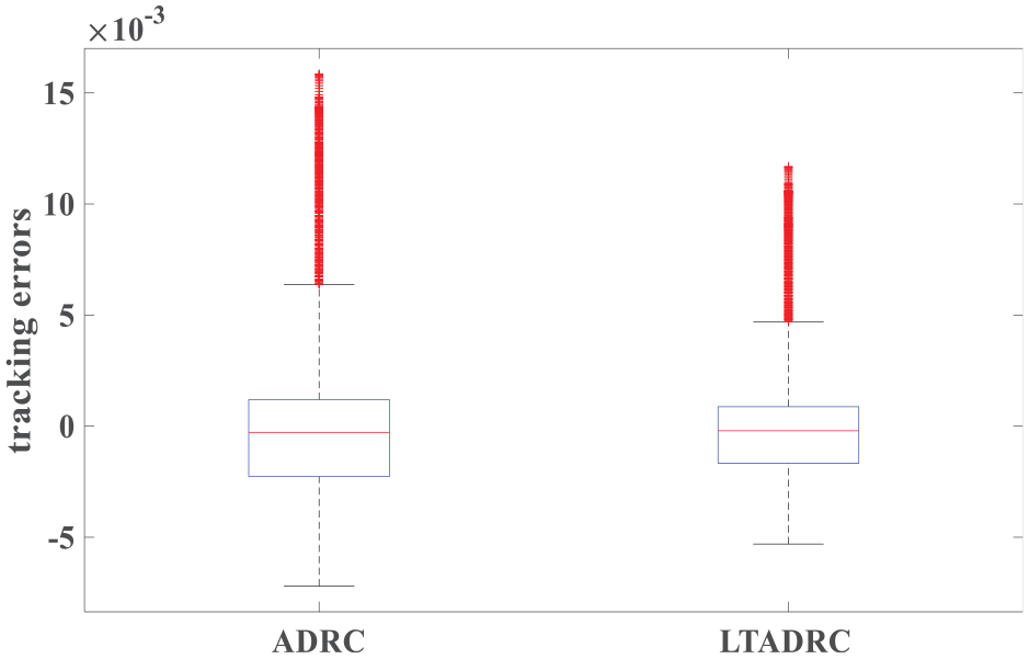
Tracking errors of the ADRC and the ILADRC in dry weather (kl = 19.0118).
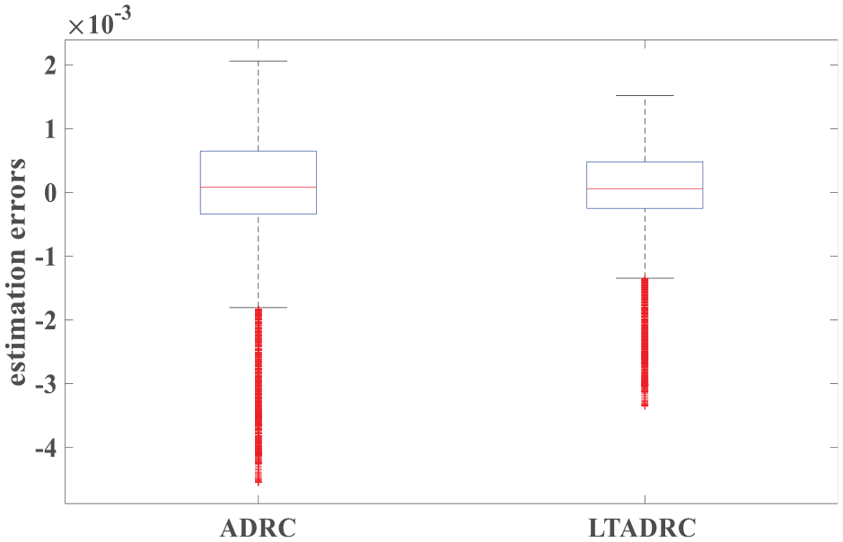
Estimation errors of the ADRC and the ILADRC in dry weather (kl = 19.0118).
Performance values of the ILADRC and the ADRC.
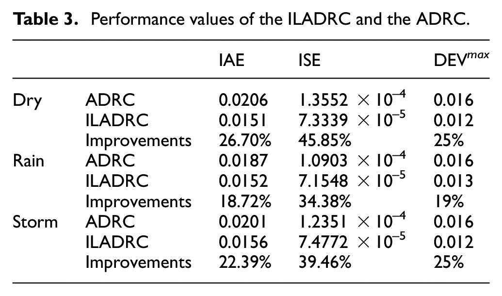
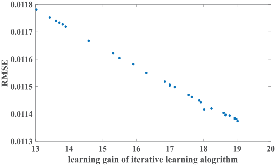
Figure 8 shows the relationship between the learning gains (kl s) and RMSEs. It can be found that, when the learning gain kl = 20.2000, the RMSE value is minimum.
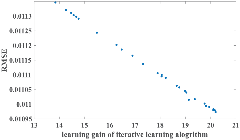
Learning gains (kl s) and RMSEs in rain weather.
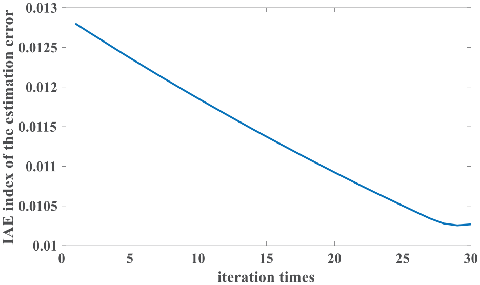
Figure 9 presents the IAE values of the estimation errors. System outputs of the ADRC and the ILADRC are shown in Figure 10. From Figure 10, it is easy to see that better tracking performance is obtained by the ILADRC in rain weather. Figures 11 and 12 are tracking errors and estimation errors of the ADRC and the ILADRC. Both tracking and estimation errors of the ILADRC are smaller than the ones of the ADRC. Performance values are shown in Table 3.
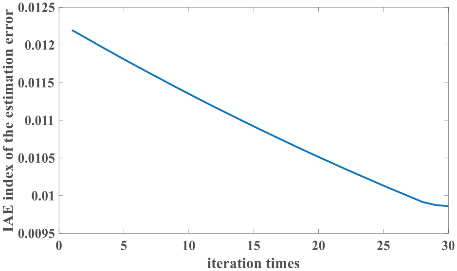
IAE values in rain weather (kl = 20.2000).
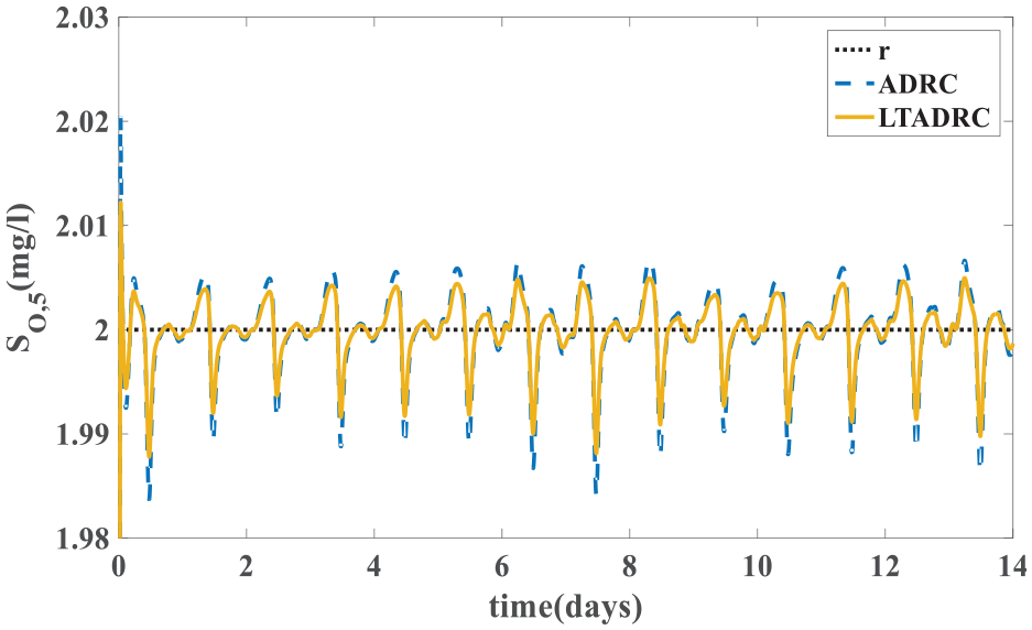
Tracking performance in rain weather (kl = 20.2000).
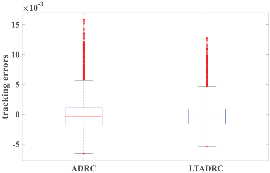
Tracking errors of the ADRC and the ILADRC in rain weather (kl = 20.2000).
Estimation errors of the ADRC and the ILADRC in rain weather (kl = 20.2000).
Figure 13 shows the relationship between learning gains (kl s) and RMSEs in stormy days. When kl = 18.9395, RMSE is minimum.
Learning gains (kl s) and RMSEs in storm weather.
Figure 14 is the IAE values of the estimation errors. It illustrates that the learning process is convergent. System outputs of the ADRC and the ILADRC are shown in Figure 15. It indicates that ILADRC has better tracking performance. Figures 16 and 17 show that the average level of the tracking errors and estimation errors are close to zero. In addition, from the distance of upper and lower quartiles in boxplots, one can see that the tracking errors and estimation errors of the ILADRC system are closer to zero. Performance comparisons in storm weather are also given in Table 3.
IAE values in storm weather (kl = 18.9395).
Tracking performance in storm weather (kl = 18.9395).
Tracking errors of the ADRC and the ILADRC in storm weather (kl = 18.9395).
Estimation errors of the ADRC and the ILADRC in storm weather (kl = 18.9395).
In Table 3, the improvements signify that the ILADRC is superior to the ADRC from the perspective of IAE, ISE and DEV max . For example, in dry days, ISE values of the ILADRC are improved by 45.85% by comparison with the ADRC. Data listed in Table 3 confirm the advantage of the iterative learning based ESO.
From the simulation results in dry, rain and storm weather, it is obvious that, because of an iterative learning ESO, the ILADRC tracks the set-value more accurately. It demonstrates that, compared with a conventional ESO, an iterative learning ESO can estimate the total disturbance more effectively. Simultaneously, when choosing the parameters, the iterative learning based ESO is less dependent on the experience of an engineer. It helps improve the estimation and control performance of the ADRC.
Conclusion
A WWTP is a time-varying system with strong nonlinearities and couplings. In addition, kinds of uncertainties and disturbances are also existing. Therefore, it is impossible to establish an accurate model for the control of a WWTP. In this paper, an iterative learning based ADRC is designed for the DO control in a WWTP. The iterative learning method is utilized to optimize the parameters of an ESO. Compared with the conventional ESO whose parameters are fixed, the iterative learning based ESO achieves a more accurate estimation. Then, the close-loop DO concentration control of a WWTP is more satisfied. Advantages of the iterative learning based ESO and the ILADRC show that it may be a promising way to control the DO in a WWTP. However, it should be verified in a real wastewater treatment process and it is our future work.
Footnotes
Declaration of conflicting interests
The author(s) declared no potential conflicts of interest with respect to the research, authorship, and/or publication of this article.
Funding
The author(s) disclosed receipt of the following financial support for the research, authorship, and/or publication of this article: This research is supported by Key program of Beijing Municipal Education Commission (grant no.: KZ20181 0011012) and National Natural Science Foundation of China (grant no.: 61873005).