Sage Journals: Discover world-class research

Abstract

The major concern in the high tech industries like oil and petroleum industries, automobiles, aeronautical, and nuclear power plants is the control of the defects like distortion in the welded joints and residual stresses occur due to arc welding on the circumferential joints of the thin pipes. Three-dimensional non-linear thermal and thermomechanical numerical simulations are conducted for the tungsten inert gas welding process of SS-304 stainless steel pipes. In this article, numerical analysis of the distribution of the temperature and the welding residual stress fields induced after the welding is done. Study on the effect of the welding heat input by varying the welding parameters (like welding current and welding speed) based on finite element simulations is conduit to examine the results on the residual stresses which is also called as the ‘locked-in’ stresses. The precision of the finite element model is validated for the welding residual stresses. The intention of this study is to provide the information to verify the validity of ongoing process circumferential manufacturing technology for thin-walled pipes, so to avoid the failure of these kinds of structures which are in service because of these intrinsic stresses.

Keywords

Heat input residual stresses stainless steel tungsten inert gas welding

Introduction

Thin welded pipes are generally used in a variety of engineering applications like pressurized piping system, thermal and nuclear power plants, and petroleum industries. The failure of these kinds of structures is due to the decrease in the strength in and in the region of the weld area of the arc welding process, and the main apprehension of the welding industry is residual stresses. The concerned area of the residual stresses is where there is gradual change in the temperature due to the rapid heating and cooling during the welding, which is near the weld bead. During the heating phase, the strain produced always induces the plastic deformation of the metal. These strains which result the stresses produce the forces that cause the different types of welding distortion. Welding residual stresses and welding distortion play a vital role in the reliable design of the welded structure and joints. The reason of the main problems like stress corrosion cracking, damage due to fatigue, and brittle fracture is only the tensile welding residual stresses. This is the reason it become necessary to precisely predict and manage residual stresses in arc welding processes.¹

As the welding process is very complex, it becomes difficult to precisely predict the welding residual stresses. Numerical simulation based upon finite element (FE) technique is a proven helpful tool to capture the accurate temperature distribution and the welding residual stresses in welding technology. As of late, FE modelling have turned into an amazing asset for the calculation of defects which are due to the welding like stresses induced into the material and deformation of the structure. An important work on the numerical analysis and experimentation of thin pipe welding has been reported by researchers.²

In the course of the most recent two decades, various FE numerical models have created to foresee weld-induced stresses and simulation of the circumferential welding on the butt joint pipes. Varma Prasad et al.³ studied on the various welding parameters to see the effect on the welding residual stress and distortion in the stainless steel welded pipes. The effect of the different clamping condition on the welding residual stresses was determined and concluded that the clamping of the work piece resulted in the more welding residual stresses.⁴ With the change in the orientation of the welding, there is great change in the welding distortion.⁵ Simulation of the submerged arc welding process was done using the commercial software ANSYS. The temperature distribution and the angular displacement of the mild steel welded plate were compared with the experimental data of Arora et al.⁶ and found the good agreement with conclusion that the double-ellipsoidal heat source is more accurate than the Gaussian heat source distribution.⁷ They represented the computational analysis of the welding distortion and welding stresses induced by the submerged arc welding process. This was done by using the ANSYS FE software. The non-linear problem was found in the welded distorted plate in material and geometry, which result in the FE solution based upon the thermo-elasto-plastic theory.⁸ Presented the numerical approach to determine the temperature field and the locked in stresses in the stainless steel SUS304, multi-pass welded pipe using the ABAQUS software. Both three-dimensional (3D) and two-dimensional (2D) models were developed which were engaged to measure the temperature profile and the stresses fields. The 2D axisymmetric model was developed on the basis of characteristics of the temperature field and the locked in stresses. The simulation results of the 2D model were found effective, and it can be used for the simulation of the temperature profile and residual stress fields for the SS pipes. With the 2D model much time can be saved as reported by Akbari Mousavi and Miresmaeili.⁹ Numerical simulation of temperature distribution and welding residual stresses due to the welding process was done by using the ANSYS code. They found the effect of the welding current and the effect of varying the thickness on the residual stresses. After the welding in the cooling phase, there is shrinkage and deformation in the weld zone, which leads to the compressive and the tensile residual stresses on the outer and the inner zones, respectively.¹⁰ The effect of various boundary conditions on the welding locked in stress fields is studied. The consequences of the boundary condition on controlling the welding locked in stresses were discussed, and the less dependency of structural constraints on the welding locked in stresses was found. The magnitude of the stresses varied with the different boundary conditions but the pattern remains the same.¹¹ A numerical approach of tungsten inert gas (TIG) welding simulation on the basis of 3D model to accurately predict the temperature and weld-induced stresses is presented. The nature of the stresses is predicted as the compressive and tensile on or near the weld line and away from the weld line, respectively. Tensile and compressive stresses are off from the weld centre line on the outer and inner surfaces, respectively.¹² The consequence of the boundary condition on the welding locked in stresses was compared, and it was found that there is a minute effect of the boundary condition on the welding locked in stresses. They concluded that the welding residual stresses in the free plate have very less residual stresses as compared to the plates of the large structure or have displacement constraint.¹³ They analysed the consequences of the various different welding sequences on the temperature and locked in stresses induced in the welded pipe. Results showed that except the starting location, there is no effective difference in the axial and hoop residual stresses in the welded pipe.¹⁴ Computational procedure is proposed by the Hwang et al.¹⁵ in which the residual stresses in the welded T-joint are measured using the X-ray diffraction (XRD). The 3D FE analysis was done to find out the profile of the residual stresses, and the proposed model was validated with the experimental result. Residual stresses were analysed using the 2D and 3D models produced in the TIG welding process. The effect of geometry configurations on the residual stress distributions is predicted from the 3D computer analysis using a thermo-elasto-plastic constitutive equation and compared with the XRD method.9 The residual stresses in weldments of nickel-based superalloy Inconel 625 and stainless steel 316L using continuous current gas tungsten arc welding (CCGTAW) and pulsed current gas tungsten arc welding (PCGTAW) process employing ERNiCrMo-3 and ERNiCr-3 fillers are evaluated.¹⁶ The welding-induced residual stresses in steel plates due to multi-pass welding are investigated numerically and experimentally. The transient FE model is developed to estimate the axial residual stresses induced by butt welding. Element birth and death technique is used to simulate the welding process in ANSYS. The XRD method is used for measuring the residual stress. A good agreement is achieved between numerical and experimental results. It is concluded that multi-pass welding has significant effects on the residual stress distribution.¹⁷ The formation behaviour of welding residual stresses during the circumferential TIG butt welding of pipes is analysed. A 3D thermo-elasto-plastic numerical model has been developed by using MSC-Marc software to predict welding residual stress distributions during single-pass welding of pipes.1 The effect of the residual stresses on the fatigue crack growth on the weldment of stainless steel grade SS-316L was studied.¹⁸ Submerged arc welding of SA 516 grade 60 pressure vessel grade steel was conducted with different heat plate thicknesses, and the influence of cooling rate on microstructure, Vickers hardness, and impact toughness of heat-affected zone (HAZ) of weldment was systematically investigated.¹⁹ Chujutalli and Estefen²⁰ proposed a method to estimate the heat source parameters, which combines analytical formulation, experimental data, and numerical simulations. The effect of the welding parameters on the welding residual stresses in circumferential TIG welding process was found by Varma Prasad et al.3 The 3D numerical simulation ANSYS code is used to predict the residual stress distribution developed during circumferential TIG welding. Welding simulation of a stiffened plate structure with longitudinal and transverse stiffeners using a thermo-elasto-plastic FE method was done by Chen and Shenoi.²¹ A 3D thermo-elasto-plastic FE analysis was used to determine the residual stress distribution and the distortion field in butt and fillet plates. The FE model was employed, which was first verified against existing experimental results of thermal distortion and then was used for analysing 12 case studies accounting for various plate thicknesses and welding sequences.²² Employing the FE method, the butt-weld-induced thermal field and distortion of steel plates were analysed, and the effect of the welding sequences was studied.²³

Many researchers predicted the residual stresses on the welded plates; in this article, for the prediction of the welding residual stresses during the single-pass circumferential welded pipes, a thermo-mechanical 3D FE model has been developed using the FE software MSC-Marc. The precision of the developed model is verified from the experimentally measured longitudinal and hoop stresses. At that point, utilizing a numerical computational methodology, we confirmed the method of the adjustments in weld-induced locked-in stresses and deformation all through the welding procedure to investigate the pattern of the stresses in thin circumferential welded pipes. In addition to this, the effect of the welding heat input on the welding residual stresses has been determined. Finally, there is a sensible clarification to the trend of the hoop and the axial residual stresses in and around the weld bead area of the welded pipe.

FE simulation

In this FE simulation, a numerical model which is a thermal–mechanical model has been formulated utilizing the MSC-Marc software to get the thermal profile at the nodes and the weld-induced stresses in the TIG circular welded butt joint pipes. The arrangement method comprises two stages. To start with, the temperature profile and the transient thermal cycle are calculated using the transient thermal analysis. After getting the thermal results, the results are utilized as the thermal load in the structural analysis to get the structural results in terms of the weld-induced stresses.

FE model

For thin pipes, a single-pass circumferential welded butt joint FE model is developed as shown in Figure 1. The pipe used in the model is stainless steel Sch5S having inside diameter of 80 mm and thickness of 2.11 mm. The length of one part of the pipe is 100 mm. Meshing on and near the weld centre line is relatively fine as compared to the area away from the weld line, as on and near the weld line there is rapid change in temperature, which results in stress gradients in weld bead and in HAZ.²⁴ The element type in the thermal analysis is Quadrilateral 4 having one degree of freedom (DOF) that is temperature and the type of the element in the structural analysis is Quadrilateral 4 having 3 DOF of translation in x, y, and z directions. The element size in the transverse direction to the weld bead in the area of weld bead and the HAZ is 0.25 mm, which will give you the accurate data, but it takes little much time as the number of nodes and element increase with decrease in the size of element. The element size increases as moving away from the weld bead. The element size along the weld direction is 2.55 mm which is constant.²⁵ In the direction of thickness, the number of elements is 5. With the increase in the element number, the direction of thickness remains the same, so keeping the element number low saves the computational time. The pipe material is stainless steel SS-304 whose thermostructural properties are shown in Figure 2. The properties of the material are extracted from the JMatPro software in which spectrograph report is utilized as input to get the properties (like modulus of elasticity, thermal conductivity, and yield strength).²⁶

Figure 1.

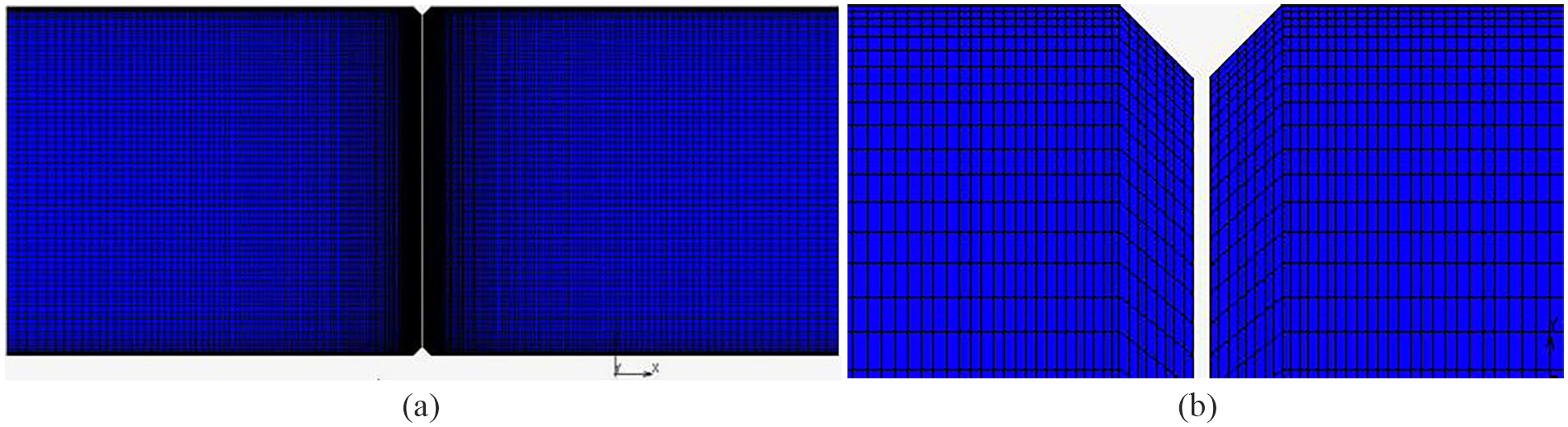
(a) The model of the pipe with meshing and (b) the V groove with root opening.

Figure 2.

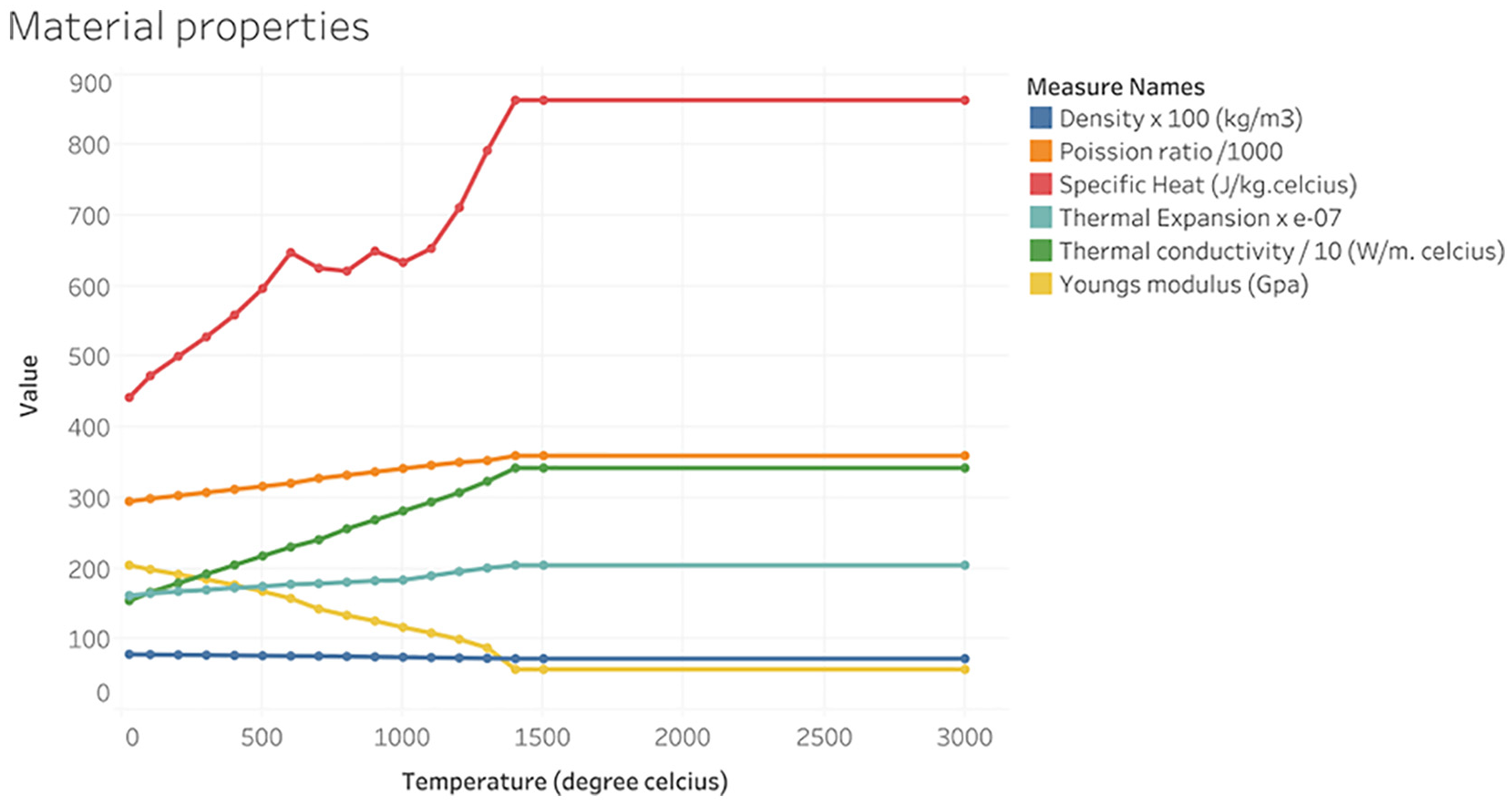
Temperature-dependent properties of the SS-304 stainless steel.

Thermal analysis

The temperature around the welded area should be in certain limits to manage the metallographic changes; stresses produced due to the welding and deformation of the structure, which are outcomes of a welding process.

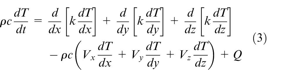
Due to change in the temperature field, the locked-in stresses generate in the welded structures. The travelling of heat in the welded structure is mainly due to the conduction of the heat which is articulated by the heat flow equation as follows¹⁰

\begin{matrix} ρ c \frac{dT}{dt} = \frac{d q_{x}}{dx} + \frac{d q_{y}}{dy} + \frac{d q_{z}}{dz} \\ - ρ c (V_{x} \frac{dT}{dx} + V_{y} \frac{dT}{dy} + V_{z} \frac{dT}{dz}) + Q \end{matrix}

(1)

q_{i} = k \frac{dT}{di}

(2)

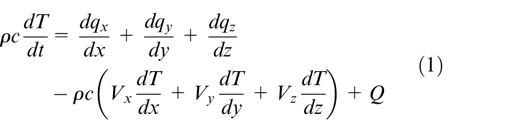
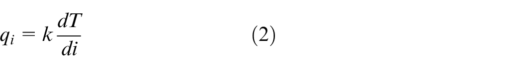
where i is the coordinates x, y, and z of the isotropic media and i = x, y, and z. Replacement of Fourier’s law relations (2) in equation (1) gives the heat transfer equation as follows²⁷

\begin{matrix} ρ c \frac{dT}{dt} = \frac{d}{dx} [k \frac{dT}{dx}] + \frac{d}{dy} [k \frac{dT}{dy}] + \frac{d}{dz} [k \frac{dT}{dz}] \\ - ρ c (V_{x} \frac{dT}{dx} + V_{y} \frac{dT}{dy} + V_{z} \frac{dT}{dz}) + Q \end{matrix}

(3)

For thermal analysis, a double-ellipsoidal model is used as the heat source model.²⁸ The power density distribution of this model for front and rear quadrants, respectively, when expressed in Cartesian coordinate system (x, y, and z) is reproduced as follows

q_{f} (x, y, z) = \frac{6 \sqrt{3} f_{f} Q}{ab c_{f} π \sqrt π} . e^{- 3 \frac{x^{2}}{a^{2}}} . e^{- 3 \frac{y^{2}}{b^{2}}} . e^{- 3 \frac{z^{2}}{c_{f}^{2}}}

(4)

q_{r} (x, y, z) = \frac{6 \sqrt{3} f_{r} Q}{ab c_{r} π \sqrt π} . e^{- 3 \frac{x^{2}}{a^{2}}} . e^{- 3 \frac{y^{2}}{b^{2}}} . e^{- 3 \frac{z^{2}}{c_{r}^{2}}}

(5)

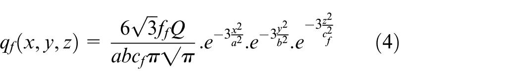
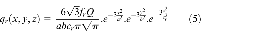
where Q = ηVI is the power input of the heat source of welding. The ellipsoidal parameters a and b are same for the front and rear quadrants, whereas parameter ‘c’ has different values defining the front ellipsoid (c_f) and rear ellipsoid (c_r). The parameters f_f and f_r define the fraction of total heat in the front quadrant and rear quadrants, respectively, with f_f + f_r = 2.0. The power of the heat source is denoted by Q which is the product of current, voltage, and arc efficiency²⁹

Q = η VI

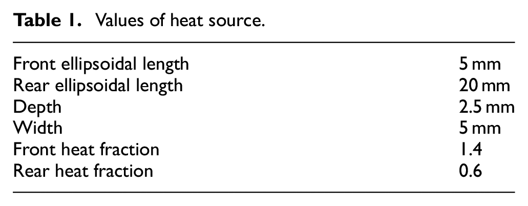
The arc efficiency of the TIG welding process is assumed as 75% to compensate for unaccounted losses. Values of all the parameters defining double-ellipsoidal heat source distribution are given in Table 1¹¹ in combination with the parameters of the welding process which were validated with the experimental data in this study.

Table 1.

Values of heat source.

Front ellipsoidal length	5 mm
Rear ellipsoidal length	20 mm
Depth	2.5 mm
Width	5 mm
Front heat fraction	1.4
Rear heat fraction	0.6

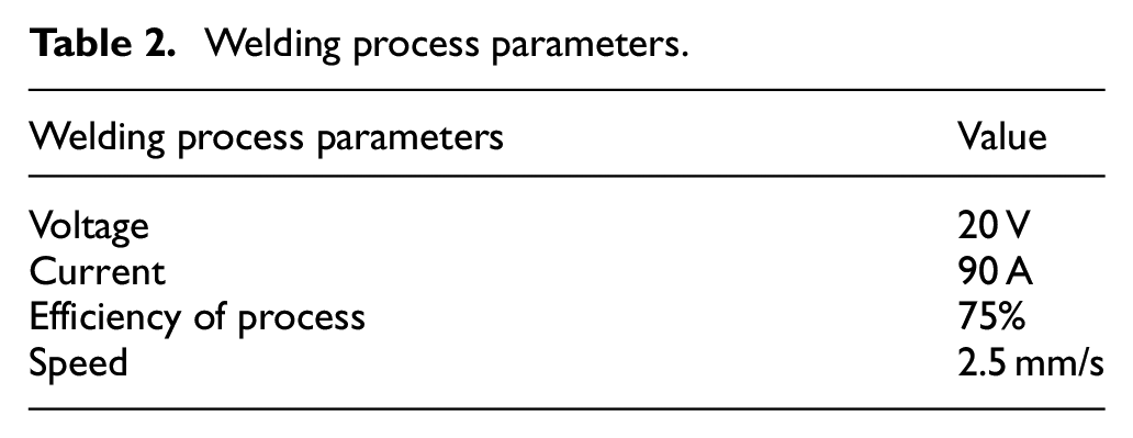
The heat source parameters are selected on the basis of the geometry of the weld bead; these are the parameters which define the structure of the weld bead according to the conditions of welding. The welding parameters are shown in Table 2.

Table 2.

Welding process parameters.

Welding process parameters	Value
Voltage	20 V
Current	90 A
Efficiency of process	75%
Speed	2.5 mm/s

All through the process of TIG welding, radiation and thermal convection were considered for the loss of heat. Losses due to the radiation are prevailing at high temperature on the selected area that is weld bead, and convection loss prevails at lower temperature on the area adjoining to the weld bead.³⁰ In this manner, both the heat losses are considered for the analysis of the pipe welding. The combined heat loss coefficient can be determined by using the following equations³¹

Q (loss) = q (convection) + q (radiation)

(6)

H (total) = 0.067 (W / m^{2}) 0 < T < 500 ° C

(7)

H (total) = 0.23 T - 82 (W / m^{2}) T \geq 500 ° C

(8)

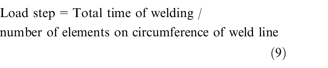
The technique which was used earlier that is quiet element which is easy to put into practice in the MSC-Marc in the present study property of element birth and death technique are inserted in which the filler will be inserted as the arc moves as the conductivity increase. The whole model is developed in the beginning with the filler metal, and all elements are deactivated in the starting by assigning low conductivity.³² In the investigation, the temperature of all the nodes is fixed at ambient temperature till the birth of element which comes under the arc. Dead elements are regenerated in sequence when they approach beneath the welding arc. For the accurate results, the welding arc should be present minimum one time on every element along the weld centre line. Minimum criteria for the selection of the load step are given in equation (9)³³

\begin{array}{l} Load step = Total time of welding/ \\ number of elements on circumference of weld line \end{array}

(9)

Mechanical analysis

The structural investigations are directed with the help of thermal profile which was calculated with the preceding thermal analysis procedure for every step increment for the prediction of the welding stresses. In conjunction with the structural boundary conditions, the mechanical properties are incorporated as shown in Figure 2.

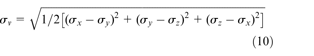
Thermal–structural material detailing as appeared by equation (10) with von Mises yield criteria is utilized with $σ_{x}$ , $σ_{y}$ , and $σ_{z}$ being the stresses, coupled to a kinematic hardening rule³⁴

σ_{v} = \sqrt{1 / 2 [{(σ_{x} - σ_{y})}^{2} + {(σ_{y} - σ_{z})}^{2} + {(σ_{z} - σ_{x})}^{2}]}

(10)

The number of nodes and elements were taken as same in the thermal analysis for the mapping of nodes and elements with the same topology to upgrade the junction in the mechanical analysis.

In the analysis, the constraint in the y and z directions is applied on the one side of the cylindrical pipe to validate the experimental condition as shown in Figure 3. Nodes at the end of the pipe on a Cartesian coordinate axis are selected and constrained to move in the transverse direction.²⁷ For the study of the parameters, the constraint condition is shown in Figure 3. The nodes at the end of both sides of cylindrical pipes are selected and translation movement in all the directions is fixed.

Figure 3.

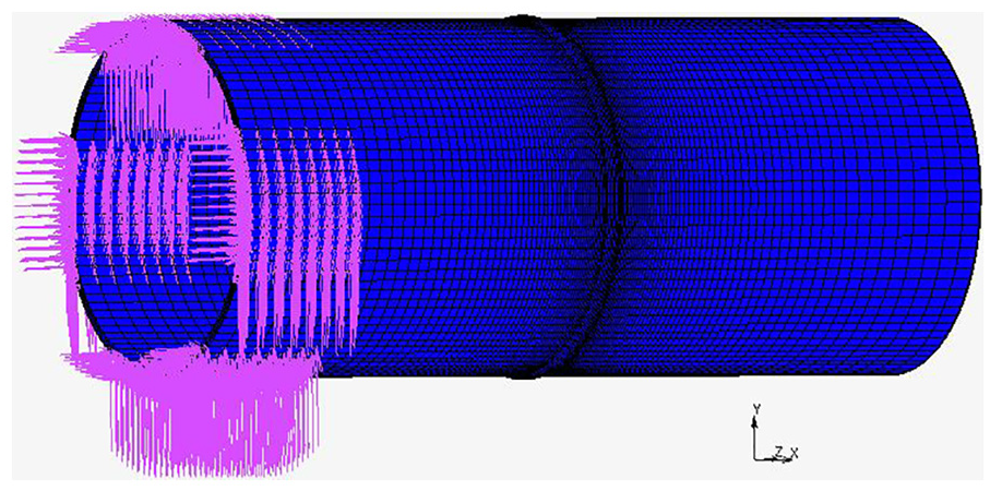
The structural boundary condition.

Validation of the model

Experimental procedure

In this study, to make sure the developed FE model is reliable, TIG welding on the SS-304 pipe having same geometrical parameters and welding parameters as listed in Table 2 from the model was conducted. Pipe is welded with the single pass having ‘V’ groove and 1 mm root opening. The axial residual stresses were calculated by FE model and compared with the experiments done in workshop.³⁵ Automated welding fixture was manufactured for least human involvement, and it is required for the correct validation of the model as shown in Figure 4. It was observed that the FE model results are in decent agreement with the experimental data. This whole indicates that the developed FE model using the commercialized software MSC-Marc can be used in industries for the calculation of the residual stresses in the welded structure without the experiments by which we can save lot of money and labour.³⁶

Figure 4.

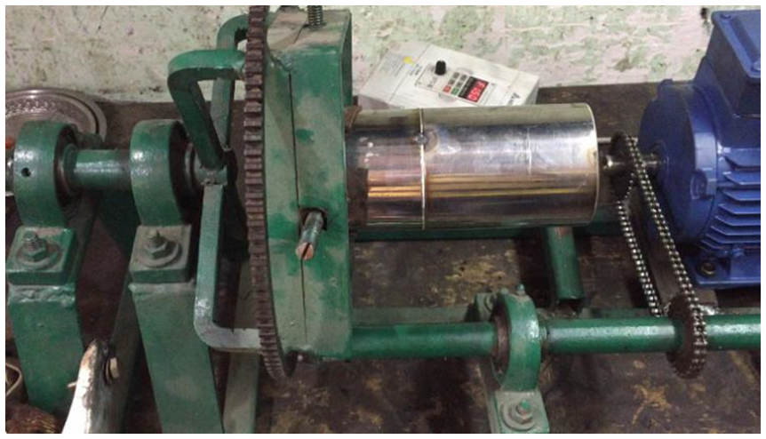
The rotational jig for welding with constant speed.

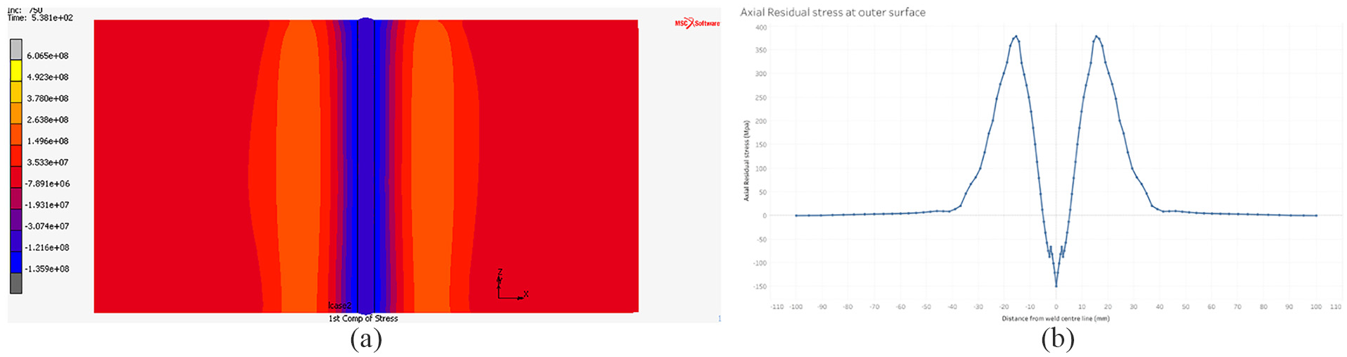
Figure 5 shows the contour plot of residual stress, which shows that on the outer surface of the weld bead there is compressive stresses around −90 MPa, and the magnitude and the type of the axial residual stresses near the weld bead in the HAZ are changed to tensile around 55 MPa. The axial residual stresses around 5–15 mm from the weld bead change the nature of the stress to tensile and the magnitude of the stresses is around 55–324 MPa. Figure 6 shows the curve of the axial residual stress compared with the experimental data of residual stresses measured with the XRD.³⁷

Figure 5.

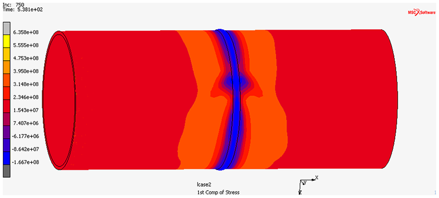
The contour plot of residual stresses.

Figure 6.

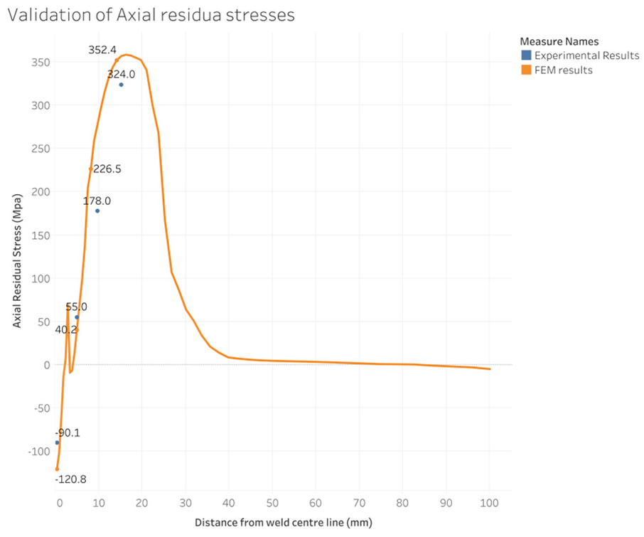
The axial residual stresses predicted by FEM and compared with the experimental data.

Results and discussion

Thermal analysis

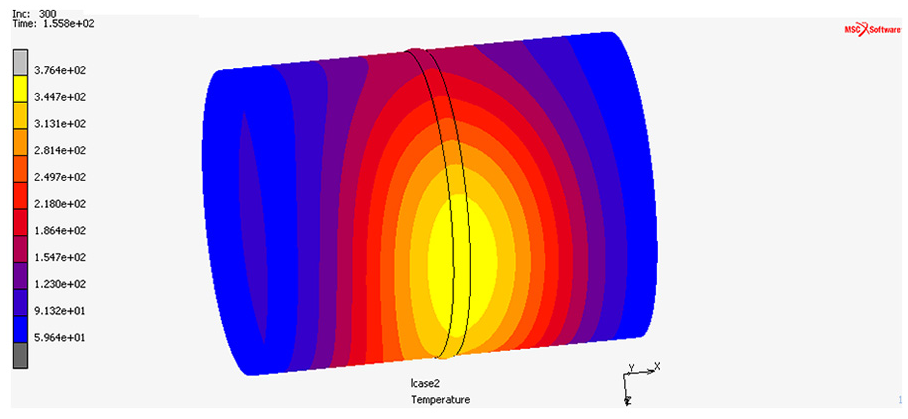
Figure 7(a)–(d) shows the temperature profile at different increments (Inc. 50, 100, 150, and 200) or at different time t = 26.4, 52.8, 79.2, and 105.6 s after the beginning of pipe welding. The temperature profile has been taken when arc at 90° apart on the circumference of the pipe. From Figure 7, it is clear that the temperature of the different nodes varies with the movement of the arc. The thermal profile and the structure of the weld bead are symmetrical with respect to welding axis.

Figure 7.

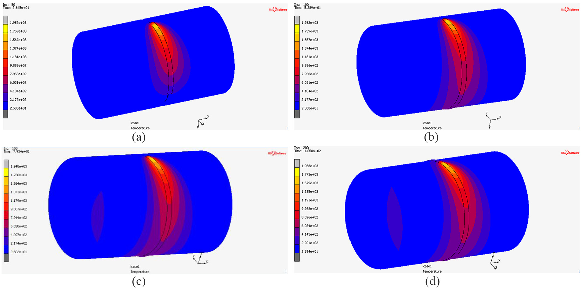
Temperature profile at different time: (a) 26.4 s, (b) 52.8 s, (c) 79.2 s, and (d) 105.6 s.

The maximum temperature is at the weld bead area as anticipated. In front of the heat source, there is a steep temperature gradient, which shows the unimportance of flow of heat in front of the welding arc. To the rear side of the heat source, the cooling phenomenon is shown as the temperature decreases when the arc passes through that certain point. Figure 8 shows the temperature contour after completion of the welding process and after few increment of the time step of the cooling phase.

Figure 8.

The temperature profile after cooling down.

For the axial temperature distribution to different locations on the circumference of the weld pipe, the locations are at 45°, 135°, 225°, and 315°. The steep curve shows that the arc just crosses the section like in the case of Figure 9(a), and the nodes selected for the axial distribution are at 45° from the weld start position in the clockwise direction. 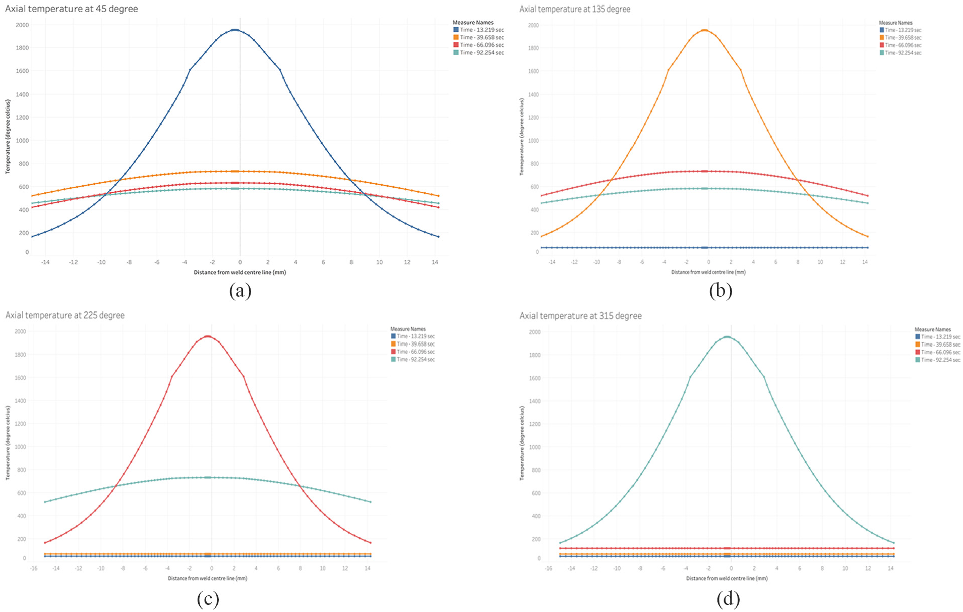The speed of the welding arc is 2.5 mm/s, the total time required to complete welding process is the ration of circumference of the pipe to the speed of the welding arc $(2 \times 3.14 \times 42.11) / 2.5$ that is 105.7 s. To reach at 45°, the time required is 13.22 s, which shows the maximum temperature as anticipated at that particular section. The temperature comes down as the arc moves far from that point. The action of preheating is also shown in the curves as the heat transfer, and the temperature at the other sections is high which is visible in Figure 9. As shown in Figure 9, the section at 225° and 315° is more dominant.

Figure 9.

Axial Temperature Distribution at different locations (a) 45 degree (b) 135 degree (c) 225 degree (d) 315 degree.

The transient thermal cycles at different points of 0, 5, and 10 mm from the weld line and at 90° from the point where the welding process begins are shown in Figure 10. The thermal profile shows the peak value at the time when the arc reaches the corresponding segment, and also apparent from the figure is that the maximum temperature is at 0 mm which is at weld line, while the temperature at the other points which are apart from the weld line has low exponential.

Figure 10.

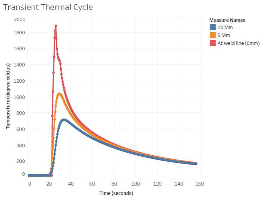
History plot at different points.

Structural analysis

In this analysis, the axial residual stress (the stress which is transverse to the weld bead) which is denoted by the $σ_{x}$ and hoop residual stresses denoted by $σ_{z}$ have been calculated at different sections (45°, 90°, 180°, and 270°) on both the outer and the inner surfaces of the welded pipe. The contour of axial and hoop residual stresses for outer and the inner surfaces of the welded pipe are shown in Figures 11 –14.

Figure 11.

(a) Axial residual stresses contour plot and (b) profile of outer surface of welded pipe.

Figure 12.

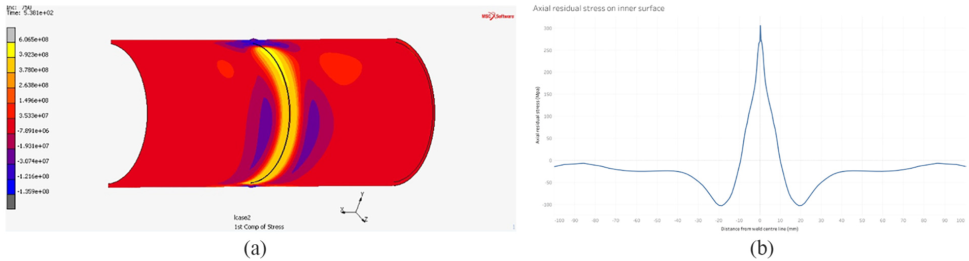
(a) Axial residual stresses contour plot and (b) profile of inner surface of welded pipe.

Figure 13.

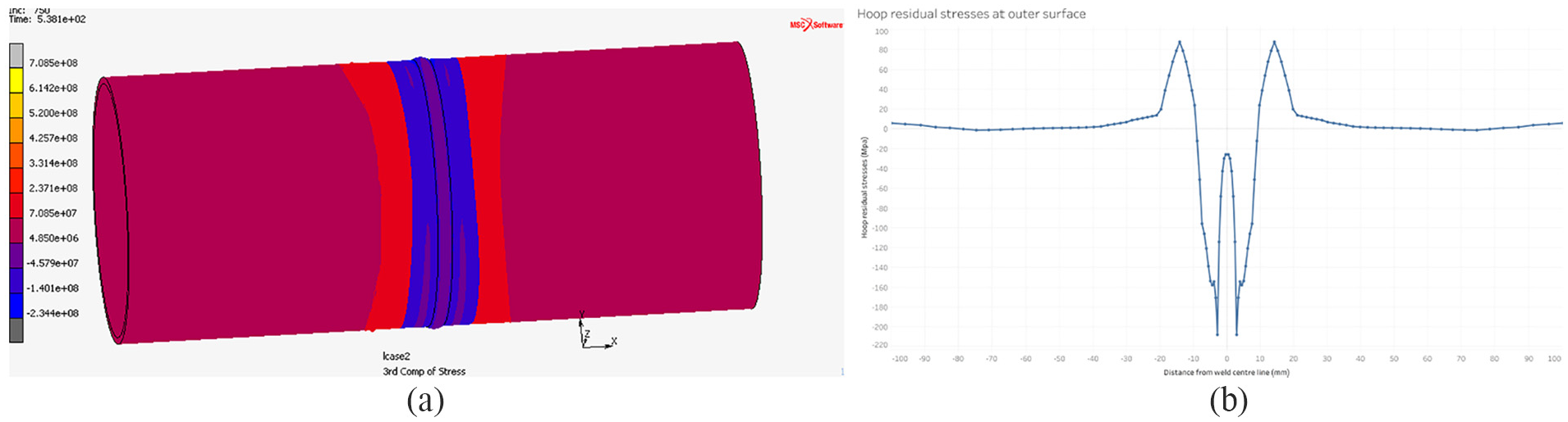
(a) Hoop residual stresses contour plot and (b) outer surface of welded pipe.

Figure 14.

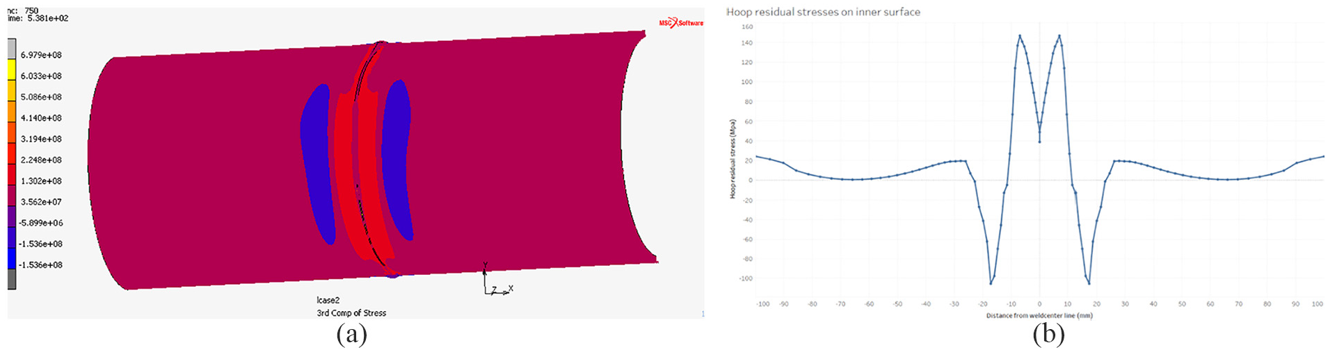
(a) Hoop residual stresses contour plot and (b) inner surface of welded pipe.

Tensile and compressive types of stresses are seen in and around the weld bead area on both the surface area of the welded pipe inner and outer surfaces. This is ascribed to various temperature profiles on both the surfaces of the welded pipe. The variation in the deformation of the thickness of the pipe which is due to the change in the temperature profile across the thickness of the pipe leads to the tensile and compressive stresses in the weld bead on the inner and outer surfaces of the pipe.

There is expansion of the metal when it is heated and contraction happens when the metal gets cool. When the arc passes through the point, the part get heated enough and causes the expansion, and after the arc passes through the point, there is a drastic decrease in the temperature, which is the cooling phase which causes contraction and results in compressive stresses as shown in Figure 15.

Figure 15.

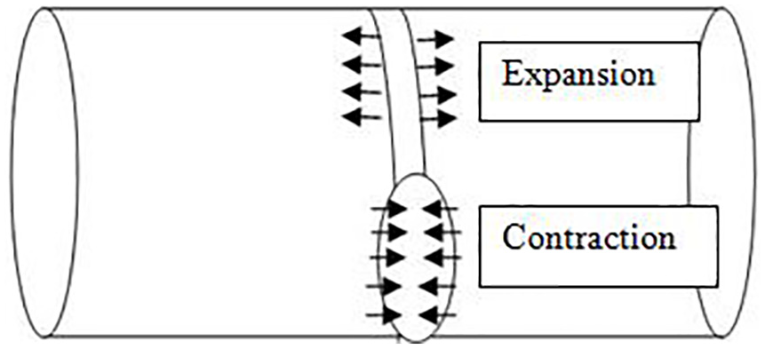
Characteristic of axial residual stresses.

Effect of heat input

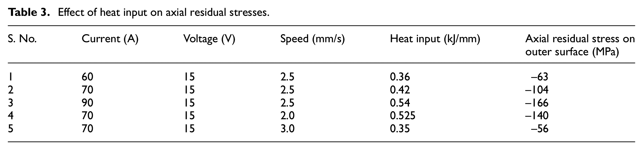
Heat input plays a vital role in controlling the quality of the welding. With the change in the heat input, there is a change in the cooling rate; with the change in the cooling rate, there is effect on the fatigue behaviour of the material, microstructure of the material results in the life of the material. Hence, in this article, the study of the effect of the welding heat input by varying the welding current and the welding speed on the welding residual stresses of the SS-304 is carried out. Five different heat inputs with the change in the current and speed of welding are employed. In Table 3, the longitudinal locked-in stresses on the outer surface at centre of the weld bead of the pipe are given. It can be concluded that with more heat input, there is wider distribution of the compressive longitudinal locked-in stresses in the material. The compressive stresses improve the strength of the material and make the fatigue life of the material longer, which can be achieved by increasing the heat input.

Table 3.

Effect of heat input on axial residual stresses.

S. No.	Current (A)	Voltage (V)	Speed (mm/s)	Heat input (kJ/mm)	Axial residual stress on outer surface (MPa)
1	60	15	2.5	0.36	−63
2	70	15	2.5	0.42	−104
3	90	15	2.5	0.54	−166
4	70	15	2.0	0.525	−140
5	70	15	3.0	0.35	−56

Conclusion

In this study, the FE method was employed to predict the temperature field and the locked-in stresses in the thin cylindrical pipes. According to the outcomes, we concluded the following points:

In view of the distribution of the temperature, near the weld centre and in the HAZ, there is rapid change in the temperature with the distance from the centre point of the welding arc.

In view of the locked-in stresses at the outer surface, there are compressive and the tensile stresses on and around the weld bead and away from the weld bead, respectively.

As we move far away from the weld centre line in the transverse direction, on the outer surface of the welded pipe, the compressive stresses change to the tensile stresses.

The longitudinal residual stresses on the inside surface at different sections have slight change; in this case, the sections near to the weld start have lower values as compared to the other sections.

By increasing the heat input by 35%, there is increase in the axial compressive stresses by 66% at the weld bead, which is due to the high cooling rate.

Footnotes

Acknowledgements

The authors are thankful to Lovely Professional University & IKGPTU, Jalandhar for technical support.

Declaration of conflicting interests

The author(s) declared no potential conflicts of interest with respect to the research, authorship, and/or publication of this article.

Funding

The author(s) received no financial support for the research, authorship, and/or publication of this article.

ORCID iD

Hitesh Arora

References

Kim

. Analysis of welding residual stress formation behavior during circumferential TIG welding of a pipe. Thin Wall Struct 2018; 132: 421–430.

Arora

Singh

Brar

. Thermal and structural modelling of arc welding processes: a literature review. Meas Control 2019; 52: 955–969.

Varma Prasad

Joy Varghese

Suresh

, et al. 3D simulation of residual stress developed during TIG welding of stainless steel pipes. Proc Tech 2016; 24: 364–371.

Malik

Qureshi

Dar

, et al. Residual stress fields under different clamping conditions in circumferentially welded thin-walled cylinders. In: 16th international conference on nuclear engineering, Orlando, FL, 11–15 May 2009, pp. 607–615. New York: ASME.

Qureshi

Malik

Dar

. Residual stress fields due to varying tack welds orientation in circumferentially welded thin-walled cylinders. Adv Mech Eng 2009; 1: 1–9.

Arora

Singh

Hooda

. Studies on temperature variation and angular distortion in submerged arc welded butt joint. Adv Mater Res 2013; 699: 656–661.

Mahapatra

Datta

Pradhan

, et al. Three-dimensional finite element analysis to predict the effects of SAW process parameters on temperature distribution and angular distortions in single-pass butt joints with top and bottom reinforcements. Int J Pres Ves Pip 2006; 83: 721–729.

Hussain

Radi

Majeed

. Study of thermal distortion in thick plate using finite element technique. J Eng Dev 2008; 12: 118–130.

Akbari Mousavi

SAA

Miresmaeili

. Experimental and numerical analyses of residual stress distributions in TIG welding process for 304L stainless steel. J Mater Process Tech 2008; 208: 383–394.

10.

Prakash

Kansal

Pabla

, et al. Effect of surface nano-porosities fabricated by powder mixed electric discharge machining on bone-implant interface: an experimental and finite element study. Nanosci Nanotech Let 2016; 8(10): 1–12.

11.

Malik

Qureshi

Ullah

, et al. Analysis of circumferentially arc welded thin-walled cylinders to investigate the residual stress fields. Thin Wall Struct 2008; 46: 1391–1401.

12.

Bergheau

Fortunier

. Finite element simulation of heat transfer. Hoboken, NJ: Wiley, 2010.

13.

Dhanda

Kanasal

Prakash

. Experimental investigation and optimization of dissimilar joints of AISI 304 and AISI 4140 using pulsed current gas tungsten arc welding process. In: IVth international conference on production and industrial engineering, CPIE-2016, Jalandhar, India, 19–21 December 2016.

14.

Goldak

. Distortion and residual stress in welds: the next generation. In: Proceedings of 8th international conference on trends in welding research, Pine Mountain, GA, 1–6 June 2008.

15.

Hwang

Lee

Kim

, et al. Numerical simulation of welding residual stress distribution on T-joint fillet structure. Int J Ocean Syst Eng 2012; 2: 82–91.

16.

Vemanaboina

Edison

Akella

, et al. Effect of residual stresses of GTA welding for dissimilar materials. Mater Res 2018; 21(4): e20171053.

17.

Hashemzadeh

Chen

Soares

. Evaluation of multi-pass welding-induced residual stress using numerical and experimental approaches. Ships Offshore Struc 2018; 13: 847–856.

18.

Prakash

Bar

Sivaprasad

, et al. The effect of residual stress on fatigue crack growth rate in AISI 304LN stainless steel. Mater Today: Proc 2017; 4: 677–686.

19.

Arya

Singh

Saxena

. Effect of weld cooling rates on mechanical and metallurgical properties of submerged arc welded pressure vessel steel. J Press Vess Technol 2018; 140: 041406.

20.

Chujutalli

Estefen

. Determination of the double-ellipsoid heat source parameters for the numerical simulation of a welding process. In: Proceedings of the 6th international conference on marine structures, Lisbon, 8–10 May 2017.

21.

Chen

Shenoi

. Influence of welding sequence on welding deformation and residual stress of a stiffened plate structure. Ocean Eng 2015; 106: 271–280.

22.

Chen

Hashemzadeh

Garbatov

, et al. Numerical and parametric modeling and analysis of weld-induced residual stresses. Int J Mech Mater Des 2015; 11: 439–453.

23.

Hashemzadeh

Garbatov

Guedes Soares

. Numerical investigation of the thermal fields due to the welding sequences of butt-welds. In: Guedes Soares

Santos

(eds) Maritime technology and engineering. London: CRC Press, 2015, pp. 533–543.

24.

Arora

Singh

Brar

. Finite element simulation of weld-induced residual stress in GTA welded thin cylinders. In: Reference module in materials science and materials engineering. Amsterdam: Elsevier, 2018, pp. 1–13.

25.

Prakash

Singh

Sharma

, et al. Fabrication of aluminium carbon nano tube silicon carbide particles based hybrid nano-composite by spark plasma sintering. Mater Today: Proc 2020; 21: 1637–1642.

26.

Deng

Murakawa

. Numerical simulation of temperature field and residual stress in multi-pass welds in stainless steel pipe and comparison with experimental measurements. Comp Mater Sci 2006; 37: 269–277.

27.

Dar

Qureshi

Hammouda

MMI

. Analysis of weld-induced residual stresses and distortions in thin-walled cylinders. J Mech Sci Technol 2009; 23: 1118–1131.

28.

Deng

Ogawa

Kiyoshima

, et al. Prediction of residual stresses in a dissimilar metal welded pipe with considering cladding, buttering and post weld heat treatment. Comput Mater Sci 2009; 47: 398–408.

29.

Prakash

Singh

. On the characterization of functionally graded biomaterial primed through a novel plaster mold casting process. Mat Sci Eng C 2020; 110: 110654.

30.

Fanous

IFZ

Younan

MYA

Wifi

. 3-D finite element modeling of the welding process using element birth and element movement techniques. J Press Vess Technol 2003; 125: 144–150.

31.

Feli

Aalami Aaleagha

Foroutan

, et al. Finite element simulation of welding sequences effect on residual stresses in multipass butt-welded stainless steel pipes. J Press Vess Technol 2011; 134: 11209.

32.

Perić

Tonković

Rodić

. Numerical analysis and experimental investigation of welding residual stresses and distortions in a T-joint fillet weld. Mater Des 2014; 53: 1052–1063.

33.

Arora

Singh

Brar

. On mechanical and morphological investigations of tungsten inert gas welded SS 304 thin pipe joints. Meas Control 2020; 53: 61–72.

34.

Prakash

Singh

Ramakrishna

, et al. Microwave sintering of porous TieNb-HA composite with high strength and enhanced bioactivity for implant applications. J Alloys Compd 2020; 824: 153774.

35.

Arora

Singh

. Prediction of temperature distribution and displacement of carbon steel plates by FEM. Mater Today: Proc 2019; 18: 3380–3386.

36.

Tiwari

Kumar

, et al. Investigation on micro-residual stress distribution near hole using nanoindentation: effect of drilling speed. Meas Control 2019; 52: 1252–1263.

37.

Nguyen

Chau

Dao

, et al. Experimental study on polishing process of cylindrical roller bearings. Meas Control 2019; 52: 1272–1281.

Numerical simulation on residual stresses of stainless steel SS-304 thin welded pipe

Abstract

Keywords

Introduction

FE simulation

FE model

Thermal analysis

Mechanical analysis

Validation of the model

Experimental procedure

Results and discussion

Thermal analysis

Structural analysis

Effect of heat input

Conclusion

Footnotes

Acknowledgements

Declaration of conflicting interests

Funding

ORCID iD

References