Sage Journals: Discover world-class research

Abstract

Electroencephalogram data are easily affected by artifacts, and a drift may occur during the signal acquisition process. At present, most research focuses on the automatic detection and elimination of artifacts in electrooculograms, electromyograms and electrocardiograms. However, electroencephalogram drift data, which affect the real-time performance, are mainly manually calibrated and abandoned. An emotion classification method based on 1/f fluctuation theory is proposed to classify electroencephalogram data without removing artifacts and drift data. The results show that the proposed method can still achieve a great classification accuracy of 75% in cases in which artifacts and drift data exist when using the support vector machine classifier. In addition, the real-time performance of the proposed method is guaranteed.

Keywords

Emotion classification electroencephalogram 1/f fluctuation K-nearest neighbor support vector machine

Introduction

Electroencephalogram (EEG) signals are time-varying and highly sensitive to various artifacts and interference.^1,2 For example, when the subject slightly moved his or her head, signals of many electrodes significantly undulated during acquisition, that is, the baselines of those electrodes were unstable. These significant undulations are called “drift” in this paper. At present, the main interest of artifacts removing for affective computing is on the eye blink elimination,^3–8 followed by eliminating electrocardiograms (ECGs), electromyograms (EMGs), pulses and other artifacts.^9–12 However, there is hardly any literature dealing with EEG drift data in affective computing, which is determined by how EEG data are analyzed. During the typical processing of offline analysis of event relative potential (ERP), the effect of the lack of partial data is not obvious in the subsequent process, which includes segmenting, superimposing, averaging and so on. Therefore, all the EEG drift data will be rejected in the artificial removal and/or correction stages. Nevertheless, the works of rejecting EEG drift data are usually done manually after acquisition, so that the real-time performance (RTP) of data processing cannot be guaranteed. Moreover, rejecting drift data will interrupt the emotion classification in some special cases. For example, when it is necessary to estimate the emotional state (ES) of the subject continuously or in real time. Li et al.¹³ extracted nine common features from EEG signals without artifacts but with drift, and then proposed a correction method for the EEG drift data in emotion recognition. The results showed that the EEG drift data will cause significant adverse effects on emotion classification.

This study attempts to continuously classify human emotions without rejecting and correcting EEG drift data, which is closer to reality. A method of emotion classification based on 1/f fluctuation theory is proposed. And the RTP of the proposed method is evaluated.

1/f fluctuation theory

A random variation near the macroscopic mean of a physical quantity is called a “fluctuation.” Fluctuations are shown as intuitive phenomena such as the rhythm and intensity of sound changes, and abstract phenomena such as the changes in human emotions and feelings. These fluctuations can be classified according to the corresponding relationship between their power spectral density (PSD) and frequency.

There are three typical fluctuations in nature: 1/f⁰ fluctuations, 1/f² fluctuations and 1/f fluctuations. The 1/f⁰ fluctuation, which has a constant PSD and appears as a straight line parallel to the horizontal axis in the logarithmic coordinate diagram, is often referred to as “white noise.” This fluctuation is completely disordered in the time domain and is irritating. The logarithmic spectrum and time domain waveform of the 1/f⁰ fluctuation are shown in Figure 1.

Figure 1.

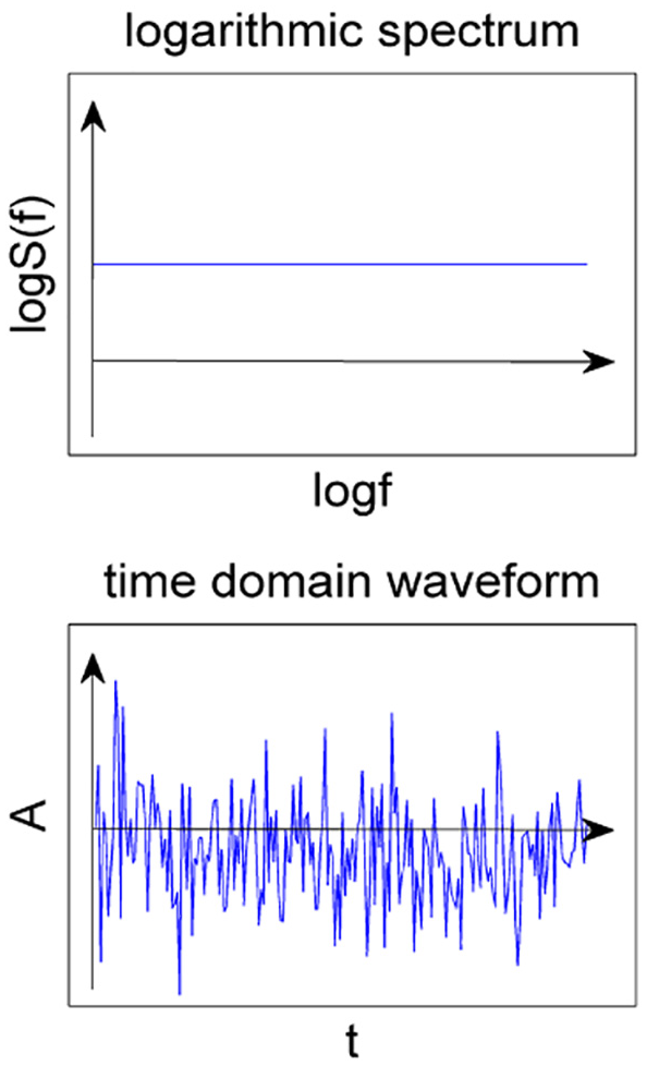
Logarithmic spectrum and time domain waveform of the 1/f⁰ fluctuation.

The 1/f² fluctuation, which has a Lorentz-type power spectrum, is referred as “Brown noise.” This fluctuation has a strong time correlation and is monotonous. The logarithmic spectrum and time domain waveform of the 1/f² fluctuation are shown in Figure 2.

Figure 2.

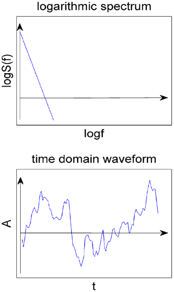
Logarithmic spectrum and time domain waveform of the 1/f² fluctuation.

The randomness and time correlation of the 1/f fluctuation are between those of the 1/f⁰ and 1/f² fluctuations. The logarithmic spectrum and time domain waveform of the 1/f fluctuation are shown in Figure 3.

Figure 3.

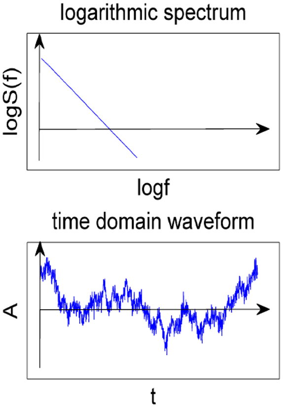
Logarithmic spectrum and time domain waveform of the 1/f fluctuation.

The 1/f fluctuation is generally comfortable. In the 1970s, the Japanese physicist Toshimitu¹⁴ gave an explanation from the perspective of chaos theory. He proposed that the 1/f fluctuation can make people feel comfortable because the fluctuations of the heartbeat cycle and the α rhythm (8–13 Hz) of the EEG in a quiet state are in good agreement with the 1/f fluctuation. In addition, he also believed that external stimuli that are consistent with the 1/f fluctuation will make people feel comfortable.

Materials

Models of emotions

Scholars believe that all human emotions can be derived from the basic emotion set, and they have put forward different basic emotion sets. For example, James’s basic emotion set included anger, fear, sadness and love, while Ekman’s set included anger, fear, sadness, happiness, disgust and surprise.¹⁵ Studies found that there are certain correlations between some emotions. For example, anger and disgust sometimes occur simultaneously. Therefore, some scholars described emotions in different dimensions according to these correlations. Davidson et al.¹⁶ and Lang et al.¹⁷ presented their own two-dimensional (2D) emotional models. In addition, some researchers have described a three-dimensional (3D) emotional model, in which the three dimensions are pleasure, arousal and dominance (PAD).^18,19 This study used Lang’s emotional model, which is shown in Figure 4, to evaluate stimuli materials. The abscissa indicates the valence, and the ordinate indicates the arousal in the Lang’s model.

Figure 4.

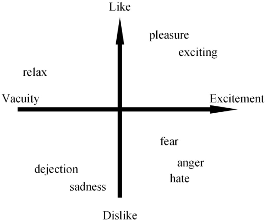
Lang et al.’s¹⁷ 2D emotional model.

Music stimuli

The external stimuli induction method was used to induce different emotions in the subjects in the experiments. To effectively induce the ES of the subjects, it is necessary to objectively evaluate the stimuli materials. Therefore, all the audio files were downloaded from the Internet and evaluated via Lang’s model. Then, six audio clips ranging from 30 to 45 s were chosen as stimuli, half of which were positive and the other half were negative. All audio clips are in wav format and dual tracks with a sampling rate of 44.1 kHz.

Statement of ethics and human rights

All subjects signed informed consent forms before the experiments, which was approved by the Beihang University ethical review committee (IRB). All procedures that were performed in studies involving human participants were in accordance with the ethical standards of the institutional and/or national research committee and with the 1964 Helsinki declaration and its later amendments or comparable ethical standards.

Participants

A total of 12 volunteers participated in this study. They were divided into two groups: the evaluation group and the acquisition group. Each volunteer joined only one group. The evaluation group consisted of three males and three females, and did not participant in EEG data acquisition. The acquisition group consisted of six males, and all the EEG data used in this study were from them.

All participants were healthy, right-handed postgraduate students. The age ranged from 22 to 26 years in the evaluation group and from 22 to 36 years in the acquisition group. All participants had no personal history of neurological or psychiatric illnesses, and did not receive professional music training. The emotional evocation and EEG data acquisition were completed in a closed and quiet room to reduce the interference.

EEG data

EEG data were recorded with a 64-channel electrical signal imaging system (Neuro Scan Labs), the SCAN 4.5 software and a 64-channel Quick Cap with embedded Ag/AgCl electrodes. Those electrodes were arranged according to the extended international 10–20 system. The impedance was kept below 5 kΩ. The EEG data were recorded at the sampling rate of 1000 Hz. Experimental scenario and device are shown in Figure 5. Part (a) shows the corresponding resistance of each electrode when injecting the conductive gel. Part (b) shows the EEG amplifier used in the experiment.

Figure 5.

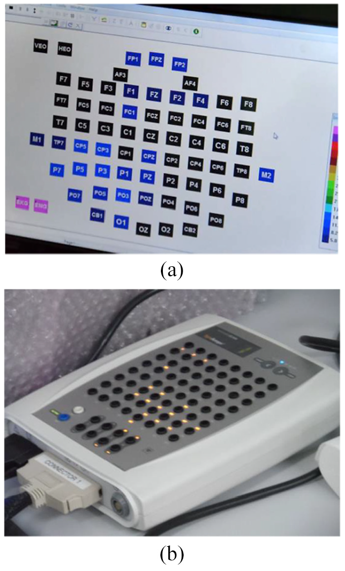
Some experimental devices and scenarios: (a) resistance of each electrode and (b) EEG amplifier.

Two desktops were used during the acquisition of EEG signals. One of them played music stimuli, and the other stored corresponding EEG data. The music stimuli were played in the order that all positive stimuli were played first, followed by all negative stimuli. The time interval between playing two adjacent stimuli was more than 60 s, so that the participants could return to the calm state. And each music stimulus was played after the participants indicated that they were ready. Research showed that the most influential human electrical signal to EEG is electrooculogram (EOG).²⁰ However, using music stimuli to induce EEG signals does not require the use of vision. Therefore, all the participants were required to keep their eyes closed during EEG data acquisition to minimize EOG artifacts.

Methods

Pleasant external stimuli will stimulate brain waves with a fluctuation feature (FF) of about –45° according to the 1/f fluctuation theory. Therefore, the FFs of the EEGs that are stimulated by positive music stimuli should be closer to –45° than those stimulated by negative music stimuli. The ES of EEGs can be determined by comparing the difference between the FFs of EEGs and those of different music stimuli.

Two groups of experiments were carried out in this study, and the corresponding flowcharts are shown in Figure 6. In both groups of experiments, the features of the music stimuli were directly extracted, and the EEG data were preprocessed before the feature extraction. Then, all the features were directly input into the classification in group A, while channel selection was carried out before classification in group B.

Figure 6.

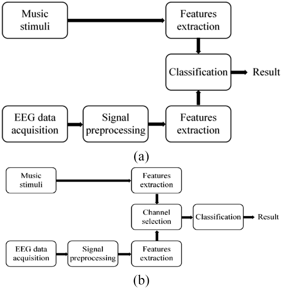
The flowcharts of two groups of experiments in this study—(a) group A: classification without channel selection and (b) group B: classification with channel selection.

EEG data preprocessing

The only preprocessing was filtering. A low-pass filter with a cut-off frequency of 50 Hz was used to filter the time domain waveform of the EEG data. There are three reasons for this. One reason is to minimize the processing delay to ensure the RTP. Another is that since the most influence (i.e. EOG) could be ignored, other artifacts could also be ignored. The last is to measure the classification performance under the condition of a minimal signal-to-noise rate.

Feature extraction

The extraction procedures of FFs of music stimuli and EEG data were basically the same, but there were differences according to the signal characteristics. The reason for using angles instead of slope values is that the changes of angles are more linear than the changes of slope values.

Music stimuli

The steps of the feature extraction of music stimuli are as follows:

The time domain waveforms of the data were segmented into segments with the same length.

The fast Fourier transform (FFT) was used to calculate the PSD of each segment.

The PSD below 20 kHz was intercepted and converted to the logarithmic spectrum.

Linear fitting was carried out for the logarithmic spectrum.

The slope of the fitting line was converted to an angle using the inverse trigonometric function. These angles were regarded as the FFs.

EEG data

The steps of feature extraction for EEG data were almost the same as those for music stimuli, but with a few differences. One was that the objects of the segmentation and FFT were EEG data. Another was that the frequency interception range in the third step was 0.5–45 Hz. The obtained angles were regarded as the FFs of EEG data.

Channel selection

Studies showed that there is a correlation between different regions of the brain and different emotions.^21–24 Therefore, the accuracy of the emotion classification will be improved using the proper electrode. And electrode is also referred to as “channel” for ease of understanding in the following. The differences of the FFs between the channels and the music stimuli were calculated. And then a few channels with smaller total difference values were selected for the emotion classification, as shown in expression (1)

CH_S_{i} \propto min (Δ θ_{j, k}) = min (| θ_{channe l_{j}} - θ_{stimul i_{k}} |)

(1)

where $θ_{channe l_{j}}$ is the FF of the $j th$ channel, $θ_{stimul i_{k}}$ is the FF of the $k th$ music stimuli, $Δ θ_{j, k}$ is the difference between them and $CH_S_{i}$ is the $i th$ channel selected.

Emotion classification

Classification without channel selection

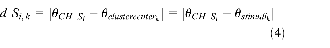
K-nearest neighbor (KNN) and support vector machine (SVM) classifiers were used for the emotion classification. The FFs of EEG data expressing positive emotions should be closer to –45° than those of EEG data expressing negative emotions according to the 1/f fluctuation theory. Therefore, the FFs of all music stimuli were used as the cluster centers in the KNN classifier. The Euclidean distance between the FF from a channel and a cluster center was calculated as follows

d_{i, k} = | θ_{C H_{i}} - θ_{clustercente r_{k}} | = | θ_{C H_{i}} - θ_{stimul i_{k}} |

(2)

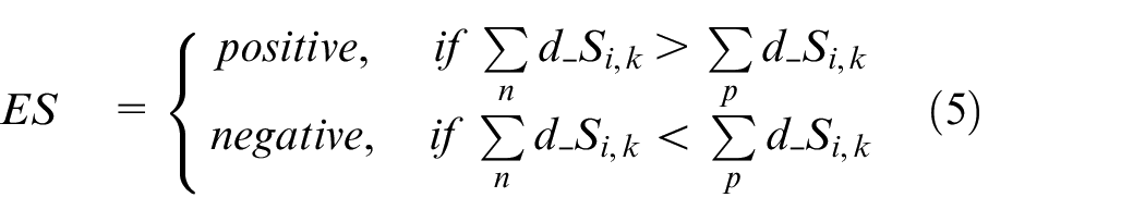
Then, the current ES of that channel was determined with a smaller sum of distances, which is shown as follows

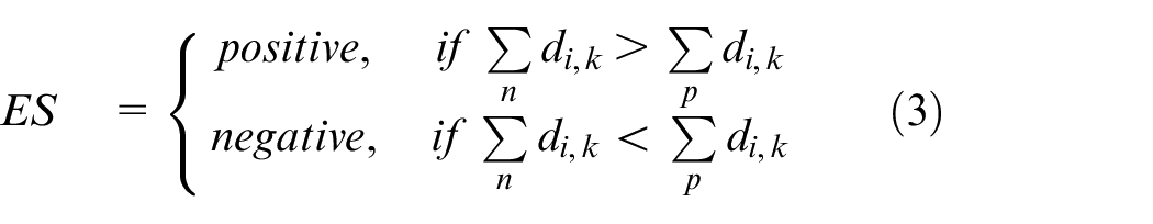
\begin{matrix} ES & = {\begin{matrix} positive, & if \sum_{n} d_{i, k} > \sum_{p} d_{i, k} \\ negative, & if \sum_{n} d_{i, k} < \sum_{p} d_{i, k} \end{matrix} \end{matrix}

(3)

where $\sum_{n} d_{i, k}$ is the sum of the Euclidean distances between channels and negative cluster centers, while $\sum_{p} d_{i, k}$ is the sum of the distances between channels and positive ones.

Classification with channel selection

KNN and SVM classifiers were used for emotion classification. As shown in expression (4), the FFs of all music stimuli were used as the cluster centers in the KNN classifier. The Euclidean distance between the FF from a selected channel and a cluster center was calculated as follows

d_S_{i, k} = | θ_{CH_S_{i}} - θ_{clustercente r_{k}} | = | θ_{CH_S_{i}} - θ_{stimul i_{k}} |

(4)

Then, the current ES of that channel was determined with a smaller sum of distances, which is shown as follows

\begin{matrix} ES & = {\begin{matrix} positive, & if \sum_{n} d_S_{i, k} > \sum_{p} d_S_{i, k} \\ negative, & if \sum_{n} d_S_{i, k} < \sum_{p} d_S_{i, k} \end{matrix} \end{matrix}

(5)

Experimental results

The authors calculated the FFs of the music stimuli. According to the 1/f fluctuation theory, these angles of different external stimuli should be different, and the pleasant external stimuli should have an FF of about –45°. Then, the authors compared the proposed method with the comparison method using the classification accuracy and the average time consumption (TC) of each segment of EEG data (500 ms) as the performance indicators. The leave-one-out method was used when using the SVM classifier because the classification accuracies of the 10-fold method were generally lower. The average TC was also calculated based on the total TC of multiple operations on all data.

Empirical mode decomposition (EMD) is a time-frequency analysis method for adaptive signals, which has obvious advantages in processing non-stationary nonlinear random signals such as EEG signals. A number of intrinsic mode function (IMF) sequences arranged from high to low frequencies with different frequency ranges will be obtained after EMD. EMD/IMF was used in emotion recognition in recent years.^25–27 And some nonlinear features, such as approximate entropy (AE), energy entropy (EE) and energy moment (EM), were used in existing works.^27–29 Therefore, the features and the methods mentioned above were compared with the proposed method.

Evaluation and 1/f FFs of music stimuli

The evaluation criteria for music stimuli were as follows: like ∼9 to dislike ∼1; and excitement ∼9 to vacuity ∼1. The mean values of the evaluation are shown in Table 1. The evaluation criteria were explained before the participants listened to the music clips, but the emotion that was expressed in every clip was not given in advance. Table 1 illustrates that the positive music stimuli have better emotion discrimination and excitation effects according to the 1/f fluctuation theory.

Table 1.

Evaluation and average FF of stimuli.

Stimuli number	Emotion type	Valence	Arousal	Average FF
1	Positive	7.5	7	–44.00°
2	Positive	7	7.67	–45.06°
3	Positive	7.33	7.17	–44.93°
4	Negative	3.17	6.67	–52.98°
5	Negative	2.33	7.67	–51.93°
6	Negative	2.83	7.17	–52.75°

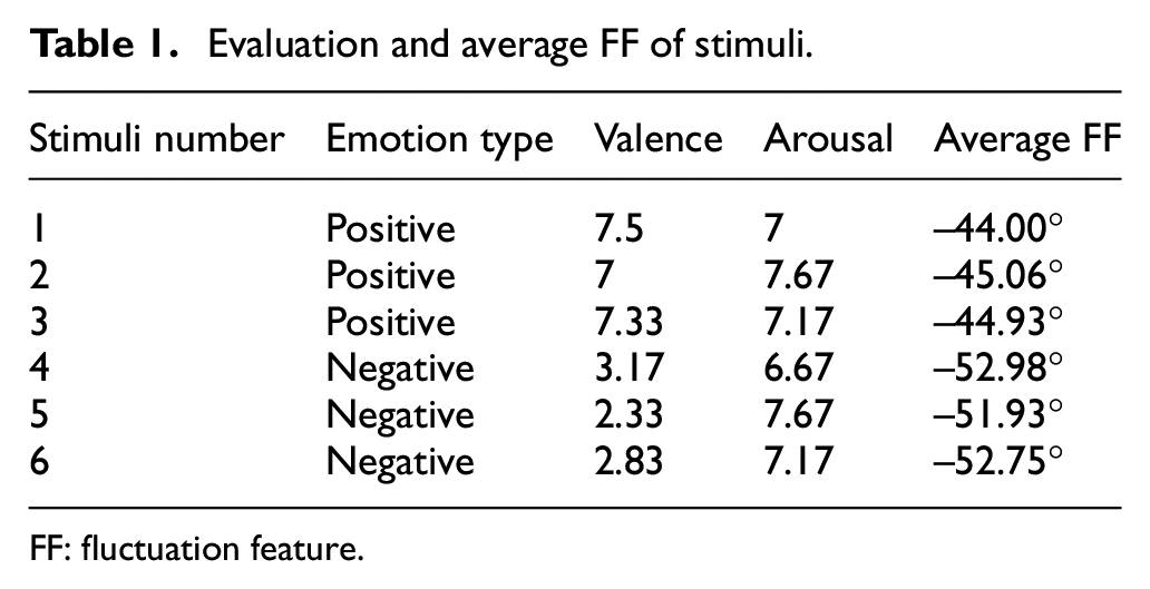
FF: fluctuation feature.

However, the 1/f fluctuation theory does not directly indicate the FFs of negative emotions. The negative music stimuli that were used in this study were sad music. The authors believed that their FFs should be closer to those of the 1/f² fluctuation. Therefore, the rationality of the FFs of negative music stimuli should be verified. Some of Bach’s music, which was said to be sorrowful and heavy, were downloaded from the Internet. Then, their average FFs and evaluations are shown in Table 2. It was known that the negative stimuli were appropriate for stimulating negative emotions by comparing the average FF and evaluation of Bach’s music with those of the negative music stimuli. Therefore, these six average FFs in Table 1 were used as the cluster centers in KNN classifier.

Table 2.

Evaluation and average FF of some Bach’s music.

Music name	Valence	Arousal	Average FF
Air for the G string	2.83	4.83	–49.42°
Air on the G string	2.67	4.83	–50.35°
Air-Suite No. 3 In D Major	3	5.33	–49.14°
Arioso For Brass	5.17	5	–49.73°
Cello Suite No. 1 in G major	3.33	6	–48.77°
Jesu, Joy Of Mans Desiring	5	5.17	–49.84°

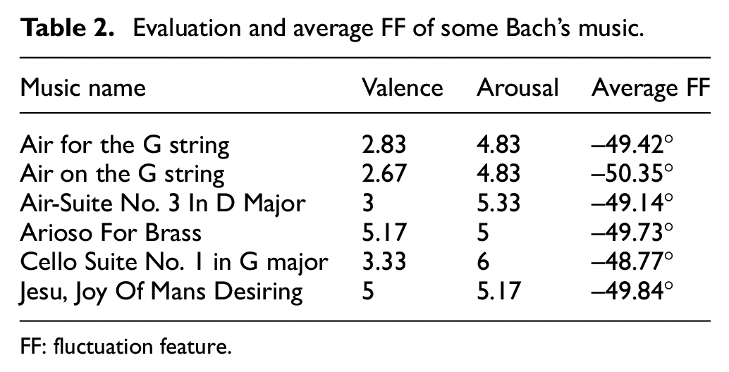
FF: fluctuation feature.

Emotion classification without channel selection

There are 3366 EEG data segments in all, of which 2278 segments are from positive excitations and 1088 segments are from negative excitations. All features were directly classified by the KNN classifier with the average FFs of the music stimuli as the clustering centers, that is, experiment A1. The results showed that the average accuracy rate of the classification is 65.48%. All features were directly classified by the SVM classifier in experiment A2, and the recognition accuracy reached 75%.

EEG channel selection

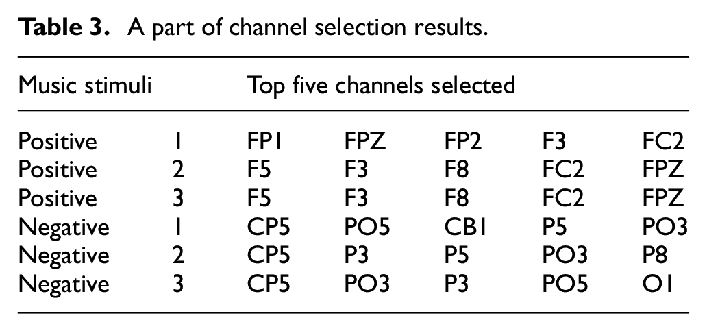
Three groups of experiments were carried out, which were called B1, B2 and B3. In experiment B1, the differences of the FFs between channels and music stimuli were calculated and screened. The selection results were different in similar music, as shown in Table 3. After comparing the sorted results, F5, F3, FC2, F8, FPZ and FP2 were selected as positive optional channels for emotion classification, while CP5, P5P3, PO5, PO3 and O1 were selected as negative ones. In experiment B2, a positive channel and a negative channel were arranged into a group of one-by-one channel pairs for classification. In experiment B3, two positive channels and two negative channels were arranged into a group of two-by-two channel pairs for classification. And the classification results of B1, B2 and B3 will be described in section “Emotion classification with channel selection.”

Table 3.

A part of channel selection results.

Music stimuli		Top five channels selected
Positive	1	FP1	FPZ	FP2	F3	FC2
Positive	2	F5	F3	F8	FC2	FPZ
Positive	3	F5	F3	F8	FC2	FPZ
Negative	1	CP5	PO5	CB1	P5	PO3
Negative	2	CP5	P3	P5	PO3	P8
Negative	3	CP5	PO3	P3	PO5	O1

Emotion classification with channel selection

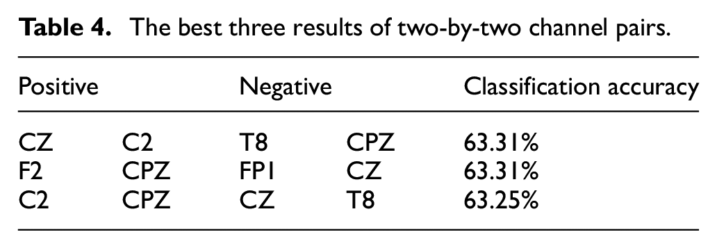
The best three results of the classification accuracy of the channels selected in experiment B1 were 58.23% (FC2-O1), 57.96% (FC2-PO3) and 57.81% (FC2-CP5), respectively. The best three results of the one-by-one channel pairs were 62.36% (CPZ-CZ), 62.33% (CZ-FC2) and 62.33% (CZ-C2), respectively. Table 4 gives the three best results of the two-by-two channel pairs. The above results showed that the classification accuracy increased with the number of channels participating in the classification. However, the simulation also showed that channel selection does not improve the classification performance, which is inconsistent with the results of related studies.^30,31 The authors believed that classifications with only parts of channels will lead to insufficient effective information and decrease the classification accuracy in the case of EEG data containing artifacts and interference. Unlike the data that were used in this work, artifacts and interference were removed from the data that were used in related studies. Therefore, channel selection was conductive to eliminating the impact of non-task EEG components and improving the classification performance in those studies.

Table 4.

The best three results of two-by-two channel pairs.

Positive		Negative		Classification accuracy
CZ	C2	T8	CPZ	63.31%
F2	CPZ	FP1	CZ	63.31%
C2	CPZ	CZ	T8	63.25%

Moreover, the three-by-three channel pairs were not tested because approximately 1.5*10⁹ sets of data need to be calculated for 70 continuous days. This is beyond the computing power of the computer that was used by the authors.

RTP

The RTP of the feature extraction and classification was analyzed. The main parameters of the computer are as follows: an i7 3.4 GHz CPU, and 8 GB of RAM. The corresponding EEG signals are called a group of data when a participant listened to a music stimulus. A group of data were loaded into MATLAB and then divided into segments with durations of 500 ms in the simulation. The last part of the data that was less than 500 ms was complemented by “0”s. The average TC of each segment varied with the amount of data in the feature extraction phase. For example, if 60 segments were input into the calculation at one time, the average extraction TC was approximately 20 ms, while it was approximately 110 ms if 600 segments were input into the calculation at one time. The results showed that the increasing rate of the extraction TC is smaller than that of the amount of data. The reason is that MATLAB is sensitive to the amount of data in the calculation process, which results in the change of the unit processing time of data with those amounts. Figure 7 illustrates the relationship between the amount of data and the TC per segment in the simulation. The measured curve is almost a straight line, which means that the average TC will be approximately 10 ms if only a few segments are put into calculation.

Figure 7.

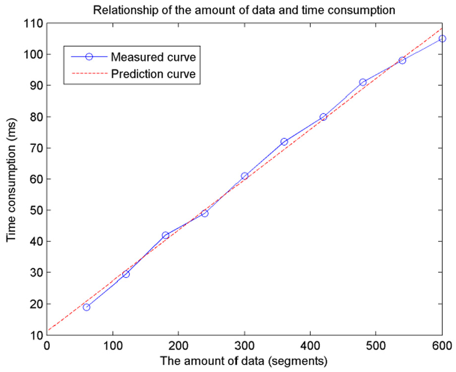
Relationship between the amount of data and time consumption.

The average extraction TC of the AE was approximately 30 ms, and it hardly varied with the amount of the data. This means that the RTP cannot be improved even with small amounts of data. The average extraction TC of the IMF was related to the number of IMF components and was less related to the amount of EEG data. The total average extraction TC of the IMF was approximately 75 ms according to the simulation. Since the TC for calculating EE and EM was too short, it was negligible compared with the TC for extracting IMF.

The average TC of each segment was less than 0.1 ms when the KNN classifier was used. This means that the TC of the classification itself is essentially negligible regardless of whether the channel selection has been carried out. The average TC of each data segment was approximately 250 ms in the SVM classification, which includes the training time of the classification model. However, if only the label prediction was considered, the average TC for each segment was approximately 0.2 ms.

Comparison

Table 5 compares the classification performance of the proposed method with those of several existing methods. All methods used music stimuli to stimulate emotional EEG. And all methods were compared in terms of features, classifiers, accuracies and average TC. The results illustrate that the proposed method can balance the accuracy and RTP of emotion recognition. The simulations showed that the average TC of the proposed method is the smaller when the classification accuracy is similar while the accuracy is high when the TC is similar. All the results were obtained without removing the drift and interference in the EEG data. The average TC was obtained by processing data segments with duration of 500 ms from feature extraction to classification when all available data were put into the calculation at one time.

Table 5.

Comparison of the classification results.

Method	Feature	Classifier	Accuracy (%)	Average TC(ms)
				Feature extraction	Classification
Proposed method	Angle of 1/f	KNN	65.48	Approximate linear variation with data quantity	0.1
		SVM	75		250
Lu et al.²⁷	AE	KNN	59.38	30	0.1
	EE of IMF	KNN	65.83	75	0.1
	EM of IMF	KNN	56.15	75	0.1
Wang et al.²⁸	AE	SVM	77.63	30	250
	EE of IMF	SVM	72.04	75	250
	EM of IMF	SVM	67.58	75	250

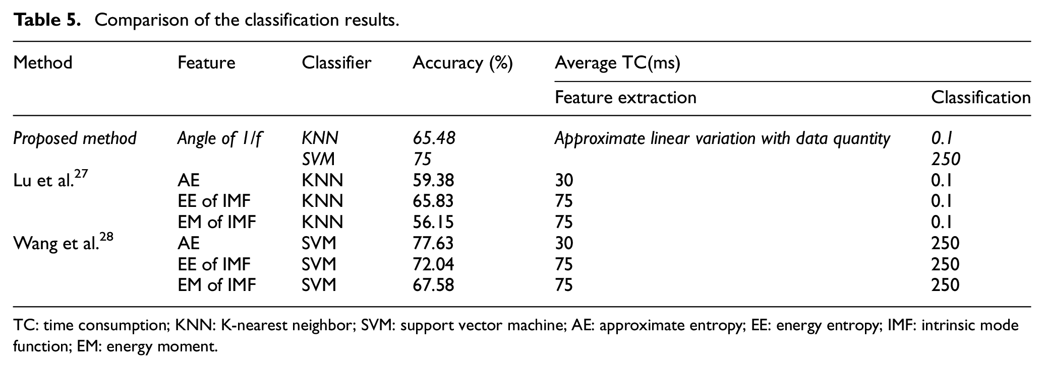
TC: time consumption; KNN: K-nearest neighbor; SVM: support vector machine; AE: approximate entropy; EE: energy entropy; IMF: intrinsic mode function; EM: energy moment.

Conclusion

For emotional recognition applications with high real-time requirements, the most important goal is not to obtain a higher classification accuracy, but rather a higher processing speed and a smaller processing delay. This study used EEG data that were only low-pass filtered to maximize real-time processing. The proposed method achieves a great classification accuracy of 75% in cases in which artifacts and drift data exist. In addition, the TC of the feature extraction and classification is low. If the classification accuracy can be improved while maintaining the RTP, the results of this study will have good applicability, such as for monitoring the ES changes of astronauts, vehicle drivers and crew and even ordinary soldiers in the operations. The future development of this research will attempt to increase the artifact removal procedure under the premise of ensuring a RTP and extract more effective features to improve the accuracy of emotion recognition.

Footnotes

Declaration of conflicting interests

The author(s) declared no potential conflicts of interest with respect to the research, authorship and/or publication of this article.

Funding

The author(s) disclosed receipt of the following financial support for the research, authorship and/or publication of this article: This work was supported in part by Specialized Research Fund for the Doctoral Program of Higher Education (SRFDP) under grant 20121102130001, the National Science Foundation for Young Scientists of China under grant 61603013 and the Fundamental Research Funds for the Central Universities (No. YWF-19-BJ-Y-197).

ORCID iD

Lijiang Chen

References

Zhao

Experimental tutorials of ERPs. Revised ed. Nanjing, China: Southeast University Press, 2010.

Zhu

, et al. Removal of artifacts from EEG signal. J Biomed Eng 2008; 25(2): 464–471.

Gomez-Herrero

De Clercq

Anwar

, et al. Automatic removal of ocular artifacts in the EEG without an EOG reference channel. In: Proceedings of the 7th Nordic signal processing symposium, Reykjavik, 7–9 June 2006, pp. 130–133. New York: IEEE.

Benkherrat

Bouguerra

Choufa

Removal of ocular artifacts from related evoked potentials using VSSLMS adaptive filter. In: Proceedings of the international conference on “computer as a tool,”Warsaw, 9–12 September 2007, pp. 349–352. New York: IEEE.

Zhu

Tong

Chen

YQ.

An ICA-based method for automatic eye blink artifact correction in multi-channel EEG. In: Proceedings of the 5th international conference on information technology and applications in biomedicine, Shenzhen, China, 30–31 May 2008, pp. 338–341. New York: IEEE.

Shen

Shi

JH.

Automatic ocular artifact removal based on blind source separation. J Zhejiang Univ (Eng Sci) 2013; 47(3): 415–421, 464.

Peng

Shi

, et al. Removal of ocular artifacts in EEG–an improved approach combining DWT and ANC for portable applications. IEEE J Biomed Health Inform 2013; 17(3): 600–607.

Mahajan

Morshed

BI.

Unsupervised eye blink artifact denoising of EEG data with modified multiscale sample entropy, kurtosis, and wavelet-ICA. IEEE J Biomed Health Inform 2015; 19(1): 158–165.

Shao

Shen

Ong

, et al. Automatic EEG artifact removal: a weighted support vector machine approach with error correction. IEEE Trans Biomed Eng 2009; 56(2): 336–344.

10.

Wang

Lin

Zhang

, et al. EMD-based EEG signal enhancement for auditory evoked potential recovery under high stimulus-rate paradigm. Biomed Signal Process Control 2013; 8: 858–868.

11.

Ferdowsi

Sanei

Abolghasemi

, et al. Removing ballistocardiogram artifact from EEG using short- and long-term linear predictor. IEEE Trans Biomed Eng 2013; 60(7): 1900–1911.

12.

Hamaneh

Chitravas

Kaiboriboon

, et al. Automated removal of EKG artifact from EEG data using independent component analysis and continuous wavelet transformation. IEEE Trans Biomed Eng 2014; 61(6): 1634–1641.

13.

Mao

Liang

XG.

Correction method of EEG drift data in emotion recognition. J Huazhong Univ Sci Technol 2017; 45(9): 28–32.

14.

Toshimitu

Reflections on fluctuation: the mystery of 1/f fluctuation. Tokyo, Japan: NHK Press, 1994.

15.

Healey

Wearable and automotive systems for affect recognition from physiology. Doctoral Thesis, MIT, Cambridge, MA, 2000, https://www.researchgate.net/publication/34526399_Wearable_and_automotive_systems_for_affect_recognition_from_physiology

16.

Davidson

Schwartz

Saron

, et al. Frontal versus parietal EEG asymmetry during positive and negative affect. Psychophysiology 1979; 16: 202–203.

17.

Lang

Bradley

Cuthbert

, et al. International affective picture system (IAPS): technical manual and affective ratings. Gainesville, FL: University of Florida, 1999.

18.

Ekman

Davidson

The nature of emotion: fundamental questions. Oxford: Oxford University Press, 1994.

19.

Mehrabian

Pleasure-arousal-dominance: a general framework for describing and measuring individual differences in temperament. Curr Psychol 1996; 14(4): 261–292.

20.

Wei

CQ.

Concise tutorial on medical electronics. Beijing, China: Medical University Press, 1994.

21.

Nie

Wang

Shi

, et al. EEG-based emotion recognition during watching movies. In: Proceedings of the 5th international IEEE/EMBS conference on neural engineering, Cancun, Mexico, 27 April–1 May 2011, pp. 667–670. New York: IEEE.

22.

Schmidt

Trainor

LJ.

Frontal brain electrical activity (EEG) distinguishes valence and intensity of musical emotions. Cognit Emot 2001; 15(4): 487–500.

23.

Sarlo

Buodo

Poli

, et al. Changes in EEG alpha power to different disgust elicitors: the specificity of mutilations. Neurosci Lett 2005; 382: 291–296.

24.

Petrantonakis

Hadjileontiadis

LJ.

A novel emotion elicitation index using frontal brain asymmetry for enhanced EEG-based emotion recognition. IEEE Trans Inform Technol Biomed 2011; 15(5): 737–746.

25.

Yang

Chen

DW.

Application of Hilbert-Huang transform in emotion EEG feature extraction. Comput Eng Des 2014; 35(7): 2509–2514.

26.

Mert

Akan

Emotion recognition from EEG signals by using multivariate empirical mode decomposition. Pattern Anal Appl 2018; 21(1): 81–89.

27.

Zou

Zhang

, et al. Emotion electroencephalograph (EEG) recognition based on IMF energy entropy. J Biomed Eng Res 2016; 32(2): 71–74.

28.

Wang

Wei

TY.

Research on EEG emotion feature extraction based on IMF energy moment. Modern Electron Tech 2018; 41(20): 10–13.

29.

Cao

Xiang

Comparative study of approximate entropy and sample entropy based on characterization of EEG. Comput Eng Des 2014; 35(3): 1021–1026.

30.

Ansari-Asl

Chanel

Pun

A channel selection method for EEG classification in emotion assessment based on synchronization likelihood. In: Proceedings of the 15th European signal processing conference (EUSIPCO 2007), Poznan, 2007, pp. 1241–1245, https://www.eurasip.org/Proceedings/Eusipco/Eusipco2007/Papers/c1l-e03.pdf

31.

Wang

Nie

BL.

EEG-based emotion recognition using frequency domain features and support vector machines. In: Proceedings of the international conference on neural information processing (ICONIP 2011), Berlin, 2011, pp. 734–743, https://www.researchgate.net/publication/221139865_EEG-Based_Emotion_Recognition_Using_Frequency_Domain_Features_and_Support_Vector_Machines

An emotion classification method from electroencephalogram based on 1/f fluctuation theory

Abstract

Keywords

Introduction

1/f fluctuation theory

Materials

Models of emotions

Music stimuli

Statement of ethics and human rights

Participants

EEG data

Methods

EEG data preprocessing

Feature extraction

Music stimuli

EEG data

Channel selection

Emotion classification

Classification without channel selection

Classification with channel selection

Experimental results

Evaluation and 1/f FFs of music stimuli

Emotion classification without channel selection

EEG channel selection

Emotion classification with channel selection

RTP

Comparison

Conclusion

Footnotes

Declaration of conflicting interests

Funding

ORCID iD

References