
Abstract
In the original model reference adaptive induction motor speed sensorless system based on flux linkage, there is a large fluctuation of the rotational speed in transient and steady state. When the motor speed is estimated, the integral part of voltage model affects the accuracy of the estimated speed with high-frequency signals and noise. In order to solve the above problems and further improve the system’s anti-interference performance and the speed estimation accuracy at low speed, an improved method of speed estimation that combines fuzzy proportional integral control and sliding mode control is proposed, by adopting genetic algorithm to optimize the parameters of the three sliding mode controllers, meanwhile, using the error integration criterion as the objective function of genetic algorithm optimization and searching for the optimal value of the objective function. Compared to the conventional method, the simulation results show the effectiveness of the proposed method in the middle- and low-speed regions with improved robustness against external disturbance, also display the high accuracy of estimated speed, the minor amplitude and frequency of speed fluctuation, and the great dynamic performance indexes of the system.
Introduction
Since the 20th century, with the increasing demand for electric power transmission, AC motor drive based on induction motor has attracted great attention. It is proposed that induction motor is a multivariable, nonlinear, and strong coupling object. In order to obtain high dynamic speed regulation performance, it is necessary to study the speed regulation scheme of high performance induction motor from dynamic model. 1 In 1972, Blaschke proposed the theory of magnetic field orientation, which controlled the induction motor as the DC motor, making the vector-controlled AC variable-voltage variable-frequency speed control system comparable to the DC-speed control system in terms of static and dynamic performance. 2 In order to obtain good speed control performance, the traditional induction motor vector control system detects the motor speed through a photoelectric encoder, a speed encoder is undesirable in a drive. It not only adds costs but also there is a problem about concentricity in the installation on the motor shaft. 3 The proposed sensorless vector control solves these problems aptly. The sensorless vector control is used to estimate the motor speed through the observer. So far, motor speed estimation methods are mainly divided into back electromotive force (EMF) model method and signal injection method. The back EMF model methods mainly include model referencing adaptive system and extended Kalman filter. Extended Kalman filter is to make the linear system estimation algorithm apply to nonlinear systems, which deals with a series of problems caused by parameters variation and noise pollution effectively. However, this computationally intensive method is time consuming, and there are also many parameters needed to be adjusted. Provided the parameters setting is unsuitable, it affects the convergence speed, and even causes system instability as well as increase the difficulty of practical application.4–6 Signal injection methods mainly include high-frequency signal injection method, rotor tooth harmonic method, and so on. 7 It is to inject a specific voltage (current) signal into the stator or rotor side of the motor, and then detects a corresponding current (voltage) signal in the motor to determine the salient pole position of the rotor. This method is immune from changes of motor parameters. However, the injected signal affects the normal operation of the motor and the accuracy of the speed estimation. 8 Compared with above methods, the structure of model reference adaptive system (MRAS) used in this paper is simple, whose estimated speed is easy to converge and has high precision. After many years of theoretical development of MRAS, domestic and foreign scholars have developed a variety of speed estimation methods based on different reference models and adjustable models. There are three common MRAS models: (1) voltage model based on rotor flux and current model method, (2) based on back EMF method, and (3) based on reactive power method. 9 According to Rashed and Stronach 10 and Bensiali et al., 11 the adoption of the back EMF method can estimate the motor speed and the estimated speed can better track the actual speed change. However, at low speed, due to small back EMF, the estimated speed accuracy is low, and it has a great impact on tracking effect when the motor parameters occur. Bao Teja AVR, Kim YS et al.12–14 use instantaneous reactive power without rotational speed information as a reference model. The steady-state reactive power including the rotational speed information is used as the adjustable model, and the adaptive law selects the proportional integral (PI) control. By adjusting the adjustable model, the output gradually approaches the reference model, and finally the estimated rotational speed could be consistent with the actual rotational speed. This method eliminates the interference of the stator resistance; nonetheless, because of the delay problem between the adjustable model and the reference model, it affects the speed estimation accuracy and the speed regulation range, and reduces the dynamic performance of the system.
This paper makes improvement in accordance with the model-based reference adaptive induction motor speed sensorless system. First, two sliding mode (SM) controllers are designed for current inner loop control on the basis of Lyapunov stability theorem. Second, replacing the PI regulators with SM controllers, fuzzy PI controller is used for the outer loop control of the induction motor vector control system. Third, Butterworth filter is introduced in the speed estimation system to eliminate the noise caused by the integral part of the voltage model. Finally, optimization of three SM controller parameters by genetic algorithm (GA), so as to find the optimal value of the parameters to minimize the error between the estimated speed and the actual speed.
Model reference adaptation
Based on flux linkage model reference adaptive speed estimation
MRAS mainly includes a reference model, an adjustable model, and an adaptive mechanism. The estimated parameter is not involved in the reference model, and the adjustable model contains the estimated parameter. Schauder 15 use the voltage model as the reference and the current model as adjustable model to estimate the motor speed. Based on the flux linkage, the principle of MRAS is shown in Figure 1.
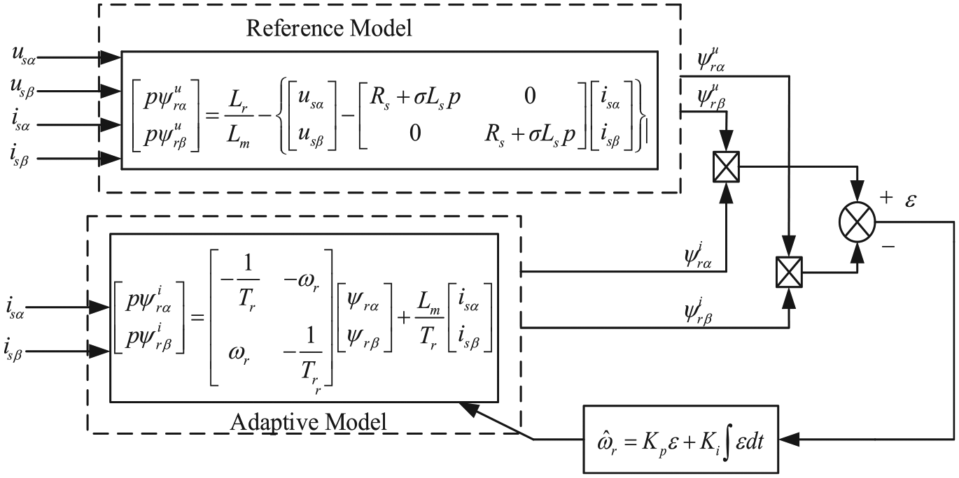
Based on the flux linkage, the principle of MRAS.
Rotor flux voltage model
Rotor flux current model

The adaptive law of estimating the rotational speed in accordance with the Popov’s stability theory 16 can be expressed as
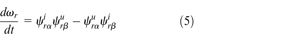
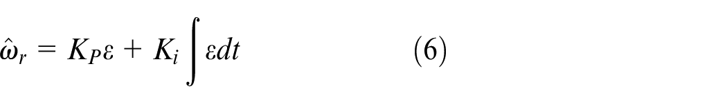
Let the estimated speed adaptation law be
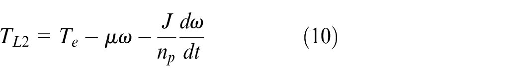
Load torque identification
In order to detect the anti-interference performance of the proposed method, the load torque is suddenly applied to the motor to observe the change of the speed. However, due to the unknown load torque, the torque is identified first

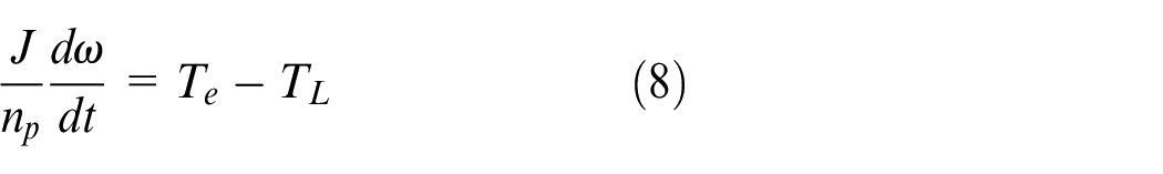
Motion equation of motion control system
Frictional resistance torque

Substituting equations (8) and (9) into equation (7), the following equation can be derived
where
According to the formula of speed identification, it could be concluded that the current model of the rotor flux linkage contains the speed information, and the voltage model is independent of the speed. Therefore, the MRAS system can be constructed, the voltage model can be selected as the reference model, the current model is used as adaptive model, estimating the generalized error of flux linkage is selected as the input of adaptive mechanism by voltage model and current model, and PI regulator is used as the adaptive mechanism to estimate the rotational speed. The output flux contains low frequency components and DC drift, due to the influence of pure integral in the voltage model. In order to solve this problem, the Butterworth filter is added to the system of speed estimation.
Design of Butterworth filter and MRAS based on SM observer
Design of Butterworth filter
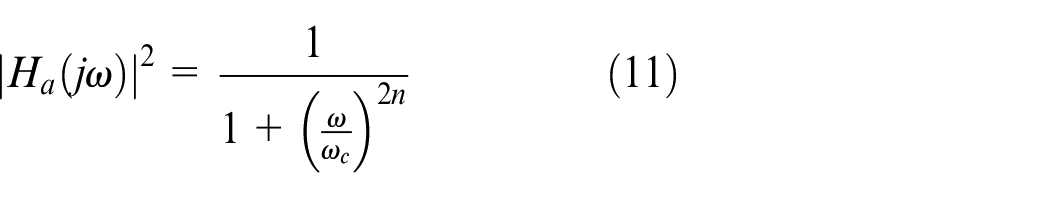
From the perspective of filter design, the designed filter needs to meet the actual demand as much as possible. The Butterworth filter has a monotonically decreasing amplitude–frequency characteristic. The frequency response curve in the passband is as flat as possible, with no undulations, and gradually decreases to zero in the blocking band. It can form four configurations of low pass, high pass, band pass, and band stop. It is the most popular type of digital filter at present, and can be used as digital Butterworth filter after discretization. Compared with analog filter, it has many advantages such as high accuracy, stability, flexibility, and no impedance matching. 17
As the filter order increases, the passband becomes flat, the transition zone decreases faster; hence, the error is smaller, but the amount of calculation increases greatly. In order to meet the actual demand, this paper uses the second-order Butterworth filter. The relationship between filter order and amplitude–frequency characteristics is as follows
where
Substituting
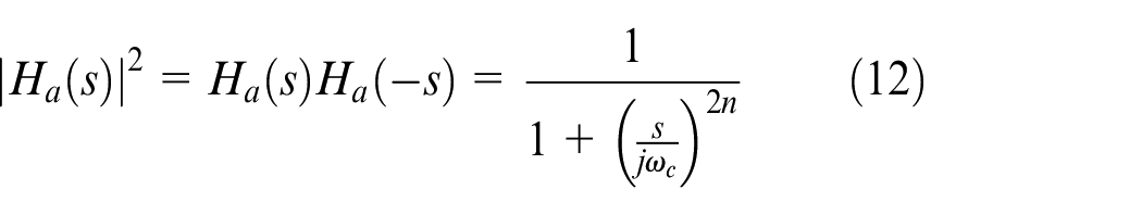
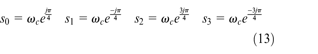
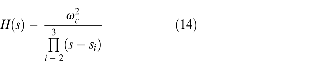
Since the filter requirements are designed to be achievable and stable, the pole in the left half plane is chosen as the pole
The cutoff frequency is taken as the standard frequency, and equation (14) is normalized
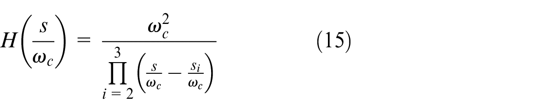
Substituting
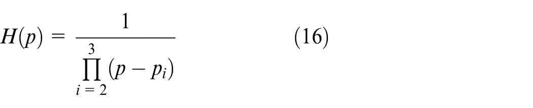
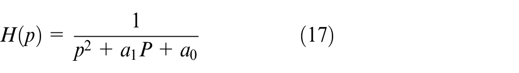
Substituting
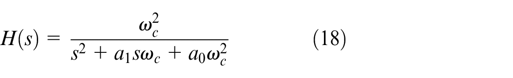
where
Figure 2 is the relationship between amplitude characteristics and order of Butterworth filter
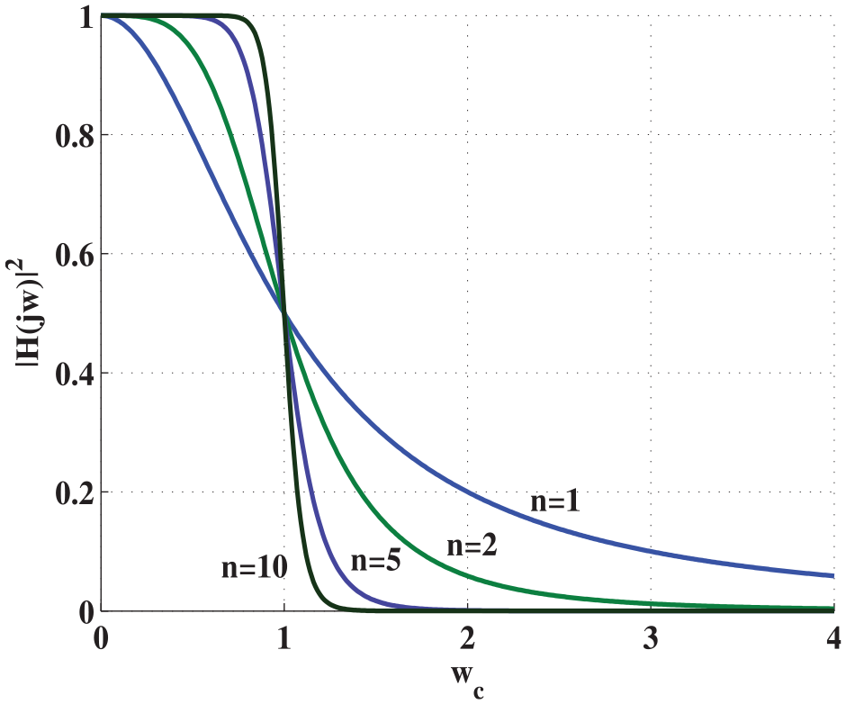
The relationship between amplitude characteristics and order of Butterworth filter
MRAS based on SM observer
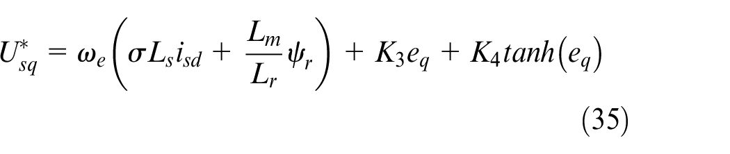
In order to further improve the robustness of the system, SM controllers are introduced to replace the traditional PI regulators, and the stability of the SM controllers is proved by Lyapunov theorem. SM control is widely used because of its good robustness to matching uncertainties. However, due to the existence of the symbol function, it can bring chattering problem to the system. In order to suppress this problem, the SM controllers are designed by the exponential approximation law, and the hyperbolic tangent function is used to replace the symbol function. The proposed controller is as follows

Proof of stability of formula (19). Define the sliding surface as
Its subdivision of time

It is known from the current model of the rotor flux linkage in the
Differential for
Substituting equation (22) into equation (23)
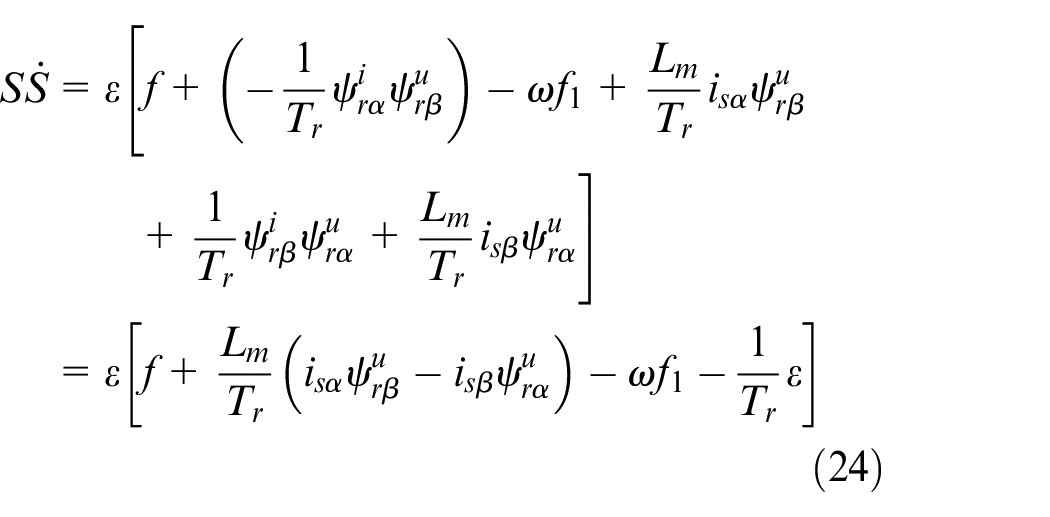
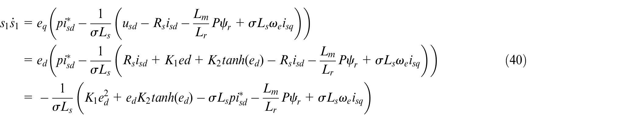
Substituting equation (19) into equation (24)
In equations (24) and (25)
Assume
Convergence analysis of SM state variables:
For a general system, its mathematical description is

There is a switching plane in its state space

Divide the state space into
Normal point—When the system moves to the vicinity of the switching plane
Starting point—When the system moves to the vicinity of the switching plane
End point—When the system moves to the vicinity of the switching plane
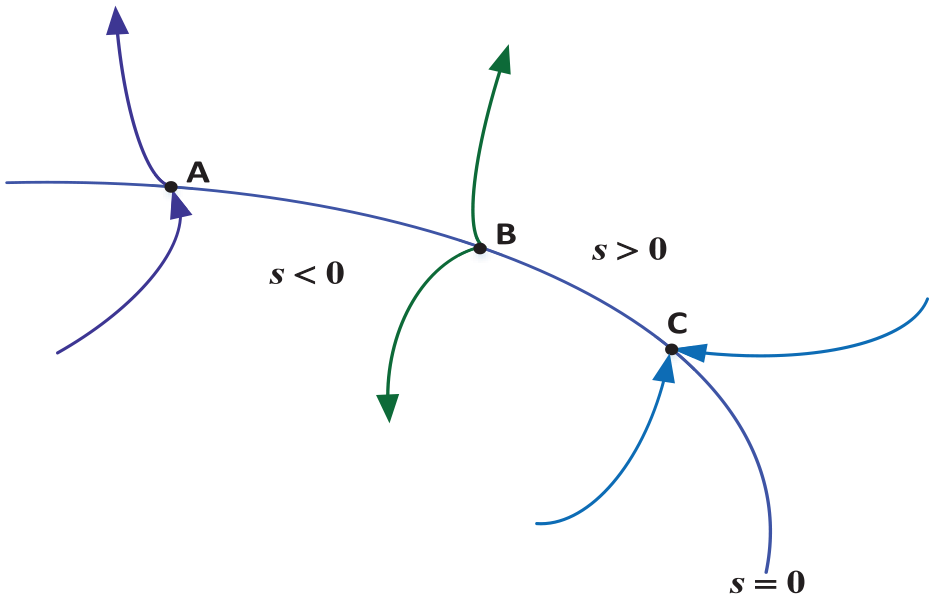
Switching characteristics of three points on the surface.
According to the requirement that the points on the SM area are the end points, when the moving point reaches the vicinity of the switching plane a = 0. Must have
Since the formula (31) in the switching plane is positive, according to the formula (30), the reciprocal of a is negative and semi-determined. That is to say, near
Figure 4 is the proposed method based on flux linkage speed estimation. The Butterworth filter is added to the speed estimation system. The simulation results show that the noise is eliminated. The conventional method obtains the values of the regulator parameters
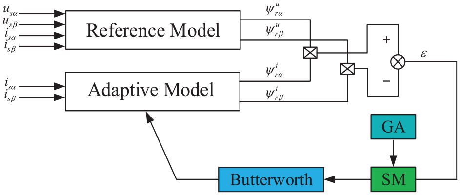
Schematic diagram based on flux linkage speed estimation.
Design of SM controller
SM variable structure
Variable structure control is a special kind of nonlinear control essentially, control discontinuity is the performance of variable structure control nonlinearity. This control strategy can be continually changed with the state of the system, causing the system to move according to a predetermined “SM” state trajectory. So, it is also called “SM variable structure control.” SM variable structure control is independent of system parameters and disturbances, which makes the variable structure control response speed and strong immunity. 21
Controller design
Traditional vector control system includes speed regulators, flux regulators, and two current regulators. In order to solve the problem of speed fluctuation in the speed estimation system, this paper adopts the control strategy combining fuzzy PI regulators and SM controllers. That is, the fuzzy PI regulators are used instead of the speed and flux regulators, and the SM controller replaces the current regulators. The current regulators proposed in this paper is as follows: the input of the SM current controllers is the difference between the given current and the feedback current of the rotor field oriented synchronous rotating coordinate system, and the output is command voltage.
Define the sliding surface as


where

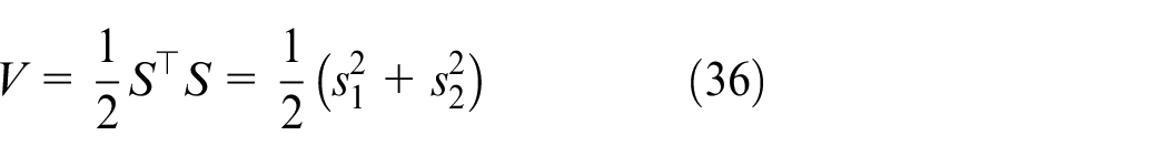
Proof of stability of formulas (34) and (35). Define the SM function as
Its subdivision of time

According to the rotor field orientation vector control system voltage equation can be obtained
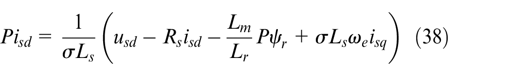
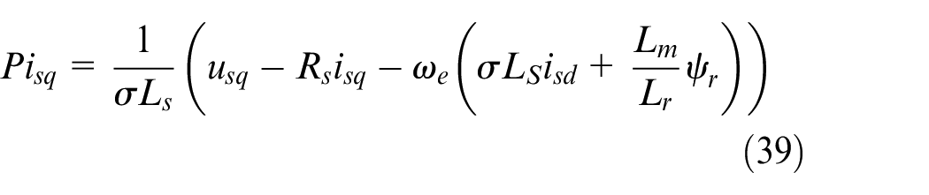
Substituting equations (38) and (39) into equation (37)
where p is the differential operator.
If
The system is stable as long as the parameters meet the requirements of equation (42). Replacing the current regulator with SM controller in a vector control system can effectively solve the problem of speed fluctuations. If the estimated speed is to track the actual speed to the maximum, the parameter selection of the controller is crucial. In order to obtain the optimal value of the estimated speed, the value of the SM controller parameters
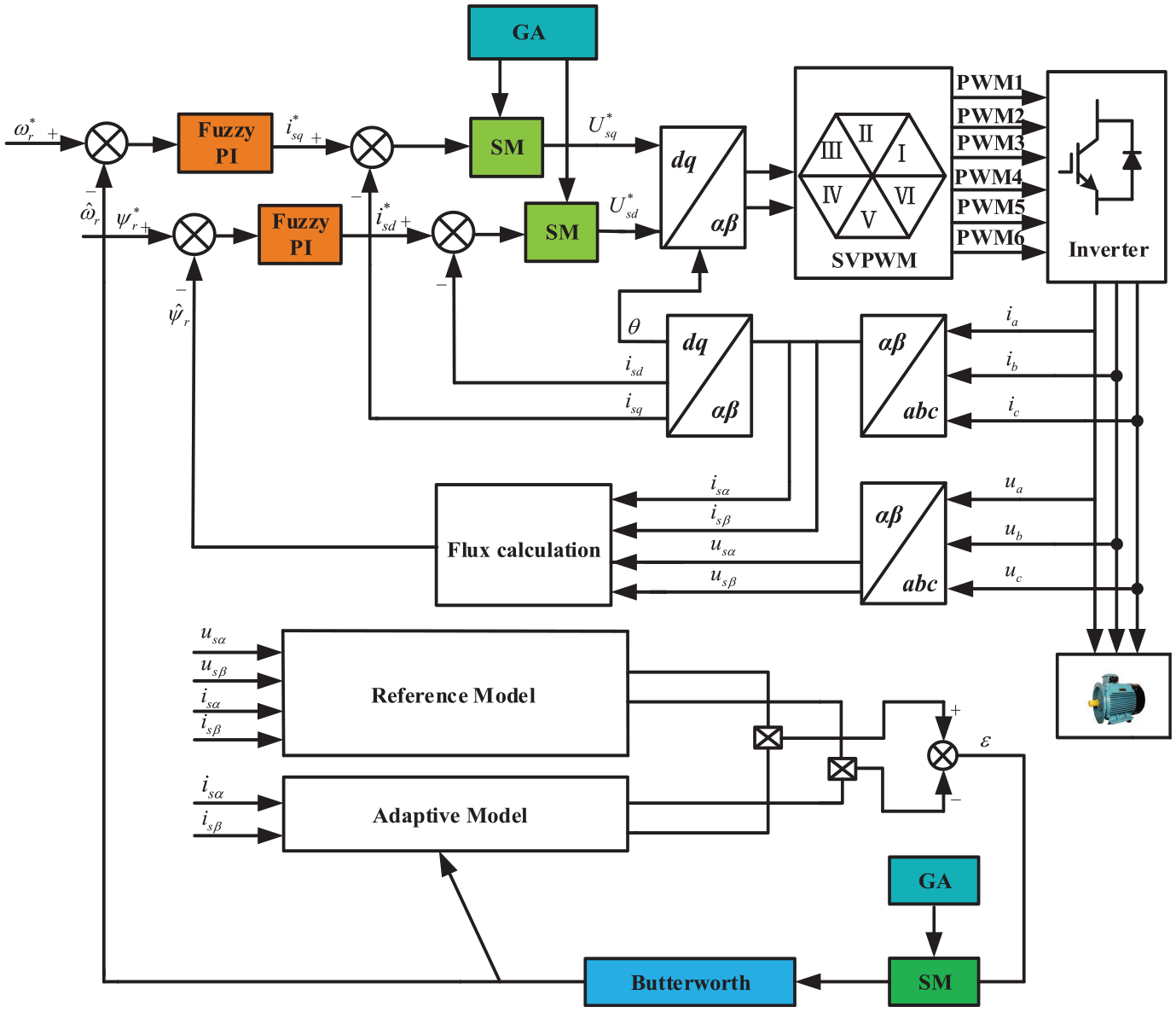
Improved vector control system diagram.
GA
GA originates from computer simulation studies of biological systems. In 1967, Bagley in the United States first proposed the term “genetic algorithm (GA).” GA is a random global search and optimization method that simulates the evolution of natural biological mechanisms. Using the principle of survival of the fittest, a new solution is generated every iteration. The iterative process will allow individuals in the population to evolve and produce new individuals that adapt to the environment better than the original individuals. 23 GA mimics the replication, crossover, and variation that occur in nature selection and inheritance. Starting from any initial populations, through random selection, crossover, and mutation operations, generate better individuals, and the population is evolved into a region with better and better search space. As the number of iterations increases, the most suitable individuals can be obtained. Thereby, the optimal solution is obtained. 24 However, standard GA cannot converge to global optimal value. In order to ensure its convergence, some improvements to the GA are needed. That is, the selection method does not select proportionally, but retains the current optimal value. The classical GA often uses the proportional selection method; the selection error of this selection method is relatively large; sometimes even individuals with higher fitness can’t choose. The GA that retains the current optimal value after selection can finally converge to the global optimal value. 25 In this paper, the GA is used to optimize the parameters of the three SM controllers simultaneously.
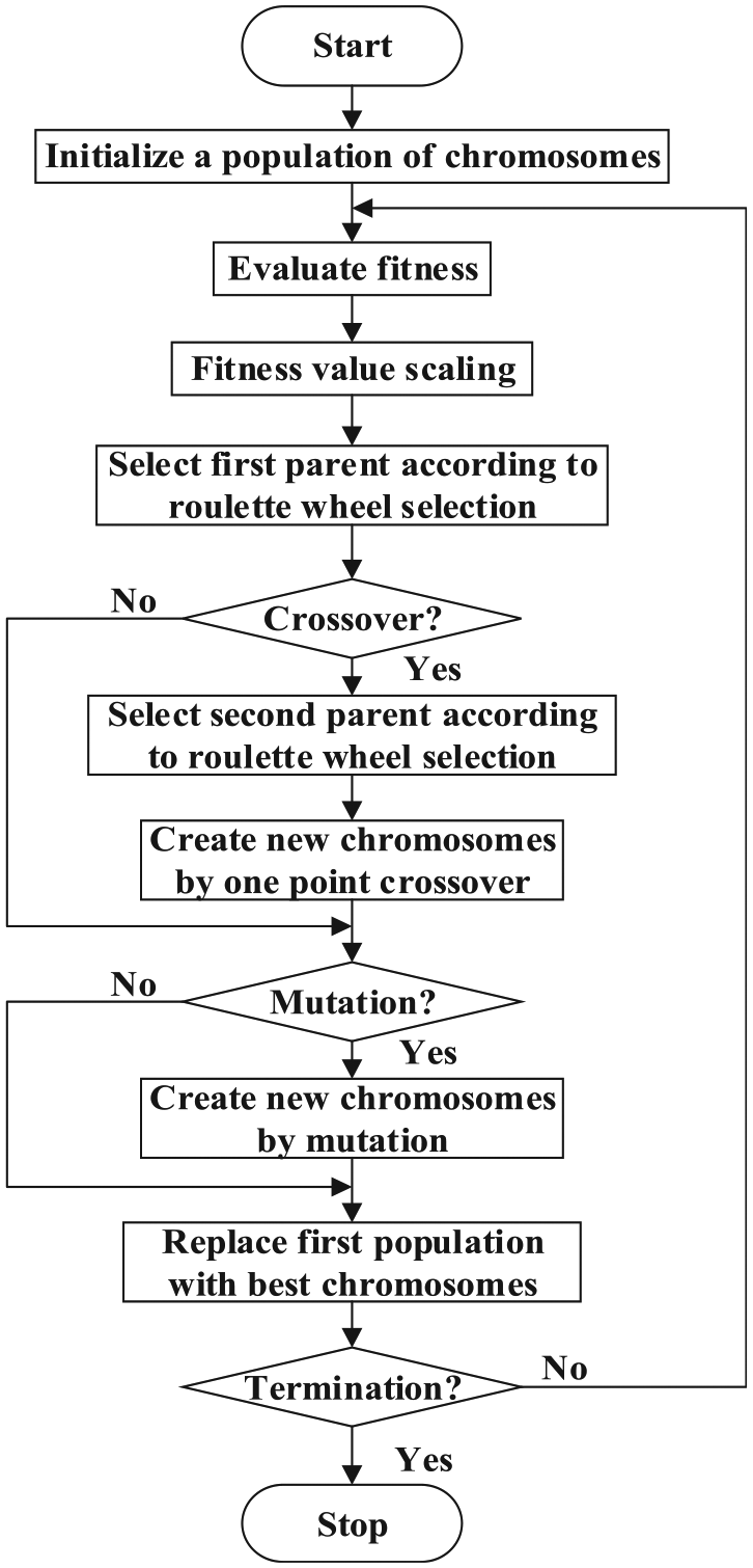
Define GA parameters. (Number of individual populations: 10, number of variables: 6, maximum genetic algebra: 10, binary digits of variables: 10, generation gap: 0.95, crossover probability: 0.7, and probability of variation: 0.01.) The specific operations are shown in Figure 6.
Schematic diagram based on flux linkage speed estimation.
When GA determines the parameters of the SM controllers, there must be a corresponding objective function that provide a method to measure the completion of the individual in the problem domain. For the optimization of controller parameters by GA, the selection of the objective function could affect the final optimization result directly. In order to enhance system performance and achieve optimal control, domestic and foreign scholars proposed various types of objective functions. Control system performance metrics are a measure of the good or bad of system performance. If a control system is at its best, it must have the best performance indicators. 26 Currently, there are three frequently used dynamic performance indicators as the following:
Excessive process quality indicators;
General functional integral index; and
Error functional integral index.
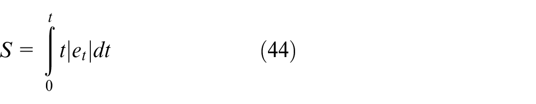
The error functional integral index measures whether a control system is in an optimal state by judging whether the objective function obtained a minimum value. It is simple to operate and easy to implement. Commonly used error functional integral indicators are ISTAE, ITAE, LAE, ISTSE, ITSE, and ISE. Integrated time absolute error (ITAE) criterion is a comprehensive index that can make the system own rapidity, accuracy, and stability. The control system designed according to this criterion has small transient response oscillation and good selectivity to parameters, which can achieve the purpose of eliminating the speed jitter and improving the dynamic performance of the system. Therefore, the ITAE is selected as the objective function of the GA optimization. Let the difference between the given current and the feedback current of the d-axis be

The expression of the objective function is
Simulation
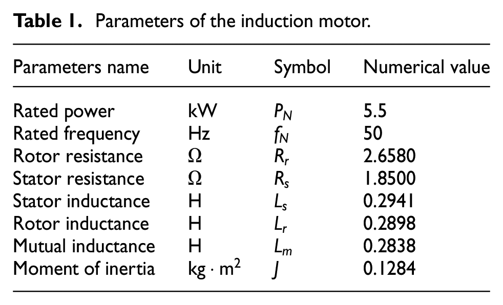
The simulation model is built under MATLAB/Simulink environment, which could verify the effectiveness of the proposed algorithm by comparing various parameters of the front and rear speed sensorless system. The selected motor parameters are shown in Table 1.
Parameters of the induction motor.
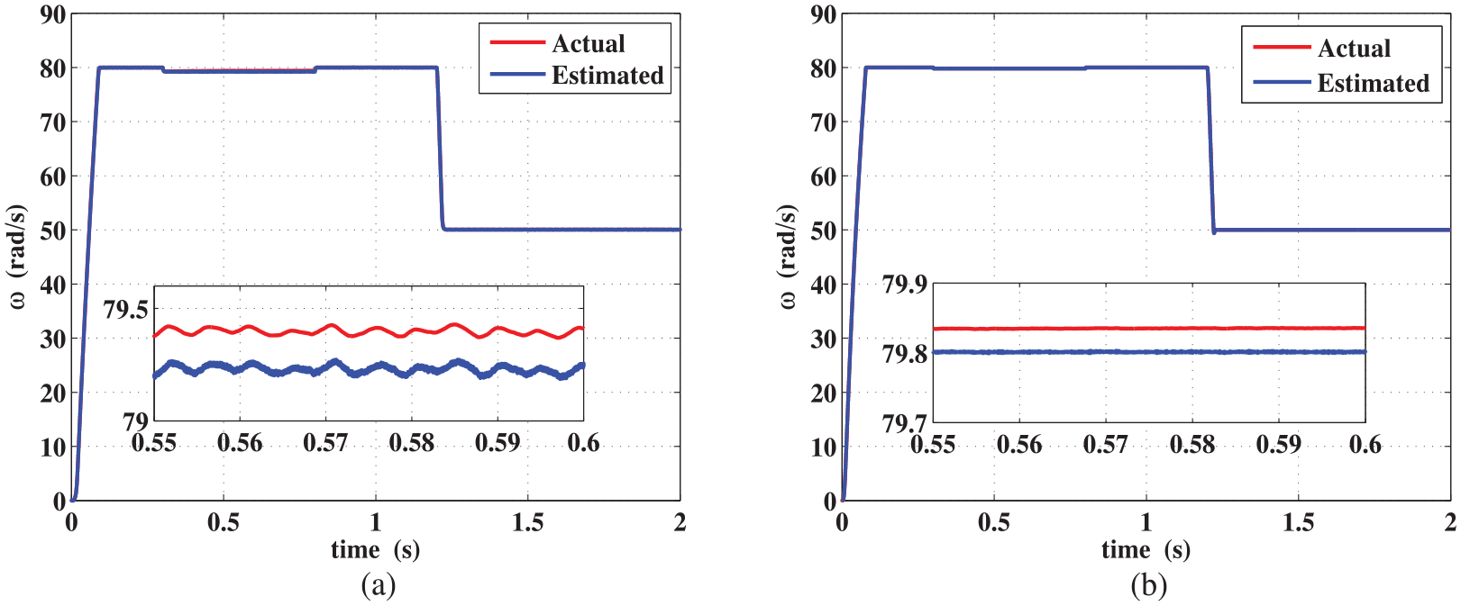
Simulation experiment results analysis is as follows: the simulation comparison of the flux model reference adaptive induction motor speed estimation system between the estimated speed before and after the improvement and the actual speed is shown in Figure 7(a) and (b). The initial speed is given as
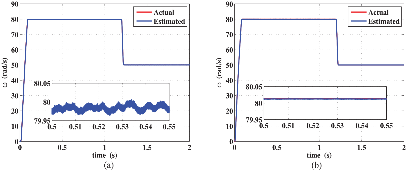
Estimated speed and actual speed before (a) and after improvement (b).
Due to the unknown load torque in actual conditions, the load torque is identified at first. Add
Estimated speed and actual speed before (a) and after improvement (b) (load).
This paper further illustrates the system tracking performance by calculating the relative error between the estimated speed and the actual speed before and after the improvement. The relative error calculation results are shown in Figure 9. Let the relative error value be equal to a. The relative error is divided into three levels: a < 0.05%, 0.05% ≤ a < 0.2%, and a > 0.2%. As can be seen from Figure 9(a), the data with a > 0.1% before the improvement account for about 1/2 of the total system data. As can be seen from Figure 9(b), about 2/3 of the data after the improvement are concentrated in the region where the relative error is a < 0.01%. It can be seen that the proposed method improves the system’s performance that estimated speed tracking actual speed.
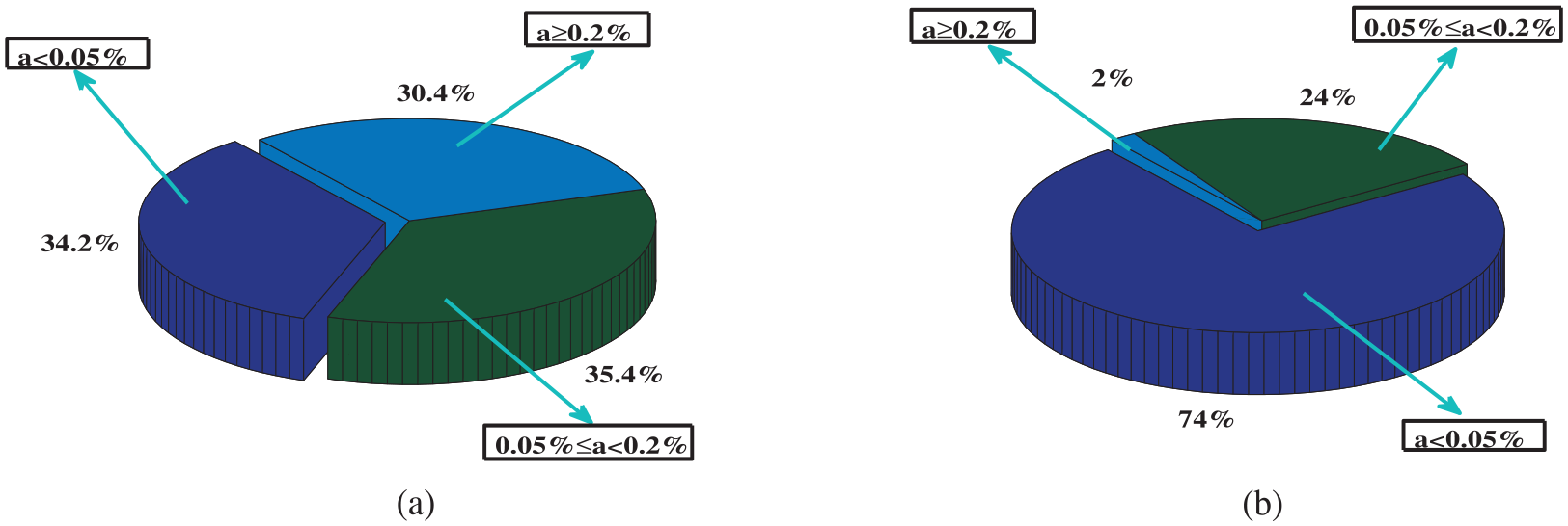
Actual speed and estimated speed relative error before (a) and after improvement (load) (b).
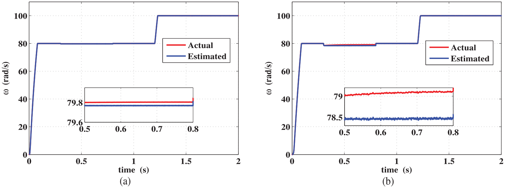
Due to the stator voltage error at low speed, the motor leads to unstable operation directly and low speed estimation accuracy; therefore, this is always a problem that has been caused by the induction motor speed sensorless system. Under the method proposed of this paper in the low speed state of the motor, the accuracy, immunity, and system dynamic performance are significantly improved. The initial speed is set to
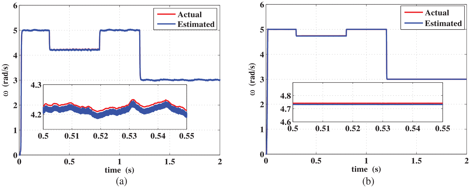
Estimated speed and actual speed before (a) and after improvement (b) (low speed, load).
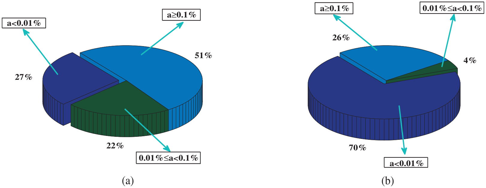
Actual speed and estimated speed relative error before (a) and after improvement (b) (low speed, load).
Figure 12(a) is a comparison of electromagnetic torque before and after improvement. It can be seen from the partial enlargement that there is a small amplitude fluctuation of the electromagnetic torque before the improvement, and the electromagnetic torque fluctuation after the improvement is basically eliminated.
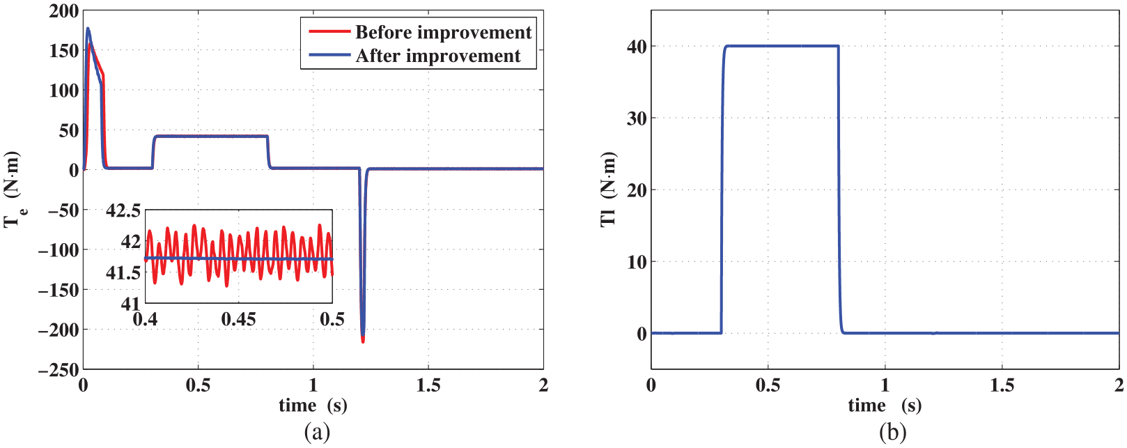
Electromagnetic torque before (a) and after improvement (b) and load torque identification.
Figure 13(a) is the tenth generation population distribution map. Figure 13(b) is the number of GA iterations and the optimal value of each generation. It can be seen from Figure 13(b) that the objective function value decreases with the increase in the number of iterations, and the last three generations of optimal values no longer change. In this paper, this value is taken as the optimal value of the objective function, and the variable values corresponding to the optimal values are taken as the controller parameters.
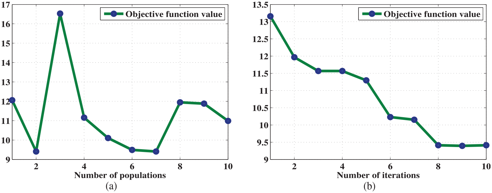
Iterative tenth objective function value distribution (a) and optimal value per generation (b).
The controller parameters corresponding to Figure 14(a) are determined by the GA, and the parameters corresponding to Figure 14(b) are determined by the particle swarm algorithm. It can be seen from Figure 14 that the parameters of controllers determined by the GA have higher accuracy of speed estimation.
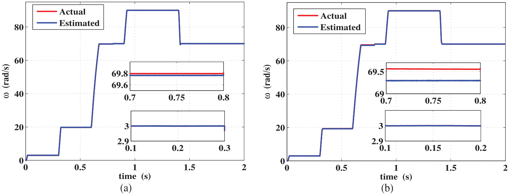
GA (a) and PSO (b) optimization results.
Figure 15(a) is a plot of the mean distribution of each generation of population; Figure 15(b) is the number of iterations of the particle swarm algorithm and the global optimal value corresponding to each generation. It can be seen from Figure 15(b) that the objective function value decreases as the number of iterations increases, and the last 14 generations of the optimal values no longer change. It can be seen from the figure that the optimal value of the objective function corresponding to the particle swarm optimization algorithm is larger than the optimal value corresponding to the GA, which further illustrates the superiority of the GA to such problems.
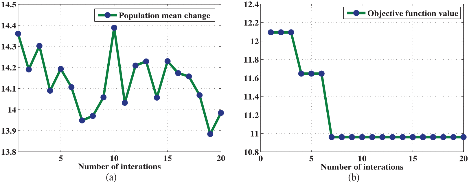
Particle swarm algorithm population mean change (a) and optimal value of each generation (b).
The control strategy corresponding to Figure 16(a) is combining fuzzy PI and SM, and the control strategy corresponding to Figure 16(b) is full fuzzy, that is, the fuzzy PI is used instead of the SM controller. Load disturbance is added at 0.3–0.8 s. It can be seen from Figure 16 that the fuzzy PI combined with the SM control strategy makes the system more robust and the speed estimation accuracy is higher.
Sliding mode controller (a) and fuzzy PI controller (b) comparison results.
Figures 17 and 18 are the comparison of the three-phase stator current before and after improvement. Figure 17 shows that the curve before the improvement is uneven, and the improved current curve is smoother and the shape tends to be more sinusoidal. At 1.2 s, the motor speed is adjusted, the amplitude of the change of the three-phase stator current is relatively large.
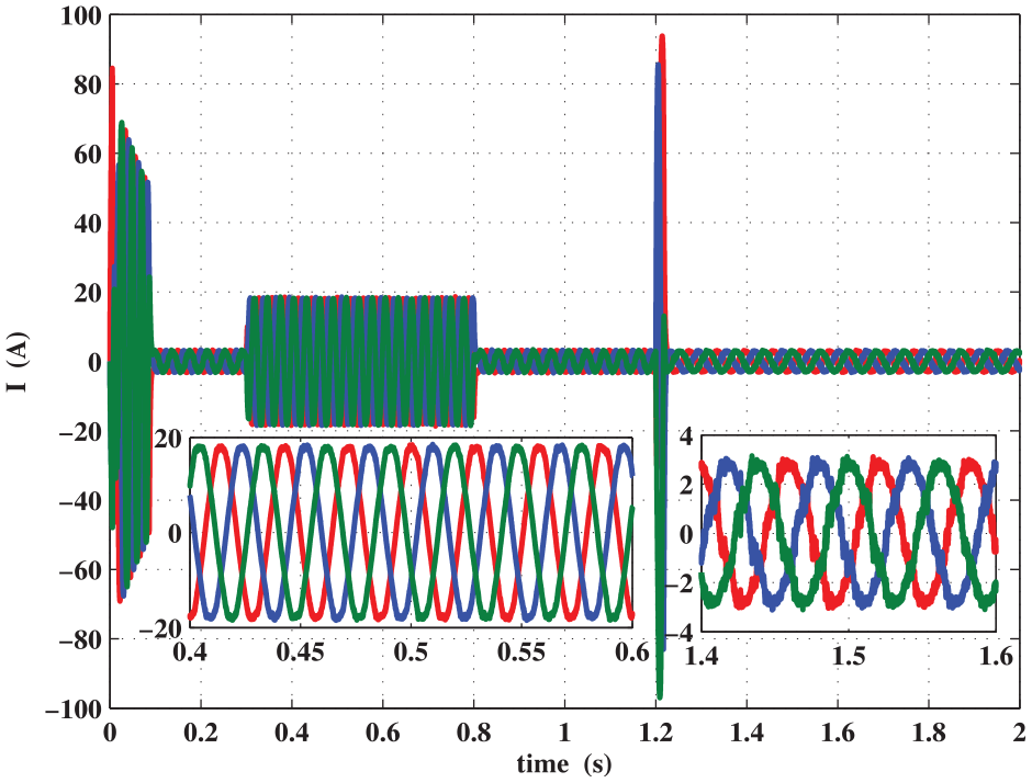
Before improvement three-phase stator current.
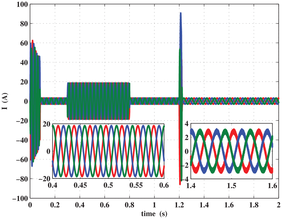
After improvement three-phase stator current.
Figure 19 is a comparison of the estimated rotational speed before and after the improvement with a given rotational speed. Among them, the load is added at 0.3–0.8 s. It can be seen from the partial enlargement diagram that the error between the estimated speed and the given speed is smaller after the improvement, and the noise and fluctuation are basically eliminated.
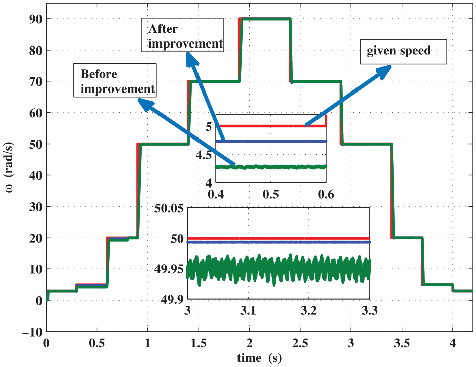
Reference speed and improved front and rear speed.
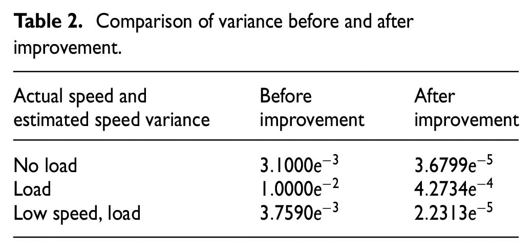
In order to further illustrate the superiority of the proposed method, the variance actual speed and estimated speed is compared. The result is shown in Table 2.
Comparison of variance before and after improvement.
Conclusion
In this paper, the motor speed is estimated based on the flux linkage model reference adaptive method. Due to the large number of high-order harmonics and noise in the voltage model and the existence of the speed fluctuation problem in the traditional vector control system, the speed estimation accuracy and system dynamic performance are seriously affected. By the introduction of Butterworth filters and fuzzy PI controllers, and according to Lyapunov’s stability theorem, SM controllers are designed to replace the current regulators of traditional vector control system and PI regulator of sensorless speed system. In order to obtain the optimal value of the speed estimation, the error integral criterion is adopted as the objective function, optimizing three SM controllers simultaneously using GA. The simulation results show that noise of system and speed fluctuations are basically eliminated, and speed estimation accuracy and dynamic performance are obviously improved.
The model reference adaptive speed sensorless vector control system directly affects the stability in the process of operation under the low speed range due to the stator voltage error. Moreover, the conventional speed estimation method has low precision in a low speed range, and it is difficult to achieve wide range speed regulation. In order to address the problem, the method proposed in this paper being applied in the low speed state of the motor, could the speed estimation accuracy and the anti-interference performance are greatly improved.
Footnotes
Declaration of conflicting interests
The author(s) declared no potential conflicts of interest with respect to the research, authorship, and/or publication of this article.
Funding
The author(s) received no financial support for the research, authorship, and/or publication of this article.