Sage Journals: Discover world-class research

Abstract

This paper presents a controller design method using lead and lag controllers for fractional-order control systems. In the presented method, it is aimed to minimize the error in the control system and to obtain controller parameters parametrically. The error occurring in the system can be minimized by integral performance criteria. The lead and lag controllers have three parameters that need to be calculated. These parameters can be determined by the simulation model created in the Matlab environment. In this study, the fractional-order system in the model was performed using Matsuda’s fourth-order integer approximation. In the optimization model, the error is minimized by using the integral performance criteria, and the controller parameters are obtained for the minimum error values. The results show that the presented method gives good step responses for lead and lag controllers.

Keywords

Controller design lead lag optimization

Introduction

Controller design is a common subject matter in the literature and there are many scientific studies in this regard. There are numerous studies on the design of proportional–integral–derivative (PID) controllers.^1–5 In this study, the design of a phase-lead and phase-lag controllers which are also commonly used in the control applications has been studied.

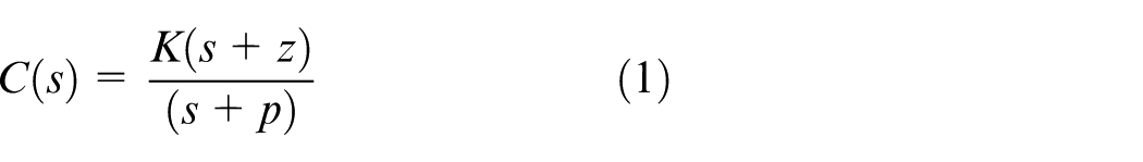
Lead and lag controllers are mostly used in industrial servo systems with integral effect and have better control performance than PID controllers. Although the lead and lag controllers are similar in general structure, they differ in terms of the location of poles and zeros. While the lead controller provides phase progression to the system, the lag controller acts as a phase regression. The lead controller is preferred if a fast response is desired in the system, and the lag controller is used if it is desired to improve the steady state accuracy. A good control system needs to meet required specifications. The time domain parameters and percent overshoot value in the transient state behavior are important for monitoring the performance of the control system. A phase-lead controller improves the time response of the system such as reducing the percent overshoot value. In addition, it allows the system to respond faster by increasing the gain crossover-frequency and bandwidth of the system. The phase-lag controller causes the time parameters to lengthen, while reducing the percent overshoot. As a result, the response time of the system decreases.⁶ The controller structure used in the study is given in Equation (1). In Equation (1), if z < p, then the controller is phase-lead, and if z > p, then the controller is called as phase-lag controller. There are three parameters that must be determined in the controller structure. These parameters can be determined using the optimization method

C (s) = \frac{K (s + z)}{(s + p)}

(1)

The interest in fast, easy and successful determination of controller parameters increases day by day. Although there are many tuning methods in determining the parameters of PID controllers, there are limited tuning methods available in lead and lag controllers. The root locus and Bode diagram approach are two most commonly used methods for designing control systems with the phase-lead and phase-lag controller.

Loh et al.⁷ developed an online algorithm based on a hysteresis relay to determine lead and lag controller parameters. Yeung and Lee⁸ developed a design chart method for the phase-lead and phase-lag controllers. The tuning methods of Ogata and Yang⁶ have been applied widely in the design of lead and lag controllers. It is a method based on a trial and error; therefore, both the gain and phase margin specifications may not be satisfied very well. With the advances in computer and software development as well as optimization algorithms, controller parameters are determined quickly and successfully. Optimization is described as a systematic problem-solving process performed by placing values into the function to minimize or maximize a real function.⁹ It is used in determining the controller parameters as well as heuristic algorithms and Matlab-based algorithms. In his study, Horng¹⁰ successfully performed the lead–lag controller designs according to the desired time responses using the genetic algorithm (GA). The examples presented in his study are for integer-order plants. Monje et al.¹¹ proposed an auto-tuning method for controlling integer-order systems using a fractional-order lead/lag controller. Yeroglu and Tan¹² determined lag and lag–lead controller parameters by using classical design methods with Bode envelopes for fractional-order interval transfer function. In the Salehtavazoei and Tavakoli-Kakhki¹³ study, they presented a method for performing a fractional-order lead/lag controller design according to the desired gain and phase margin for a given frequency for the integer-order system. Khiabani and Babazadeh¹⁴ conducted a robust fractional-order lead–lag controller design for uncertain and integer-order systems. In literature, it is seen that the use of lead and lag controller is limited in fractional-order systems.

In control systems, the error is expressed as the difference between the actual and the desired value of the system.¹⁵ In an idealized system, the error is considered to be zero. The control system is required to follow the signal applied to the input. In practice, this is not possible and an error occurs. Minimizing the error will enable the control system work at optimal performance. Optimization technique is utilized for error minimization. This technique uses integral performance criteria to minimize the error. The controller is designed on the basis of the controller parameters that guarantee minimum error.

The important contribution of this study is the use of fractional-order control systems. Studies on the fractional-order calculation have a history of three centuries. Applications in science and engineering are increasing rapidly in line with the advances in computational techniques.¹⁶ In the literature, there are numerous studies on the development of integer-order approximations of fractional-order integral and derivative in order to apply classical control design approaches. The most important of these are the Matsuda and Fujii,¹⁷ Oustaloup et al.¹⁸ and Carlson and Halijak¹⁹ integer approximation methods. Yin et al.²⁰ have been investigated the robust stability analysis for fractional-order singular nonlinear system with the fractional-order proportional derivative (PD) controller. In their study, Luo et al.²¹ have successfully performed fractional-order control systems with fractional-order PID controller. Hamamci²² presented a stabilization method to obtain the stabilizing fractional-order PID controllers for a given fractional-order time delay system. Yin et al.²³ proposed a fractional-order sliding mode controller technique and a fractional-order proportional integral (PI) controller design for robust stabilization of uncertain fractional-order nonlinear systems. Zhao et al.²⁴ proposed a method for fractional-order PID controller design for fractional-order systems. They emphasized that fractional-order models are becoming increasingly important for real processes. It is understood from the above-mentioned studies how important it is to quickly and successfully determine the controller parameters by using optimization methods for fractional-order systems.

The remainder of the paper is concerted as follows. The fundamentals of fractional calculus in control systems is described in “Fundamentals of fractional-order systems and stability analysis” section. In this section, some definitions related to stability analysis of fractional-order systems have been given. “Integral performance criteria and optimization method” section provides information on the integral performance criteria used in optimization. “Implementation of the optimization method” section presented with the implementation of the optimization method used to design phase-lead and phase-lag controllers. Conclusions are given in the last section.

Fundamentals of fractional-order systems and stability analysis

Fractional calculus is a branch of mathematics and has a history of 300 years. Fractional-order mathematics is related to non-integer derivatives and integrals. The fractional-order mathematics has been discussed in the correspondence between Leibniz and L’Hospital in 1695. The first theoretical studies in this area have been made by Euler and Lagrange in the 18th century. In addition, first methodical studies have been made by Liouville, Riemann and Holmgren in the 19th century. Abel presented the first application related to fractional calculus in 1823. Abel found that the solution could be accomplished via an integral transform for tautochrone problem.²⁵ Engineering applications of fractional calculus in the field of feedback control, systems theory and signal processing has a history of 50 years.⁴,²⁶ The position control was studied in 1958 by Tustin et al.²⁷ Manabe²⁸,²⁹ contributed to this topic with his studies. He used fractional integrator in his studies.

At first, there are limited number of applications because of the computational difficulties. In parallel with developments in computer technology, studies in recent years have increased rapidly. Fractional-order calculations have become quite popular in recent years. During this period, many applications were made by scientists and engineers in different areas.¹⁶

Fractional calculus is the generalization of integration and differentiation. Fractional-order fundamental operator ${{}_{a}D}_{t}^{α}$ is defined as in Equation (2) where a and t are the limits and α is the order of the operation²⁶,³⁰,³¹

{{}_{a}D}_{t}^{α} = {\begin{matrix} \frac{d^{α}}{d t^{α}}; α > 0 \\ 1; α = 1 \\ \int_{a}^{t} {(d τ)}^{- α}; α < 0 \end{matrix}

(2)

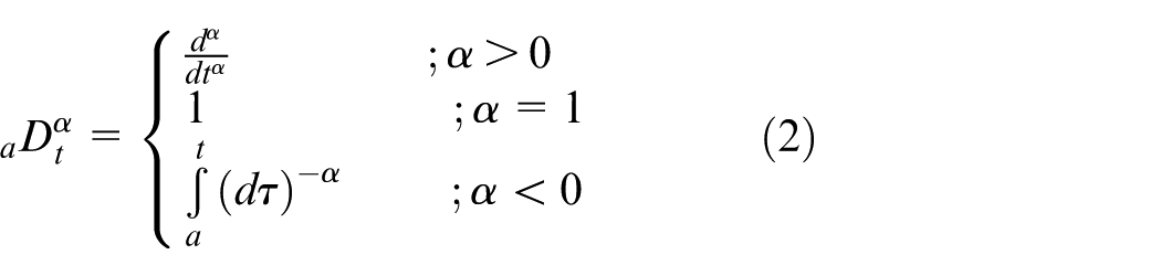
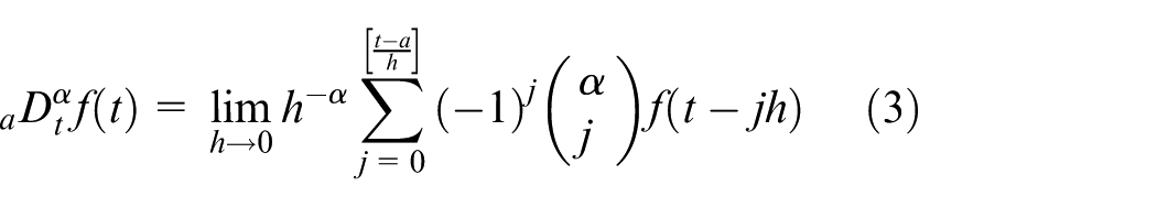
There are many definitions used for fractional-order integral and derivative, and the two most famous are Grünwald–Letnikov and Riemann–Liouville. The Grünwald–Letnikov definition is given as in Equation (3)²⁶,³⁰,³¹

{{}_{a}D}_{t}^{α} f (t) = lim_{h \to 0} h^{- α} \sum_{j = 0}^{[\frac{t - a}{h}]} {(- 1)}^{j} (\begin{matrix} α \\ j \end{matrix}) f (t - jh)

(3)

where $(- 1)^{j} (\begin{matrix} α \\ j \end{matrix})$ is binomial expansion coefficients.

The Riemann–Liouville definition is given as in Equation (4)

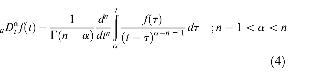
{{}_{a}D}_{t}^{α} f (t) = \frac{1}{Γ (n - α)} \frac{d^{n}}{d t^{n}} \int_{α}^{t} \frac{f (τ)}{{(t - τ)}^{α - n + 1}} d τ; n - 1 < α < n

(4)

where Г is the Gamma function.

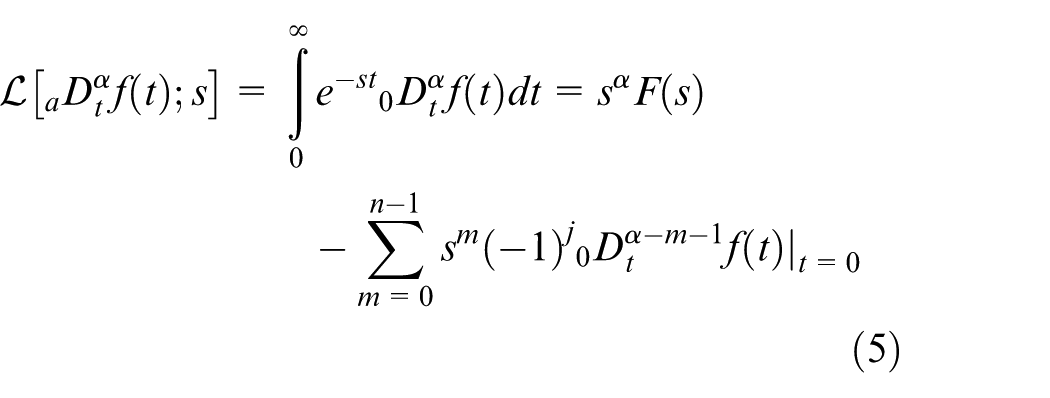
The Laplace transform of the fractional integral and derivative of Grünwald–Letnikov and Riemann–Liouville is defined as in Equation (5)

\begin{matrix} L [{{}_{a}D}_{t}^{α} f (t); s] = \int_{0}^{\infty} e^{- st} {{}_{0}D}_{t}^{α} f (t) dt = s^{α} F (s) \\ - \sum_{m = 0}^{n - 1} s^{m} {(- 1)}^{j} {{}_{0}D}_{t}^{α - m - 1} {f (t) |}_{t = 0} \end{matrix}

(5)

A fractional-order dynamical system can be described by a fractional-order differential equation

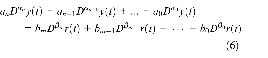
\begin{matrix} a_{n} D^{α_{n}} y (t) + a_{n - 1} D^{α_{n - 1}} y (t) + . . . + a_{0} D^{α_{0}} y (t) \\ = b_{m} D^{β_{m}} r (t) + b_{m - 1} D^{β_{m - 1}} r (t) + \dots + b_{0} D^{β_{0}} r (t) \end{matrix}

(6)

where r(t) is the input signal, y(t) is the output signal, $D^{γ} \equiv {{}_{0}D}_{t}^{γ}$ represents fractional derivative, $a_{k} (k = 0, . ., n)$ and $b_{k} (k = 0, . ., m)$ denote constants, and $α_{k} (k = 0, \dots, n)$ and $β_{k} (k = 0, . ., m)$ are arbitrary real numbers.²⁶,³⁰,³¹

Equation (6) can be expressed in terms of a transfer function as

G (s) = \frac{Y (s)}{R (s)} = \frac{b_{m} s^{β_{m}} + b_{m - 1} s^{β_{m - 1}} + \dots + b_{0} s^{β_{0}}}{a_{n} s^{α_{n}} + a_{n - 1} s^{α_{n - 1}} + \dots + a_{0} s^{α_{0}}}

(7)

It is very important to analyze the stability of the control systems. The system is stable if the roots of the characteristic equation of an integer-order system (Linear Time Invariant (LTI)) are located on the left half plane of the complex plane.⁶ Stability analysis in fractional-order systems differs from integer-order systems. A stable fractional-order system may have roots on the right half of the complex plane. The Routh–Hurwitz criterion, the Nyquist stability criterion or root locus method used in the stability analysis of integer-order systems cannot be applied directly to fractional-order systems. Instead, geometric techniques of complex analysis based on the argument principle are used. There are some studies in the literature on stability analysis of fractional-order systems.^32–36 The Matignon stability theory can be used in the stability analysis of fractional-order control systems.^37–39 The state-space model of a fractional-order LTI system is given in Equation (8)

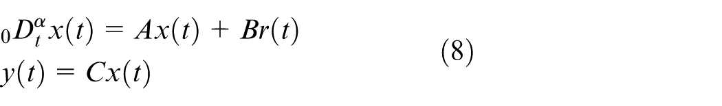
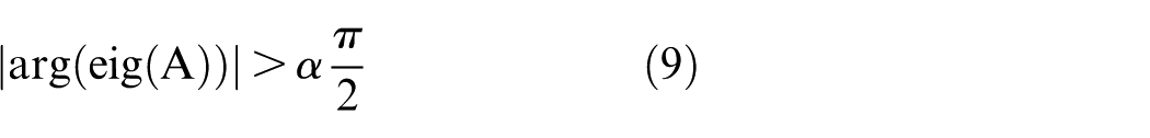
\begin{matrix} {{}_{0}D}_{t}^{α} x (t) = Ax (t) + Br (t) \\ y (t) = Cx (t) \end{matrix}

(8)

Here, α indicates the order of fractional-order system. Also, xϵRⁿ, rϵR^r and yϵR^p indicate the state, input and output vectors of the system, respectively. In addition, A ϵR^nxn, B ϵR^nxr and C ϵR^pxn, respectively, refer to the state, input and output matrix of the system. In order for the system given in Equation (8) to be stable, it must satisfy the condition given by Equation (9)⁴⁰,⁴¹

| \arg (eig (A)) | > α \frac{π}{2}

(9)

For a system given in Equation (10), the system becomes stable if the condition in Equation (11) is met⁴⁰,⁴¹

G (s) = \frac{Z (s)}{P (s)}

(10)

| \arg (w) | > α \frac{π}{2}, \forall w \in C, P (w) = 0

(11)

It is defined here as w = s^α. If w = 0, the P(s) polynomial has one root and the system is unstable. If α = 1, the system becomes integer-order system. Therefore, stability analysis is performed as in integer-order systems.

Figure 1 shows the regions of the complex plane which are stable and unstable for fractional-order systems.

Figure 1.

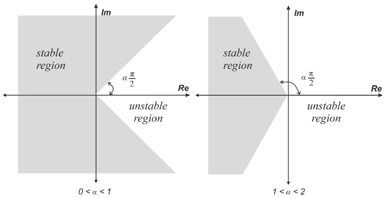
Stability region of the fractional-order system.

An analysis of the stability for a fractional-order plant given in Equation (12) was performed as follows

G (s) = \frac{K}{s^{1 + α} (Ts + 1)}

(12)

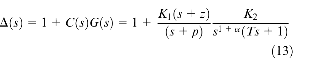
The characteristic polynomial of the controlled system is written in Equation (13)

Δ (s) = 1 + C (s) G (s) = 1 + \frac{K_{1} (s + z)}{(s + p)} \frac{K_{2}}{s^{1 + α} (Ts + 1)}

(13)

Δ (s) = s^{1 + α} (T s^{2} + (1 + Tp) s + p) + K_{1} K_{2} (s + z)

(14)

\begin{matrix} Δ (s) = T s^{3 + α} + (1 + Tp) s^{2 + α} + p s^{1 + α} \\ + K_{1} K_{2} s^{1} + K_{1} K_{2} z \end{matrix}

(15)

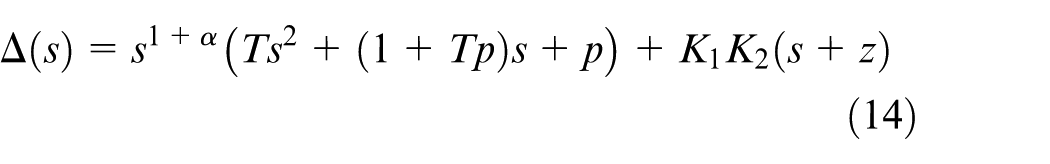
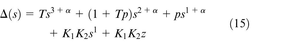
The characteristic polynomial is found in Equation (16), with mathematical operations performed as in Equations (14) and (15)

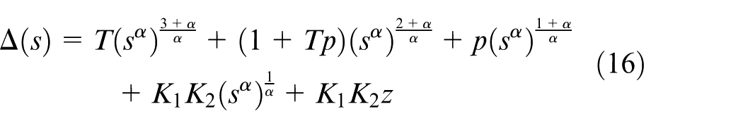
\begin{matrix} Δ (s) = T {(s^{α})}^{\frac{3 + α}{α}} + (1 + Tp) {(s^{α})}^{\frac{2 + α}{α}} + p {(s^{α})}^{\frac{1 + α}{α}} \\ + K_{1} K_{2} {(s^{α})}^{\frac{1}{α}} + K_{1} K_{2} z \end{matrix}

(16)

For $w = s^{α}$ , the equation is written as Equation (17)

\begin{matrix} Δ (w) = T {(w)}^{\frac{3 + α}{α}} + (1 + Tp) {(w)}^{\frac{2 + α}{α}} + p {(w)}^{\frac{1 + α}{α}} \\ + K_{1} K_{2} {(w)}^{\frac{1}{α}} + K_{1} K_{2} z \end{matrix}

(17)

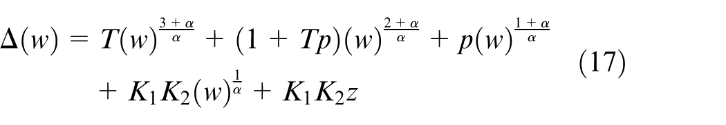
If the obtained equation is equal to zero and resolved, the roots of the characteristic polynomial are obtained. Thus, stability analysis is performed by placing roots on the complex plane.

Integral performance criteria and optimization method

The performance of control systems is usually assessed in terms of transient behavior. Parameters such as percent overshoot, rise and settling time are desired to be low. Controller design is important in order to get desired parameters of transient behavior. Optimization methods can be used to design the best controller for the system. Optimization is the process of choosing the best under certain conditions. In the optimization method, integral performance criteria are used to minimize the error in the control system. The error is known as the difference between the input and the output in a simple control system and is described by Equation (18)¹⁵

e (t) = r (t) - y (t)

(18)

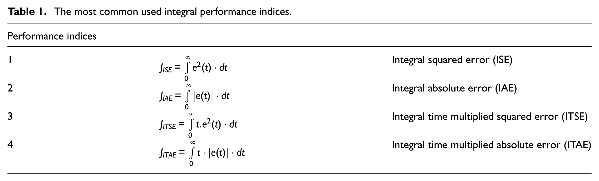
In the literature, there are four integral performance criteria commonly used, and are shown in Table 1.¹⁵,⁴² In the fourth section, for example, models were created using each performance criterion and the controllers were designed.

Table 1.

The most common used integral performance indices.

Performance indices
1	$J_{ISE} = \int_{0}^{\infty} e^{2} (t) \cdot dt$	Integral squared error (ISE)
2	$J_{IAE} = \int_{0}^{\infty} \| e (t) \| \cdot dt$	Integral absolute error (IAE)
3	$J_{ITSE} = \int_{0}^{\infty} t . e^{2} (t) \cdot dt$	Integral time multiplied squared error (ITSE)
4	$J_{ITAE} = \int_{0}^{\infty} t \cdot \| e (t) \| \cdot dt$	Integral time multiplied absolute error (ITAE)

There are commands that can be used for minimization or maximization in the Matlab Optimization Toolbox. Fminsearch, fmincon, fsolve and GA are some of them. The fmincon function in MATLAB software is used for optimization. The fmincon function finds the minimum values of the constrained nonlinear multivariable function.⁴³

For optimization, a model was created in the Matlab Simulink environment. The block diagram used in the design is shown in Figure 2.

Figure 2.

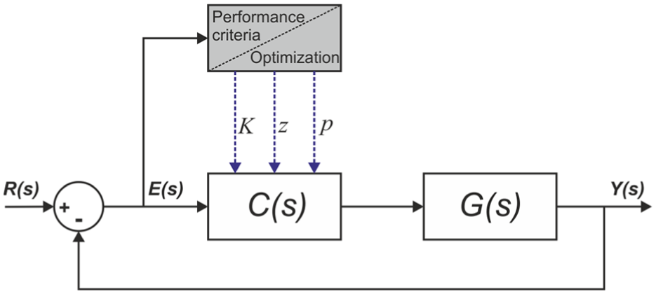
The block diagram of the given design method.

The controller design procedure is as follows:

Step 1: First, the model and objective function of the control system are created.

Step 2: Fmincon implements four different algorithms. Here, we choose to use interior point algorithm.

Step 3: The lower and upper bounds (lb and ub) on the design variables are defined.

Step 4: Initial values are entered in the control parameters.

Step 5: The optimization is run and the Fmincon algorithm calculates the minimum value for the objective function using Equation (19)⁴³

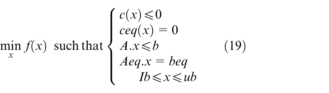
\min_{x} f (x) such that {\begin{matrix} c (x) \leq 0 \\ ceq (x) = 0 \\ A . x \leq b \\ Aeq . x = beq \\ Ib \leq x \leq ub \end{matrix}

(19)

where c(x) and ceq(x) are functions that return vectors, b and beq are vectors, A and Aeq are matrices, f(x) is a function, and x, lb and ub can be passed as vectors or matrices.

Step 6: The optimization algorithm stops at the end of certain iteration or when the desired fitness value is provided. If the required fitness value is not achieved, Step 2 is repeated.

Implementation of the optimization method

In this section, four examples of how to implement the lag and lead controllers design are presented. In the simulation model in the examples, the fractional-order system was performed with Matsuda’s integer-order approximation (Appendix I).

Example 1

Consider the system with the transfer function given in Equation (20)

G_{p 1} (s) = \frac{2}{s^{1.2} (1 + 0.5 s) (1 + 0.3 s)}

(20)

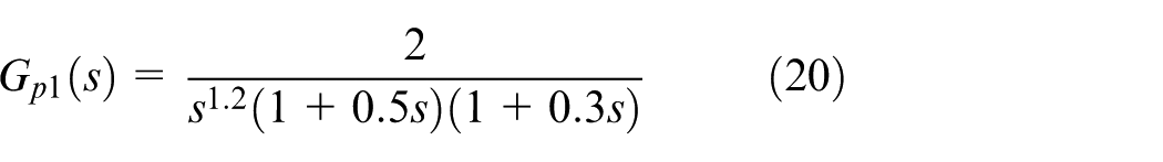
Closed-loop unit-step response of the fractional-order control system with C(s) = 1 is demonstrated in Figure 3. A model representing the fractional-order system was constructed in the Matlab/Simulink environment for integral performance criteria. Figure 4 shows the model based on integral time multiplied absolute error (ITAE) criterion.

Figure 3.

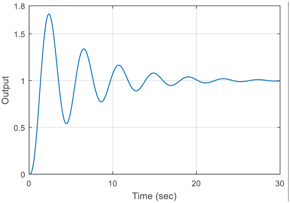
Step response of the closed loop system with C(s) = 1 and G_p₁(s) of Equation (20).

Figure 4.

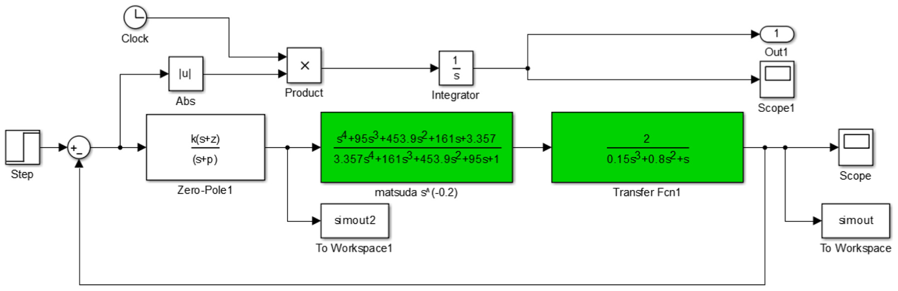
Simulink model with ITAE.

The controller parameters are determined by running the optimization. The phase-lead controller parameters are shown in Table 2 that it is performed for different performance criteria. Similarly, phase-lag control parameters are obtained and are presented in Table 2. For this example, in order to design phase-lag controller, the range for z was taken as [8.2, 20] and for p was taken as [0.1, 8] for optimization. From Table 2, it can be seen that all optimization criteria give same results for z and p in case of phase-lag controller. When we choose different range for parameters than the optimization block, it resulted in phase-lead controller.

Table 2.

The lead and lag controller parameters.

	IAE	ISE	ITSE	ITAE
Lead
K	20	20	20	14.6214
z	0.6738	0.4148	0.6344	0.8253
p	19.5045	13.2105	17.6377	20
Lag
K	0.46	0.54	0.44	0.39
z	8.2	8.2	8.2	8.2
p	8	8	8	8

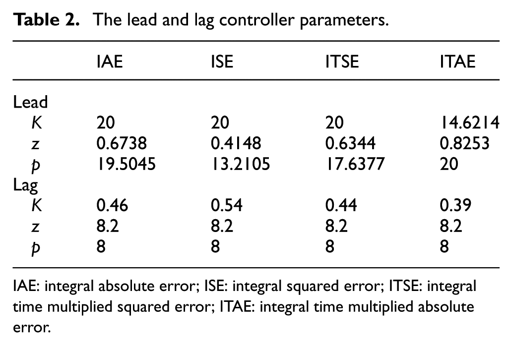
IAE: integral absolute error; ISE: integral squared error; ITSE: integral time multiplied squared error; ITAE: integral time multiplied absolute error.

The phase-lead and phase-lag controllers are determined by replacing the controller parameters in Table 2 in Equation (1). Figure 5 demonstrates the step responses for phase-lead controllers. Similarly, the step responses given in Figure 6 are obtained by applying the phase-lag controller to the closed loop system.

Figure 5.

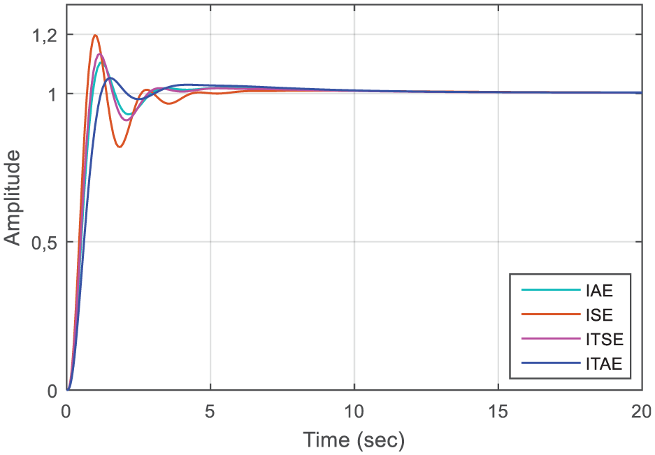
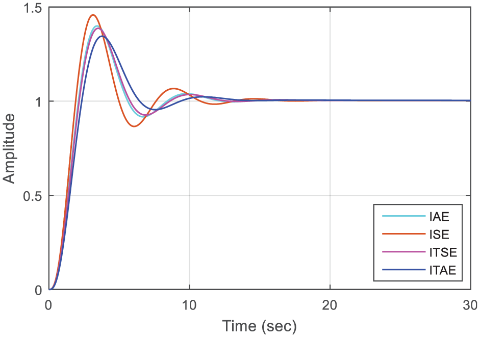
Step responses for G_p₁(s) with phase-lead controllers.

Figure 6.

Step responses for G_p₁(s) with phase-lag controllers.

Although the percent overshoot of the system without controller was 71.72%, it decreases to 4.87% when controlled by the phase-lead controller. Similarly, when controlled with a phase-lag controller, it drops to 33.96%. The ITAE criterion provides the lowest value in percent overshoot value.

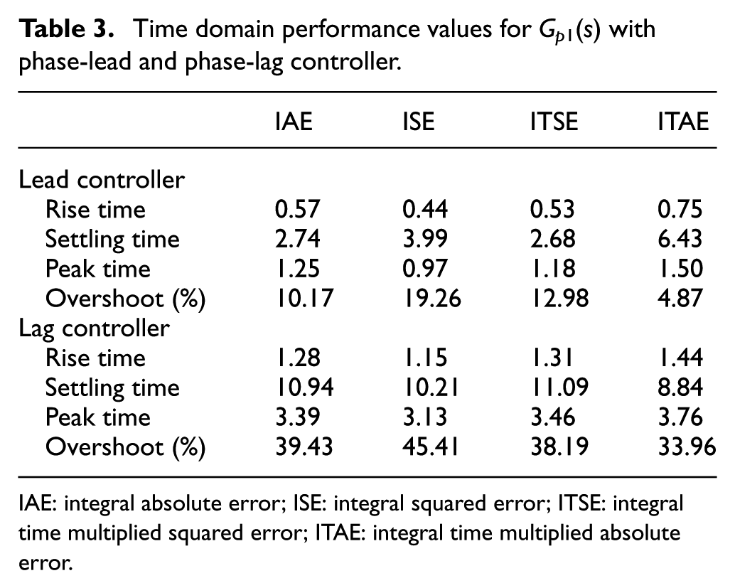
Time domain performance specifications for the first example are presented in the Table 3. The settling time of the system dropped from 23.61 to 2.68 s when controlled with the phase-lead controller. Here, the lowest settling time was provided by the integral time multiplied squared error (ITSE) criterion. In the system controlled by the phase-lag controller, the minimum settling time obtained was 8.84 s with the ITAE performance criterion. It is noteworthy that the times are significantly shorter in other time parameters as well. When the integral squared error (ISE) criterion is considered, while the system’s peak time is about 0.97 s with the lead controller, it extends with lag controller to 3.13 s. There is no doubt that the lead controller for this example performs a more successful control.

Table 3.

Time domain performance values for G_p₁(s) with phase-lead and phase-lag controller.

	IAE	ISE	ITSE	ITAE
Lead controller
Rise time	0.57	0.44	0.53	0.75
Settling time	2.74	3.99	2.68	6.43
Peak time	1.25	0.97	1.18	1.50
Overshoot (%)	10.17	19.26	12.98	4.87
Lag controller
Rise time	1.28	1.15	1.31	1.44
Settling time	10.94	10.21	11.09	8.84
Peak time	3.39	3.13	3.46	3.76
Overshoot (%)	39.43	45.41	38.19	33.96

IAE: integral absolute error; ISE: integral squared error; ITSE: integral time multiplied squared error; ITAE: integral time multiplied absolute error.

In addition, stability analysis of controlled systems was performed using the method described in “Fundamentals of fractional-order systems and stability analysis” section. For the lead controller, the characteristic equation of the system (K = 20, z = 0.6738, p = 19.5045) can be written as

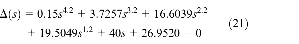
\begin{matrix} Δ (s) = 0.15 s^{4.2} + 3.7257 s^{3.2} + 16.6039 s^{2.2} \\ + 19.5049 s^{1.2} + 40 s + 26.9520 = 0 \end{matrix}

(21)

For α = 0.2, Equation (22) is obtained by writing w instead of $s^{α}$

\begin{matrix} Δ (w) = 0.15 w^{21} + 3.7257 w^{16} + 16.6039 w^{11} \\ + 19.5049 w^{6} + 40 w^{5} + 26.9520 = 0 \end{matrix}

(22)

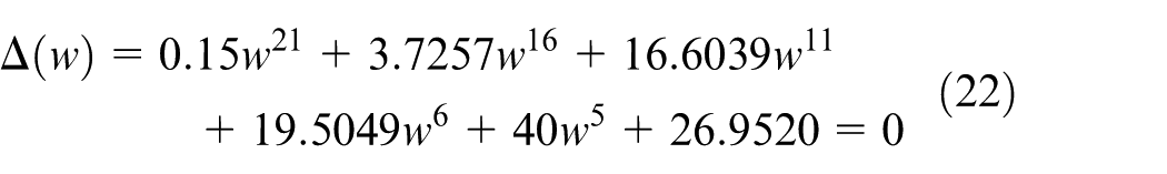
Equation (22) is solved using MATLAB software and roots are obtained as follows

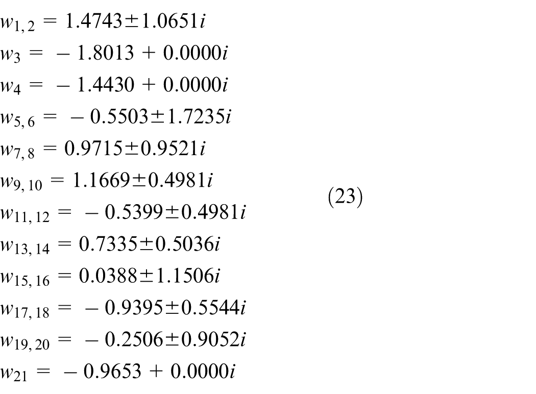
\begin{matrix} w_{1, 2} = 1.4743 \pm 1.0651 i \\ w_{3} = - 1.8013 + 0.0000 i \\ w_{4} = - 1.4430 + 0.0000 i \\ w_{5, 6} = - 0.5503 \pm 1.7235 i \\ w_{7, 8} = 0.9715 \pm 0.9521 i \\ w_{9, 10} = 1.1669 \pm 0.4981 i \\ w_{11, 12} = - 0.5399 \pm 0.4981 i \\ w_{13, 14} = 0.7335 \pm 0.5036 i \\ w_{15, 16} = 0.0388 \pm 1.1506 i \\ w_{17, 18} = - 0.9395 \pm 0.5544 i \\ w_{19, 20} = - 0.2506 \pm 0.9052 i \\ w_{21} = - 0.9653 + 0.0000 i \end{matrix}

(23)

The results obtained for this example are given in Figure 7. In the figure, stability analysis for controllers designed with the integral absolute error (IAE) criteria is presented. In the figure, the unstable region has an angle of 2 × 18 = 36°. It is seen that all of the roots obtained are in the stable region.

Figure 7.

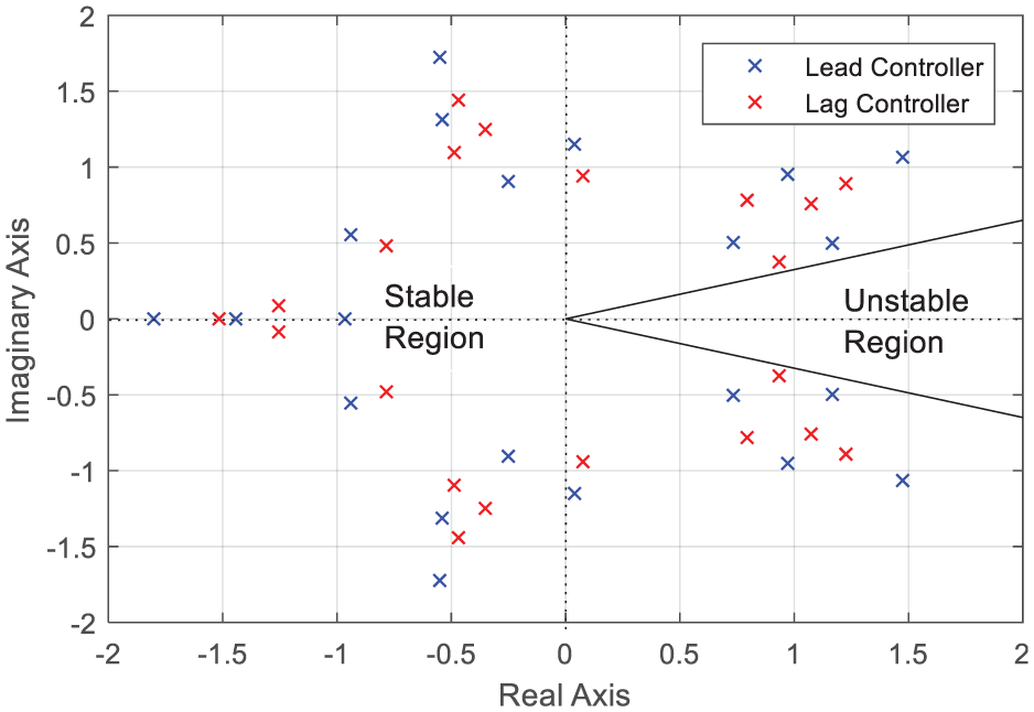
Poles position in complex w plane for Example 1.

Example 2

Consider the system with the transfer function given in Equation (24)

G_{p 2} (s) = \frac{1}{s^{1.5} (0.6 s + 1)}

(24)

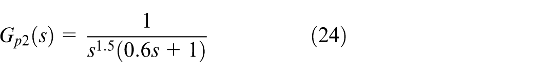
In this example, only the lead controller design was implemented, unlike the first example. Closed-loop unit-step response of the system with C(s) = 1 is shown in Figure 8.

Figure 8.

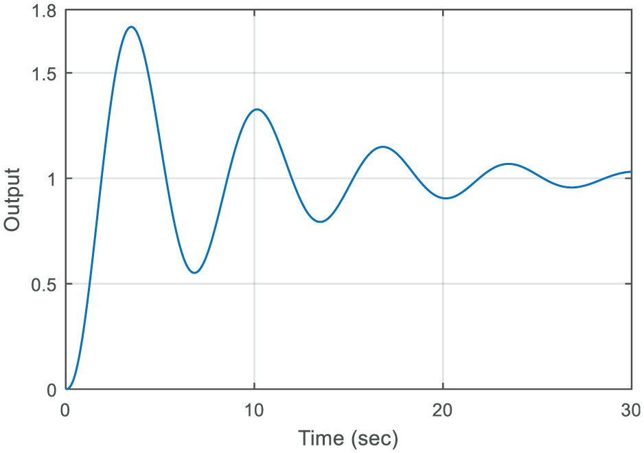
Step response of the closed loop system C(s) = 1 and G_p₂(s).

Optimization process is started by set down initial values in Simulink block diagram. The phase-lead controller parameters are found by stopping the optimization when the error reaches its minimum value. The determined phase-lead controller parameters are shown in Table 4. The controller parameters given in Table 4 are applied to Equation (1) and the lead controllers are obtained. By applying the controllers to the system given in Equation (24), Figure 9 is obtained.

Table 4.

The lead controller parameters and time domain performance values for Example 2.

	IAE	ISE	ITSE	ITAE
K	18.24	19.58	19.59	17.52
z	0.296	0.191	0.24	0.289
p	7.692	5.497	6.621	8.283
Rise time	0.64	0.46	0.53	0.73
Settling time	9.83	2.64	2.66	11.60
Peak time	1.34	1.04	1.14	1.51
Overshoot (%)	5.66	17.42	10.75	2.43

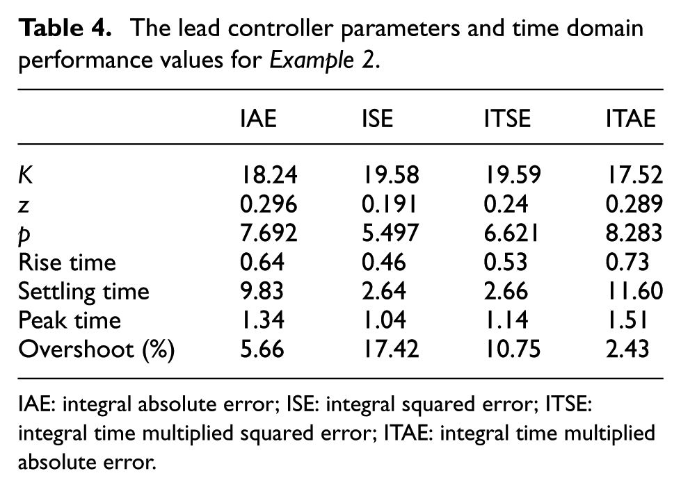
IAE: integral absolute error; ISE: integral squared error; ITSE: integral time multiplied squared error; ITAE: integral time multiplied absolute error.

Figure 9.

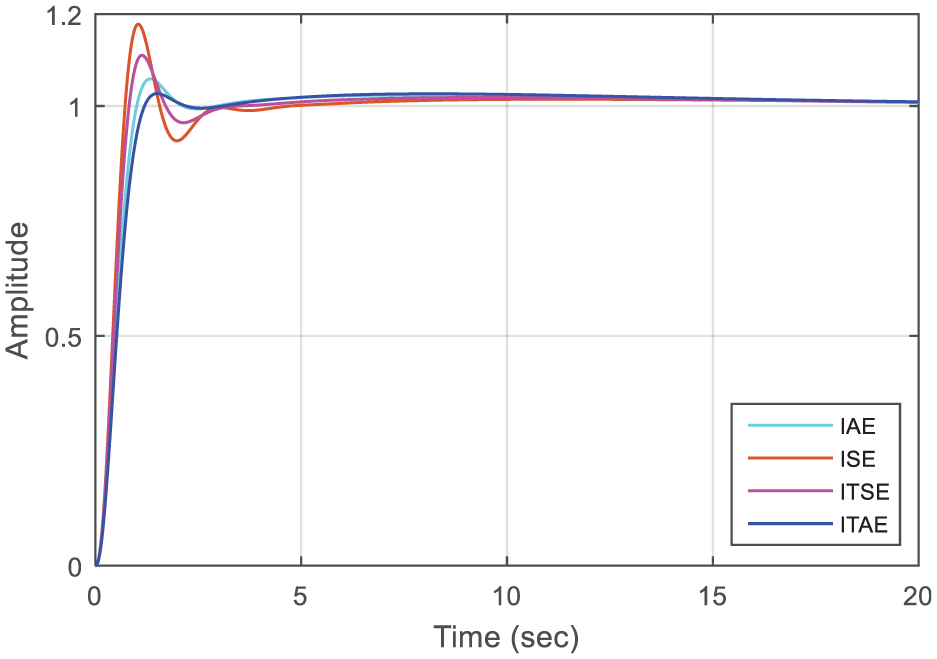
Step responses for G_p₂(s) with phase-lead controllers.

Although the percent overshoot of the system with C(s) = 1 was 71%, it decreases to 2.43% when controlled by the phase-lead controller. The lowest value in percent overshoot was obtained with the ITAE criterion. Also, Table 4 can be examined for details of performance characteristic. The settling time of the system with lead controller is realized in 2.64 s with the ISE criterion. It is noteworthy that with the ITAE criterion, where the lowest percent overshoot is achieved, the longest settling time is realized. The selection of the appropriate performance criterion for obtaining the desired time response is too important.

The stability analysis for systems with controller is given in Figure 10. In the figure, stability analysis was performed for four different systems. In the figure, the unstable region has an angle of 2 × 45 = 90°. It is seen that all of the roots obtained are in the stable region.

Figure 10.

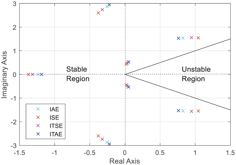
Poles position in complex w plane for Example 2.

There is no special method in the literature to design lag or lead controllers for the control systems with the fractional-order plant. For comparison, we use the frequency domain design method given by Ogata and Yang⁶ and the following controller for the system given in Equation (24) is designed

C (s) = \frac{1.663 (s + 0.509)}{(s + 1.818)}

(25)

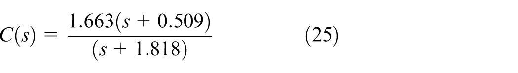
The unit-step responses of the controller obtained by the ITAE criterion and the Ogata’s method are given below. The performance of the controller obtained by optimization method is superior (Figure 11).

Figure 11.

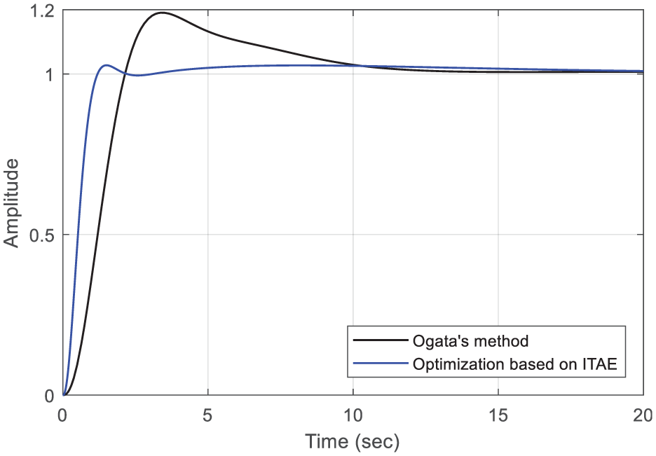
Step responses of the controllers using optimization method and Ogata method.

Example 3

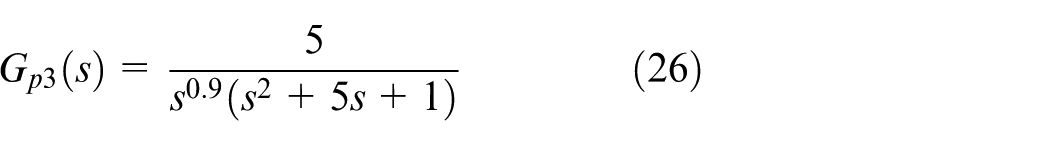
Consider a plant with the transfer function described in Equation (26)

G_{p 3} (s) = \frac{5}{s^{0.9} (s^{2} + 5 s + 1)}

(26)

Closed-loop unit-step response of the system with C(s) = 1 is shown in Figure 12. It is observed from Figure 12 that the unit-step response has a large overshoot and long settling time.

Figure 12.

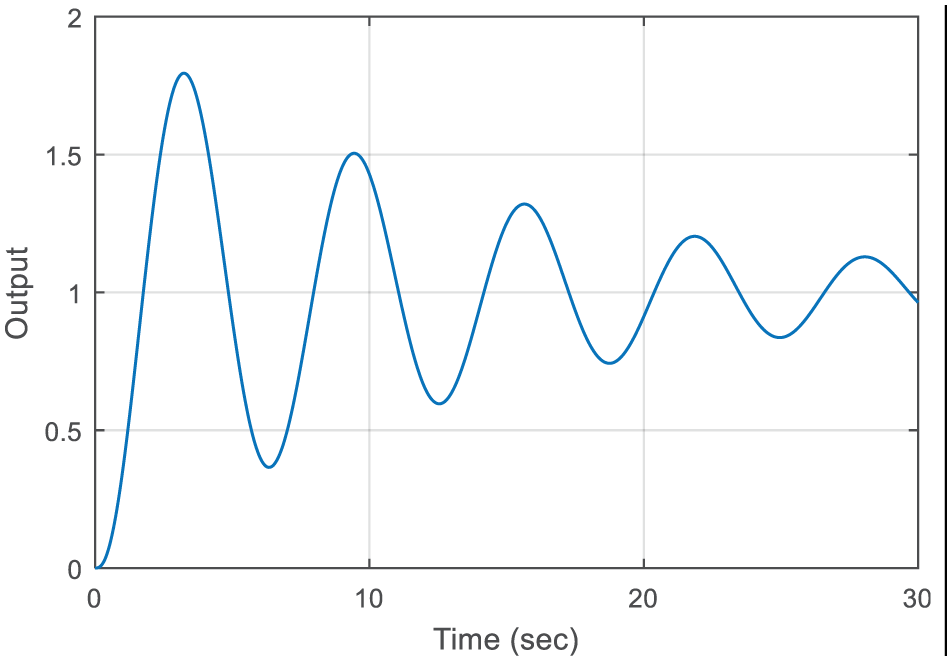
Step response of the closed loop system with C(s) = 1 and G_p₃(s).

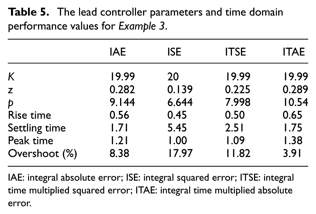
By applying the presented method to the system to be controlled, the controller parameters are obtained as in Table 5.

Table 5.

The lead controller parameters and time domain performance values for Example 3.

	IAE	ISE	ITSE	ITAE
K	19.99	20	19.99	19.99
z	0.282	0.139	0.225	0.289
p	9.144	6.644	7.998	10.54
Rise time	0.56	0.45	0.50	0.65
Settling time	1.71	5.45	2.51	1.75
Peak time	1.21	1.00	1.09	1.38
Overshoot (%)	8.38	17.97	11.82	3.91

IAE: integral absolute error; ISE: integral squared error; ITSE: integral time multiplied squared error; ITAE: integral time multiplied absolute error.

The controller parameters shown in Table 5 are applied to Equation (1) and the lead controllers are determined. By applying the controllers to the system given in Equation (26), Figure 13 is obtained.

Figure 13.

Step responses for G_p₃(s) with phase-lead controllers.

As seen from Figure 13, the percent overshoot values of closed loop systems with phase-lead controller decreases to about 3.91% using ITAE criterion. The IAE criterion provides the lowest settling time. Also the ISE criterion provides the fastest rise and settling time. Table 5 can be examined for details of performance characteristics. The percent overshoot in the system with lead controller drops to 3.91%, while the percent overshoot of the system without controller is about 79%. Similarly, while the settling time of the system without controller is approximately 53 s, the settling time in the system with lead controller decreases to 1.71 s. From these results, it is seen that the system is quickly and successfully controlled.

The stability analysis for systems with controller is given in Figure 14. In the figure, stability analysis was performed for four different systems. In the figure, the unstable region has an angle of 2 × 9 = 18°. It is seen that all of the roots obtained are in the stable region.

Figure 14.

Poles position in complex w plane for Example 3.

Example 4

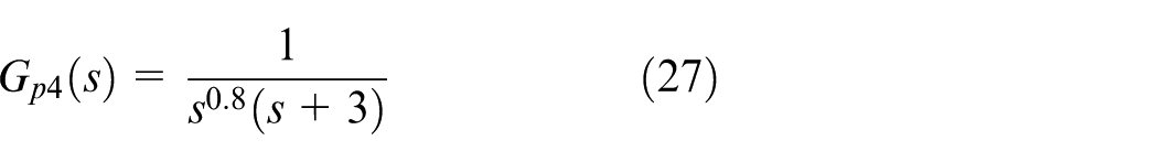
Consider a plant with the transfer function described in Equation (27)

G_{p 4} (s) = \frac{1}{s^{0.8} (s + 3)}

(27)

Closed-loop unit-step response of the system with C(s) = 1 is shown in Figure 15.

Figure 15.

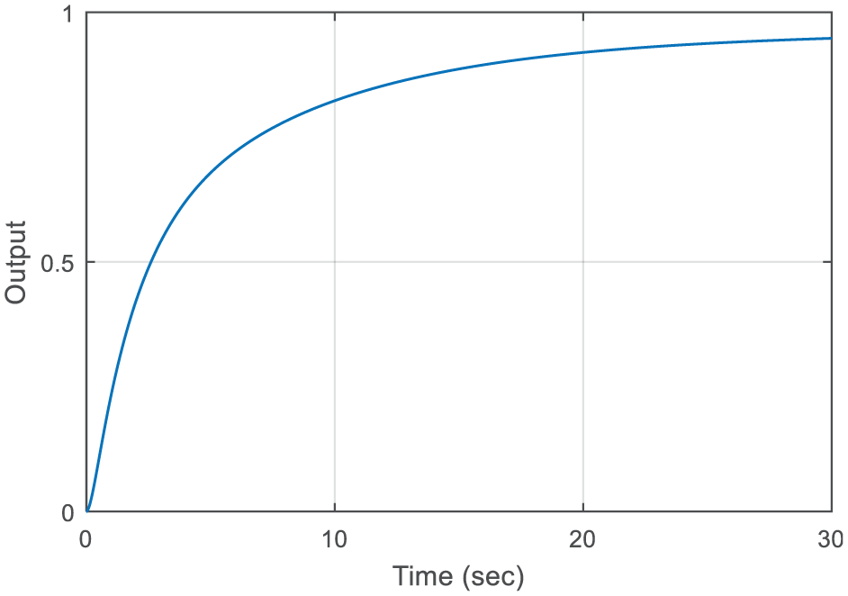
Step response of the closed loop system with C(s) = 1 and G_p₄(s).

By applying the method to the system to be controlled, the controller parameters are obtained as in Table 6. For this example, while lead controller was obtained with ITSE criterion, lag controllers were obtained with other criteria. The step responses obtained by applying the controllers to the system are presented in Figure 16.

Table 6.

The lead and lag controller parameters and time domain performance values for Example 4.

	IAE	ISE	ITSE	ITAE
K	17.824	20	20	18.785
z	15.972	20	3.42	14.058
p	12.549	15.746	4.167	11.383
Rise time	0.25	0.23	0.30	0.25
Settling time	1.44	1.33	1.54	1.41
Peak time	0.55	0.53	0.62	0.55
Overshoot (%)	22.80	24.95	9.93	23.31

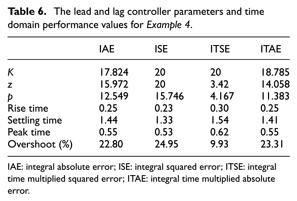
IAE: integral absolute error; ISE: integral squared error; ITSE: integral time multiplied squared error; ITAE: integral time multiplied absolute error.

Figure 16.

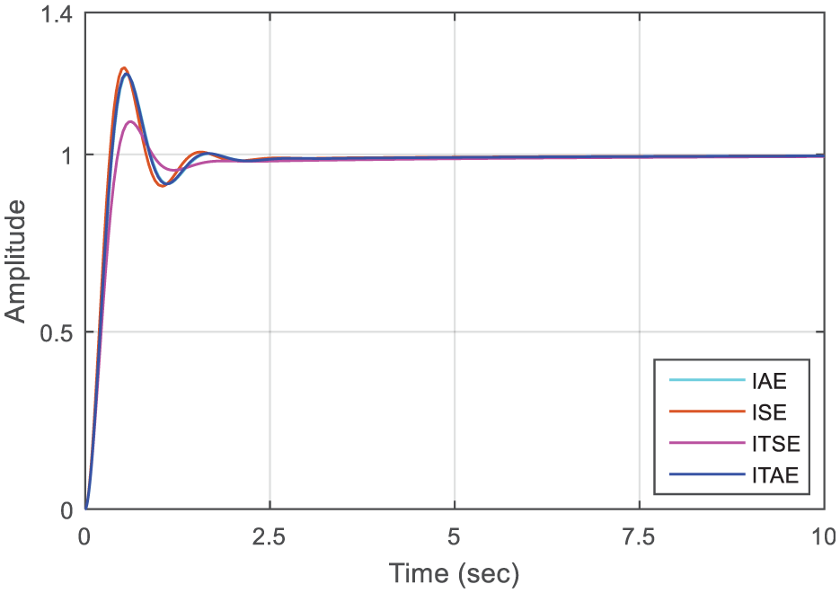
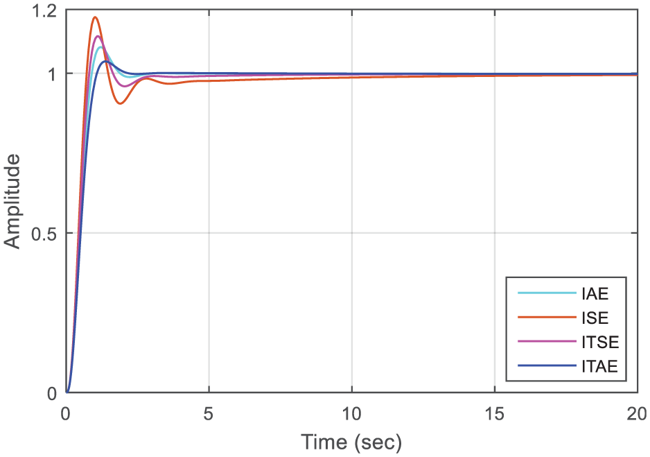
Step responses for G_p₄(s) with phase-lead and lag controllers.

As seen from Figure 16, the settling times provided using all the integral performance criteria are around 1.4 s. The lowest percent overshoot is provided by ITSE criterion about 9.93%. Table 6 can be examined for details of performance characteristic. For this example, the settling time is shortened to 1.33 s with the controller, while the settling time is at 104 s. It is seen that the fractional-order control systems have controlled by using a successful optimization method.

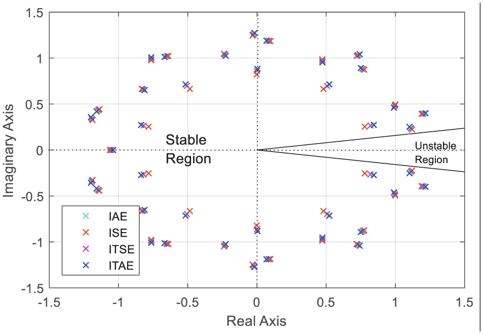
The stability analysis for systems with controller is given in Figure 17. In the figure, the unstable region has an angle of 2 × 18 = 36°.

Figure 17.

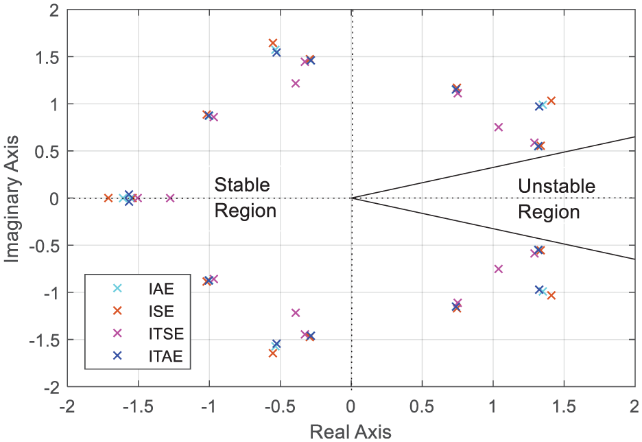
Poles position in complex w plane for Example 4.

Conclusion

In this study, lead and lag controllers design were carried out for the fractional-order systems using the optimization method. The basic concept here is to optimize the controller parameters to meet a performance criterion. The controller design was performed for each integral performance criterion. The transient response behavior of a system plays an important role in monitoring performance. Therefore, integral performance criteria such as ISE, IAE, ITSE and ITAE are commonly used in control systems.

When designing a phase-lead controller, the ITAE performance criterion provides lowest percent overshoot value for the given examples, outside of the Example 4. The ISE performance criterion, however, causes the largest percent overshoot. In Example 1, when designing a phase-lag controller, the lowest percent overshoot value is obtained using by ITAE performance criterion. However, the ISE performance criterion causes the largest percent overshoot as in the design of the phase-lag controller. In the design of a controller, the choice of the integral performance criterion can be decided according to the nature of the system to be designed.

In the presented study, a phase-lead and phase-lag controller design has been done successfully for fractional-order systems.

Footnotes

Appendix 1

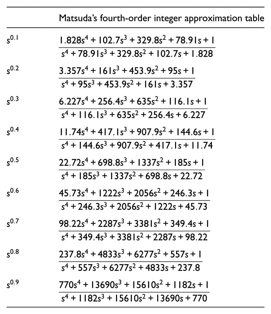
	Matsuda’s fourth-order integer approximation table
$s^{0.1}$	$\frac{1.828 s^{4} + 102.7 s^{3} + 329.8 s^{2} + 78.91 s + 1}{s^{4} + 78.91 s^{3} + 329.8 s^{2} + 102.7 s + 1.828}$
$s^{0.2}$	$\frac{3.357 s^{4} + 161 s^{3} + 453.9 s^{2} + 95 s + 1}{s^{4} + 95 s^{3} + 453.9 s^{2} + 161 s + 3.357}$
$s^{0.3}$	$\frac{6.227 s^{4} + 256.4 s^{3} + 635 s^{2} + 116.1 s + 1}{s^{4} + 116.1 s^{3} + 635 s^{2} + 256.4 s + 6.227}$
$s^{0.4}$	$\frac{11.74 s^{4} + 417.1 s^{3} + 907.9 s^{2} + 144.6 s + 1}{s^{4} + 144.6 s^{3} + 907.9 s^{2} + 417.1 s + 11.74}$
$s^{0.5}$	$\frac{22.72 s^{4} + 698.8 s^{3} + 1337 s^{2} + 185 s + 1}{s^{4} + 185 s^{3} + 1337 s^{2} + 698.8 s + 22.72}$
$s^{0.6}$	$\frac{45.73 s^{4} + 1222 s^{3} + 2056 s^{2} + 246.3 s + 1}{s^{4} + 246.3 s^{3} + 2056 s^{2} + 1222 s + 45.73}$
$s^{0.7}$	$\frac{98.22 s^{4} + 2287 s^{3} + 3381 s^{2} + 349.4 s + 1}{s^{4} + 349.4 s^{3} + 3381 s^{2} + 2287 s + 98.22}$
$s^{0.8}$	$\frac{237.8 s^{4} + 4833 s^{3} + 6277 s^{2} + 557 s + 1}{s^{4} + 557 s^{3} + 6277 s^{2} + 4833 s + 237.8}$
$s^{0.9}$	$\frac{770 s^{4} + 13690 s^{3} + 15610 s^{2} + 1182 s + 1}{s^{4} + 1182 s^{3} + 15610 s^{2} + 13690 s + 770}$

Declaration of conflicting interests

The author(s) declared no potential conflicts of interest with respect to the research, authorship, and/or publication of this article.

Funding

The author(s) disclosed receipt of the following financial support for the research, authorship, and/or publication of this article: This work is supported by the Scientific and Research Council of Turkey (TÜBİTAK) under Grant no. EEEAG-115E388.

ORCID iD

Tufan Dogruer

References

Åström

Hägglund

PID controllers: theory, design, and tuning. Triangle Park, NC: Instrument Society of America Research, 1995.

Barbosa

Machado

Ferreira

IM.

Tuning of PID controllers based on Bode’s ideal transfer function. Nonlinear Dynam 2004; 38: 305–321.

Monje

Vinagre

Feliu

, et al. Tuning and auto-tuning of fractional order controllers for industry applications. Control Eng Pract 2008; 16: 798–812.

Petras

The fractional-order controllers: Methods for their synthesis and application, 2000, https://arxiv.org/abs/math/0004064

Tan

Computation of stabilizing PI and PID controllers for processes with time delay. ISA T 2005; 44: 213–223.

Ogata

Yang

Modern control engineering. New Delhi, India: Prentice Hall, 2002.

Loh

Cai

Tan

WW.

Auto-tuning of phase lead/lag compensators. Automatica 2004; 40: 423–429.

Yeung

Lee

KH.

A universal design chart for linear time-invariant continuous-time and discrete-time compensators. IEEE T Educ 2000; 43: 309–315.

Murray

RM.

Optimization-based control. Pasadena, CA: California Institute of Technology, 2009.

10.

Horng

Lead-lag compensator design based on genetic algorithms. In: Proceedings of the conference on technologies and applications of artificial intelligence, Tainan, 16–18 November 2012, pp. 80–85. New York: IEEE.

11.

Monje

Vinagre

Calderón

, et al. Auto-tuning of fractional lead-lag compensators. IFAC P Vol 2005; 38: 319–324.

12.

Yeroglu

Tan

Classical controller design techniques for fractional order case. ISA T 2011; 50: 461–472.

13.

Salehtavazoei

Tavakoli-Kakhki

Compensation by fractional-order phase-lead/lag compensators. IET Control Theory A 2014; 8: 319–329.

14.

Khiabani

Babazadeh

Design of robust fractional-order lead–lag controller for uncertain systems. IET Control Theory A 2016; 10: 2447–2455.

15.

Atherton

Control engineering. London: Bookboon, 2009.

16.

Faieghi

Nemati

On fractional-order PID design. In: Michalowski

(ed.) Applications of MATLAB in science and engineering. Rijeka: Intech, 2011.

17.

Matsuda

Fujii

H (infinity) optimized wave—absorbing control—analytical and experimental results. J Guid Control Dynam 1993; 16: 1146–1153.

18.

Oustaloup

Levron

Mathieu

, et al. Frequency-band complex noninteger differentiator: characterization and synthesis. IEEE T Circuits-I 2000; 47: 25–39.

19.

Carlson

Halijak

Approximation of fractional capacitors (1/s)(1/n) by a regular Newton process. IEEE T Circuit Theory 1964; 11: 210–213.

20.

Yin

Zhong

S-m

Huang

, et al. Robust stability analysis of fractional-order uncertain singular nonlinear system with external disturbance. Appl Math Comput 2015; 269: 351–362.

21.

Luo

Chen

Wang

, et al. Tuning fractional order proportional integral controllers for fractional order systems. J Process Contr 2010; 20: 823–831.

22.

Hamamci

SE.

An algorithm for stabilization of fractional-order time delay systems using fractional-order PID controllers. IEEE T Automat Contr 2007; 52: 1964–1969.

23.

Yin

Huang

Chen

, et al. Fractional-order exponential switching technique to enhance sliding mode control. Appl Math Model 2017; 44: 705–726.

24.

Zhao

Xue

Chen

A fractional order PID tuning algorithm for a class of fractional order plants. In: Proceedings of the IEEE international conference mechatronics and automation, Niagara Falls, ON, 29 July–1 August 2005, pp. 216–221. New York: IEEE.

25.

Monje

Chen

Vinagre

, et al. Fractional-order systems and controls: fundamentals and applications. London: Springer Science & Business Media, 2010.

26.

Matušů

Application of fractional order calculus to control theory. Int J Math Model Methods Appl Sci 2011; 5: 1162–1169.

27.

Tustin

Allanson

Layton

, et al. The design of systems for automatic control of the position of massive objects. P I Electr Eng-C 1958; 105: 1–57.

28.

Manabe

The noninteger integral and its application to control systems. Engl Transl J Japan 1961; 6: 83–87.

29.

Manabe

The system design by the use of a model consisting of a saturation and noninteger integral.

Engl Transl J Japan 1963: 47–150.

30.

Miller

Ross

An introduction to the fractional calculus and fractional differential equations. New York: Wiley, 1993.

31.

Podlubny

Fractional-order systems and PIλDµ controllers. IEEE T Automat Contr 1999; 44: 208–214.

32.

Chen

Petras

Xue

Fractional order control-a tutorial. In: Proceedings of the American control conference, ACC’09, St. Louis, MO, 10–12 June 2009, pp. 1397–1411. New York: IEEE.

33.

Choudhary

SK.

Stability and performance analysis of fractional order control systems. WSEAS T Syst Contr 2014; 9: 438–444.

34.

Sabatier

Moze

Farges

LMI stability conditions for fractional order systems. Comput Math Appl 2010; 59: 1594–1609.

35.

Senol

Yeroglu

Tan

Analysis of fractional order polynomials using Hermite-Biehler theorem. In: Proceedings of the International conference on fractional differentiation and its applications ICFDA’14, Catania, 23–25 June 2014, pp. 1–5. New York: IEEE.

36.

Tavazoei

Haeri

A note on the stability of fractional order systems. Math Comput Simulat 2009; 79: 1566–1576.

37.

Matignon

Stability results for fractional differential equations with applications to control processing. Comput Eng Syst Appl 1996; 2: 963–968.

38.

Matignon

Stability properties for generalized fractional differential systems. ESAIM: Proc 1998; 5: 145–158.

39.

Matignon

Generalized fractional differential and difference equations: stability properties and modelling issues. In: Proceedings of the mathematical theory of networks and systems symposium, IL Poligrafo, Padova, July 1998, pp. 503–506.

40.

Pan

Das

Intelligent fractional order systems and control: an introduction. Berlin: Springer, 2012.

41.

Petráš

Stability of fractional-order systems with rational orders, 2008, https://arxiv.org/pdf/0811.4102.pdf

42.

Tavazoei

MS.

Notes on integral performance indices in fractional-order control systems. J Process Contr 2010; 20: 285–291.

43.

MathWorks (ed.). Optimization toolbox user’s guide R2018b, 2018, https://www.mathworks.com/help/pdf_doc/optim/optim_tb.pdf

Lead and lag controller design in fractional-order control systems

Abstract

Keywords

Introduction

Fundamentals of fractional-order systems and stability analysis

Integral performance criteria and optimization method

Implementation of the optimization method

Example 1

Example 2

Example 3

Example 4

Conclusion

Footnotes

Appendix 1

Declaration of conflicting interests

Funding

ORCID iD

References