Sage Journals: Discover world-class research

Abstract

The accuracy of computer numerical control machine tools can be improved by identifying error sources affecting the overall position error and orientation errors. Because of their inevitable nature, the position errors cannot be entirely eliminated from the machinery, but they can be identified, measured and compensated during the manufacturing process of the components by developing and using a mathematical model. In this present work, different mathematical models have been developed for the errors measured by laser interferometer at different nominal positions of X, Y and Z axes both in forward and reverse direction movement as per VDI 3441 Germany standard. Using Akaike information criterion, the best model is selected for each axis and later the best model’s coefficients have been optimized by considering both minimizing sum square errors and maximizing R² values using teaching–learning-based optimization algorithm. Technique for Order Preference by Similarity to the Ideal Solution method has been adopted to convert the dual objectives into a single objective. An improvement of 1%–71% in R² values was reported to prove the effectiveness of the proposed optimization algorithm, Teaching–Learning-Based Optimization algorithm, with the same sum square error values.

Keywords

Position errors mathematical model optimization TOPSIS method TLBO algorithm AIC method

Introduction

Globalization causes international competition among the manufacturers in selling their quality product with competitive prices. The components of a quality product are manufactured from quality machines. The position errors play a vital role in defining the cost and quality of a precision machine. Uncontrolled errors present in machines are the main reason in producing components with under or oversized condition which is not accepted by the customer because of their unacceptable dimension. Sometimes, this error causes secondary operation or rework to make it a customer-desired component.

Vinod et al.¹ developed a module to measure and compensate the position error of an axis using an open architecture motion controller and backpropagation feed forward neural network. This paper highlights the various sources of error like geometric error, cutting force induced error and thermal errors.² Ball bar test has been done on Vertical Machining Center (VMC) to find the circularity error of spindle, and vibration has been monitored.³ Liu et al.⁴ measured positioning error and backlash error by VM101 Linear encored measurement system by compensating backlash error. Quality and productivity of VMC have been greatly improved by accuracy assessment of machine tools and condition monitoring.⁵ Neural network system was developed to perform positioning error compensation in the lathe by laser interferometer.⁶ Laser autocollimator had been used to measure angular error, and the neural network has been used to predict error and compensation.⁷ By incorporating four steps of measurement of error components by using a laser interferometer system, artificial neural network (ANN) has been used for online error measurement using sensors. Synthesis of total error into three-dimensional (3D) error kinematic model of error compensation is the ultimate step.⁸ Disadvantages of using lookup table had been highlighted as it requires extensive memory. Neural network had resulted in lesser memory.⁹ A review of different instruments to measure machine tools had been discussed.¹⁰ Linear displacement accuracy showed improvement for computer numerical control (CNC) machine by applying positive and negative direction pitch error compensation.¹¹ Linear displacement error of CNC Lathe, CNC milling center and deep drilling machine had been measured. Renishaw laser measurement system showed a better result.¹² After measuring the linear error by laser interferometer, linear error compensation package had been measured and fed into the machine controller to enhance the machine accuracy.¹³ Geometric error components had been measured using QC 20 Ball and Genetic Algorithm-Particle Swarm Optimization (GA-PSO) had been incorporated to find optimal error values.¹⁴ By the compensation of volumetric error and on-machine measurement using a touch trigger probe, the accuracy of the machine tool has been increased.¹⁵Magnetic ball bars and the telescopic version were utilized to measure machine errors.¹⁶ Straightness error was measured by two laser systems, Renishaw and Damalini laser measurement system. Renishaw laser measuring system was more flexible and more precise, and accurate readings were obtained.¹⁷ Laser interferometer was used to detect and compensate machine screw pitch error compensation.¹⁸ A 3D probe ball combines the concept of well-known double bar ball (DBB) and three dimensions measuring probe, an extension bar and a base plate with a central ball on the upper side.^19,20 The predicted compensation method has been used to calculate the correction vector in machine coordinates from the predicted tool pose error in workpiece coordinates. Rotary axis errors constitute dominant 80% and linear axes comprise 20% error. Overall positioning errors had been measured by 3D probe ball.^21,22 Telescoping magnetic DBB had been used to measure the motion and link errors of machine tools by performing circular tests.²³ Wang et al.^24–26 have focused on non-contact laser technique and laser vector measurement methods in compensating errors by finding error budget. Translational axes are kept stationary and two rotary axes are focused to move and obtain a circular trajectory. Finally, eight position independent geometric errors (PIGES) had provided better accurate results.^27–29 The geometric error has been measured and compensated.³⁰ Using laser tracker, real-time corrections of the machine tool absolute volumetric error has been achieved.³¹ Modeling, prediction and compensation of thermal errors have been dealt.^32–34

Problem definition

Performance or function of the product depends on the quality or dimensional accuracy of the sub-assemblies made up of precise components. The cost of machines which produce the accurate dimension of the components increases the prize of the product due to the manufacturing of the acceptable component’s dimension to meet out the quality and life of the product. This would satisfy the customer’s need. Position error plays an important role in precision machinery which controls the cost of the component produced by them. Errors which are not compensated present in the machines play a vital role in deciding the value of position errors. Unaccepted component due to their over or undersized dimension is obtained as a result of position errors which exist in the quality/high precise machines. This position error increases the manufacturing cost of the precise component and, in turn, causes the hike in the product cost.

Methodology

In this present work, the proposed work has been solved in four stages. In the first stage, the position errors have been measured using laser interferometer with equal interval movement of the axes X, Y and Z both in forward and reverse direction. Different mathematical models have been developed to calculate the position error with the measured data in the second stage. Using the Akaike information criterion (AIC), the best model has been selected in the third stage. In the final stage, the coefficients of the best model have been optimized by considering dual objectives of minimizing sum square error (SSE) and maximizing R² values using teaching–learning-based optimization (TLBO) algorithm where Technique for Order Preference by Similarity to the Ideal Solution (TOPSIS) method has been adopted to convert the dual objectives into single objective. Third and fourth stages are the novelty of the present work. The novelty of the article differs in two ways with the existing work. The first one is developing different mathematical models and comparing the models based on the number of terms involved in calculating the measured error by using AIC. In the second one, the coefficients of the selected models are optimized using TLBO algorithm with the dual objectives of minimizing the SSE and maximizing the R² values by adopting the TOPSIS method.

Measurement of error in nominal position of axes

The working volume of the machining center considered in this work is 710 × 500 × 500 mm. VMC has to run for 2–3 h before measuring positioning errors to avoid thermal error. At a feed rate of 50 mm/min, a warm-up cycle for VMC is to be carried out in both forward and reverse direction. This was conducted to reduce thermal-related error. Measurement standards expect the machine to undergo thermal transition state before attaining steady-state equilibrium. According to VDI 3441Germany standard, each run includes one forward stroke and one reverse stroke. For each axis, five measurements were taken and linear positioning data were taken, and linear positioning data were measured at equal intervals of every 20 mm.

Development of mathematical model

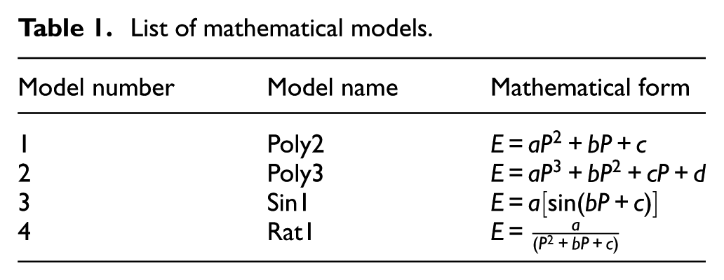
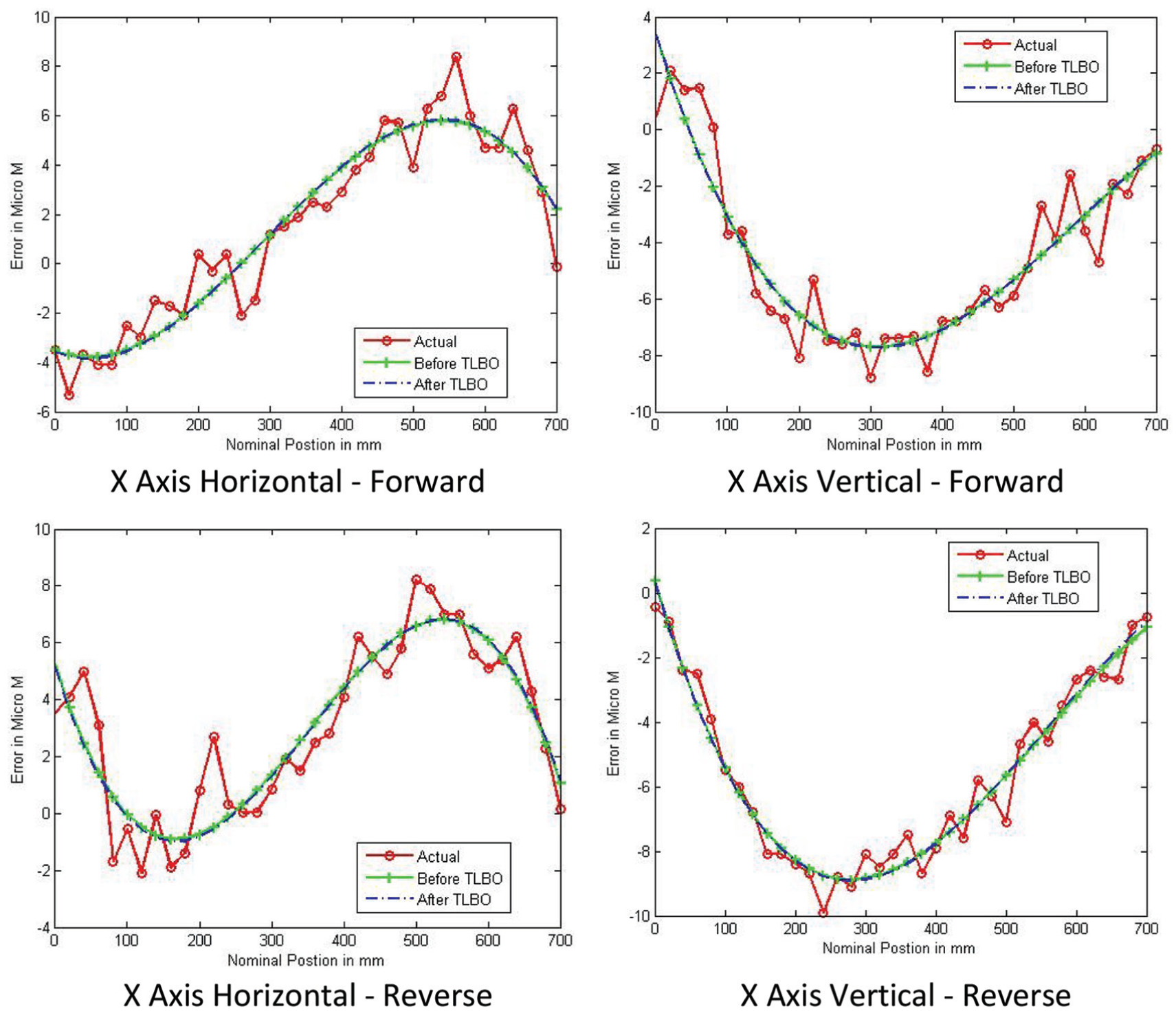
Figure 1 represents the error measured both in the horizontal and vertical direction of X, Y and Z axes with forward and reverse motion. Using the nominal position and error values of each axis, four different models like “Poly2,”“Poly3,”“Sin1” and “Rat1” have been developed using MATLAB function “fit,” and their mathematical model is given in Table 1. For demonstration, the mathematical model of “Poly3” is represented in Equation (1). The coefficients, SSE and R² values of each model for each axis of X, Y and Z, are presented in Tables 2

E = a P^{3} + b P^{2} + c P + d

(1)

where,

E—Calculated error in µm

a, b, c & d—Coefficients

P—Nominal position value in mm

Figure 1.

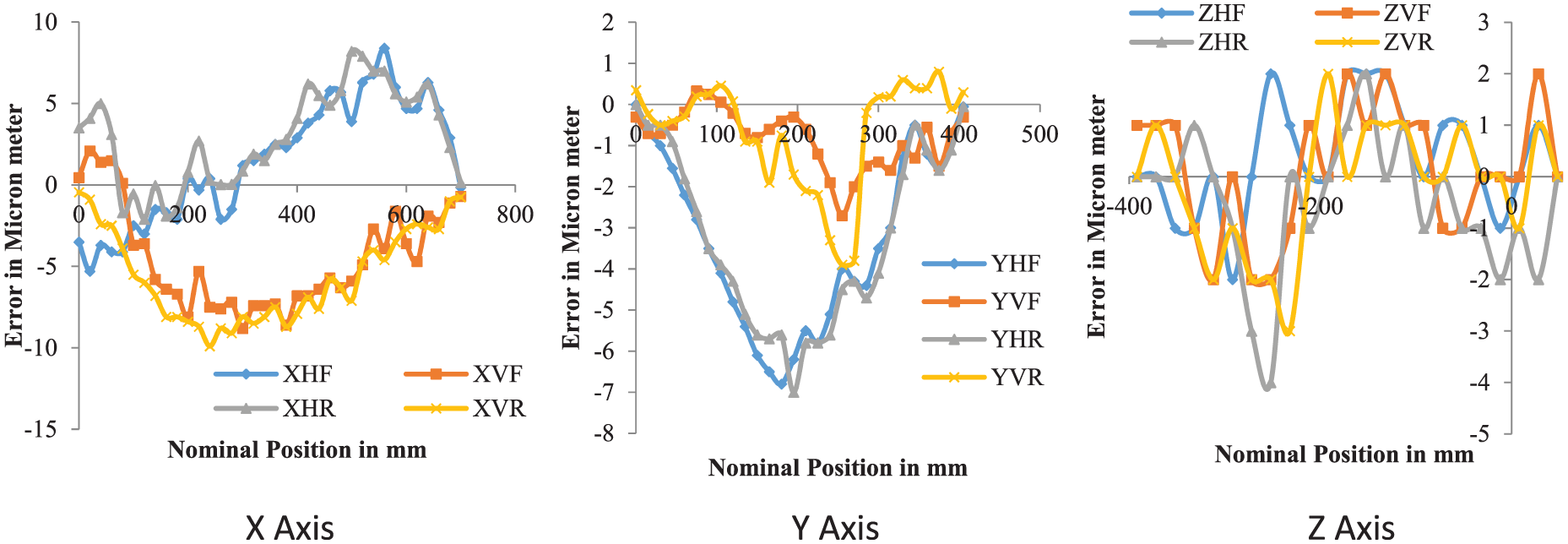
Measured error in X, Y and Z axes.

Table 1.

List of mathematical models.

Model number	Model name	Mathematical form
1	Poly2	$E = a P^{2} + b P + c$
2	Poly3	$E = a P^{3} + b P^{2} + c P + d$
3	Sin1	$E = a [\sin (b P + c)]$
4	Rat1	$E = \frac{a}{(P^{2} + b P + c)}$

Table 2.

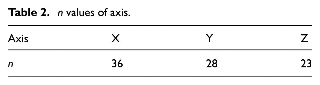
n values of axis.

Axis	X	Y	Z
n	36	28	23

Selection of the best mathematical model

It is necessary to select the best mathematical model from the given models in such a way that it shouldn’t be either overfitting or more complex in nature in determining the prediction value of error. AIC is used to solve this problem in a simple way. This is the first contribution of the authors in the present work. It consists of two terms, namely maximized likelihood term and number of free parameters used in the model. It is represented in Equation (2). Further reading about the information of AIC can be found in Akaike^35–41

A I C = - 2 L o g (L) + 2 K

(2)

where,

L—Maximized likelihood function,

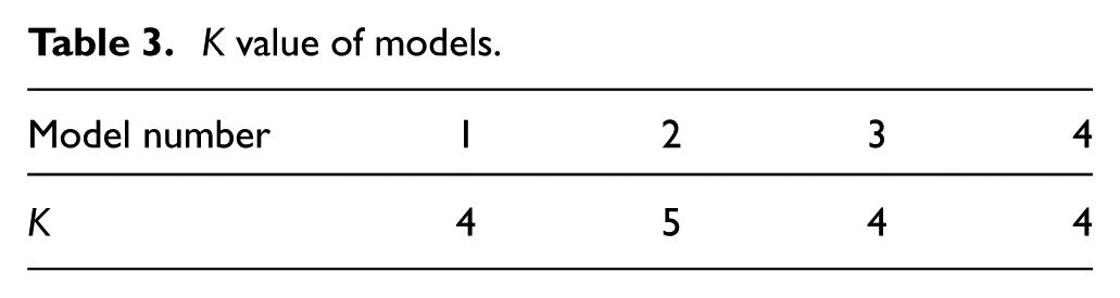
K—Number of coefficients in the model plus one.

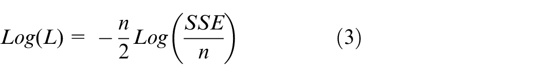
The value of Log (L) can be calculated using Equation (3) where “n” represents number of readings. The number of readings (n) in each axis and the number of coefficients (K) of each model are listed in Tables 2 and 3.

L o g (L) = - \frac{n}{2} L o g (\frac{S S E}{n})

(3)

Table 3.

K value of models.

Model number	1	2	3	4
K	4	5	4	4

The value of AIC of each model for each axis is determined using Equations (2) and (3) by substituting the values of SSE, n and K presented in Table 4. Figure 2 represents the value of AICs of different models for X, Y and Z axes.

Table 4.

Coefficients of mathematical models for X-axis.

Model number	Model name	Coefficients				SSE	R ²
Model number	Model name	a	b	c	d	SSE	R ²
1	XHF	–2.64267E–05	0.033812	–6.01859		90.8	0.81565
	2	–1.5943E–07	0.000141	–0.0124	–3.5143	45.8	0.90707
	3	5.110503631	0.005339	–1.32023		60.7	0.87669
	4	–13440.79461	–84.45466	4481.353		474.7	0.03637
1	XVF	7.19E–05	–0.051854	1.765162		62.2	0.81843
	2	–1.01E–07	0.000178	–0.08119	3.35477	44.0	0.87141
	3	7.802436304	0.004782	3.00212		62.4	0.81769
	4	0.092346322	–17.05398	0.189932		1063.6	–2.1058
1	XHR	2.19E–06	0.006129	0.466876		215.1	0.29842
	2	–3.05E–07	0.000322	–0.08217	5.2517	50.7	0.83474
	3	5.284175181	0.00198	–0.03917		213.2	0.30444
	4	32102.62024	71.96589	8096.799		568.1	–0.8534
1	XVR	6.65E–05	–0.043659	–1.31592		31.8	0.88685
	2	–1.07E–07	0.000179	–0.07459	0.3601	11.7	0.95856
	3	8.667466045	0.004289	–2.95984		28.5	0.89863
	4	–406.295136	–104.4247	516.0314		1372.1	–3.8778

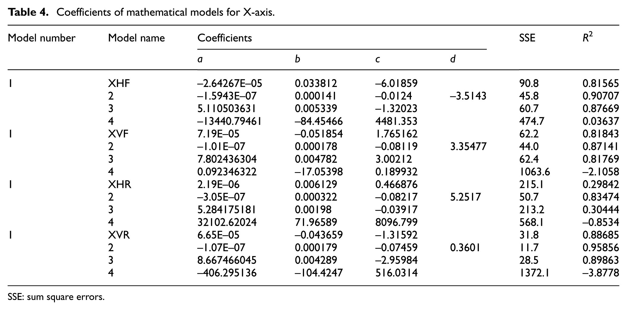
SSE: sum square errors.

Figure 2.

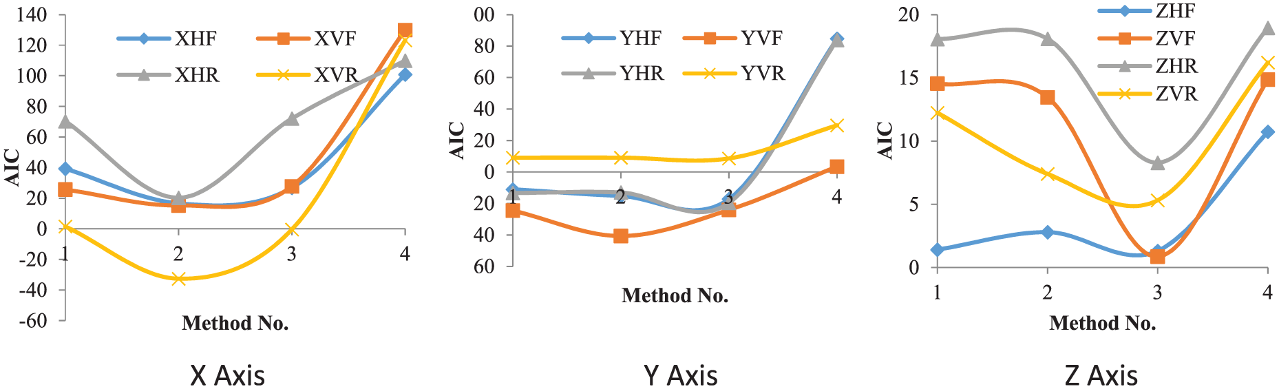
Value of AIC for different models.

Optimization of coefficients of the best model

In this section, the coefficients of the best model of each axis are optimized using TLBO algorithm, considering both minimizing SSE and maximizing R² values by adopting the TOPSIS method. This is the second contribution of the author in the present research work.

TLBO algorithm

Nature inspired evolutionary algorithms like GA, Ant Colony Optimization (ACO), PSO, Harmony Search (HS) and Artificial Bee Colony (ABC) are probabilistic algorithms which require a set of control parameters such as population size, number of generation and so on, and apart from that each algorithm also require specific control parameters. For example, PSO requires inertia weight, social and cognitive parameters, whereas in GA the mutation and crossover rate play a crucial role that affects the performance of the algorithms. The setting of these parameters affects the computational time and also end with local optimal solution. TLBO is a robust and effective method which doesn’t require any tuning of control parameters. Because of the above advantages of TLBO as compared to other optimization techniques, it is implemented in this work. This algorithm mimics the teaching–learning environment happening between the students and teacher in a classroom. In this process, the student performance can be improved by both the teacher and students themselves. The performance of the student is treated as objective function of the proposed work. Basic concepts of TLBO are found in Rao.⁴²,^43,45 Application of TLBO in various fields is found in Rao.^45,46,47,49.

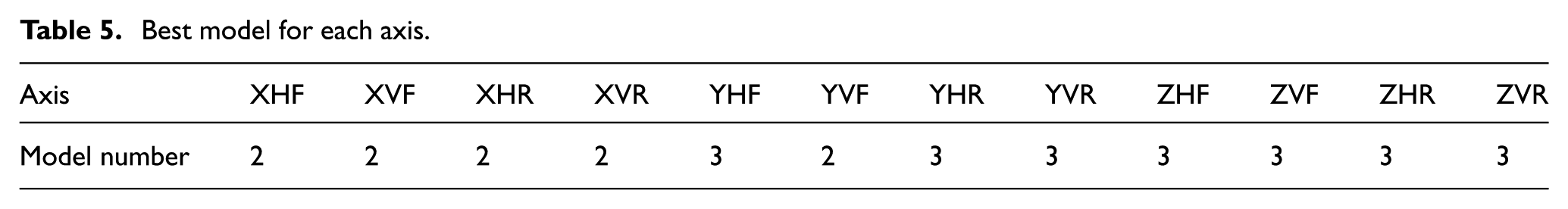
The model which has low AIC will be the best model, hence from the above Figure 2 the best model is selected for each axis for both directions and represented in Table 5.

Table 5.

Best model for each axis.

Axis	XHF	XVF	XHR	XVR	YHF	YVF	YHR	YVR	ZHF	ZVF	ZHR	ZVR
Model number	2	2	2	2	3	2	3	3	3	3	3	3

Conversion of dual objectives into single objective using TOPSIS method

The accuracy of conversion method from multiple objectives to single objective leads to produce the best-optimized values for the models. Usual methods like weighted sum, normalization, desirability function and so on sometimes leads to the non-optimal selection of process parameters. Hence, in this work TOPSIS method has been implemented to get correct optimized parameters. This method was initially presented by Hwang and Yoon and later on developed and implemented by many authors^50–52 in different fields. Renishaw touch trigger probe had been used for accuracy enhancement of coordinate measuring machine (CMM).⁵³ Pixel calibration was used in new machine vision-based tool position verification to measure real-time intricate dimensions.⁵⁴ Spindle residual vibration has been reduced by the sensorless balance method.⁵⁵ A. probe can determine the measurement accuracy of the CMM. A mathematical model had been developed between equivalent diameter and measuring force by simulated annealing.⁵⁶ EASY 5X simulation package had been used for modeling and optimization of CMM.⁵⁷ ANN had been used to reduce backlash error in VMC.⁵⁸

Implementation of TOPSIS method and TLBO algorithm

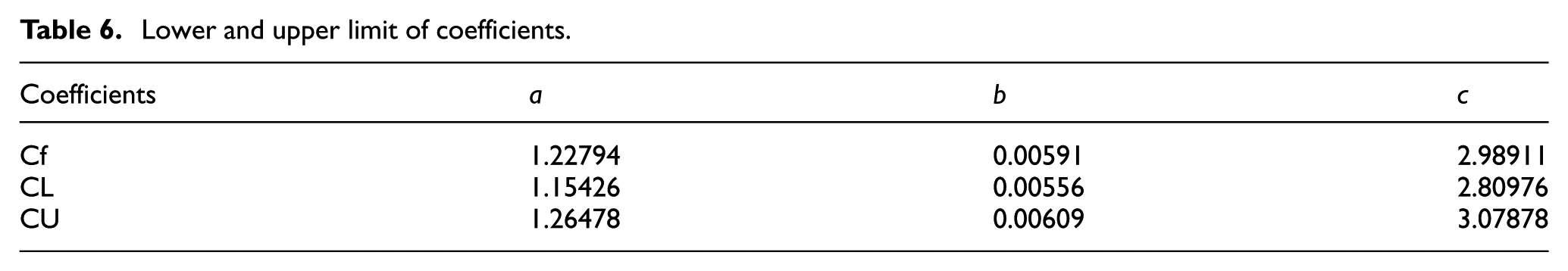
TLBO algorithm along with TOPSIS method has been implemented in this work to optimize the coefficients of different models selected for each axis in the previous section with the objective of minimizing SSE and maximizing R² values. It is shown in Figure 3.Table 6 represents the lower and upper bound values of the coefficients represented in the selected model. The step-by-step procedure of implementation is shown in Figure 3. For demonstration purpose, the proposed algorithm is implemented in optimizing the coefficients of the mathematical model number 2 for X-axis vertical direction reverse movement with the initial size of eight students.

Figure 3.

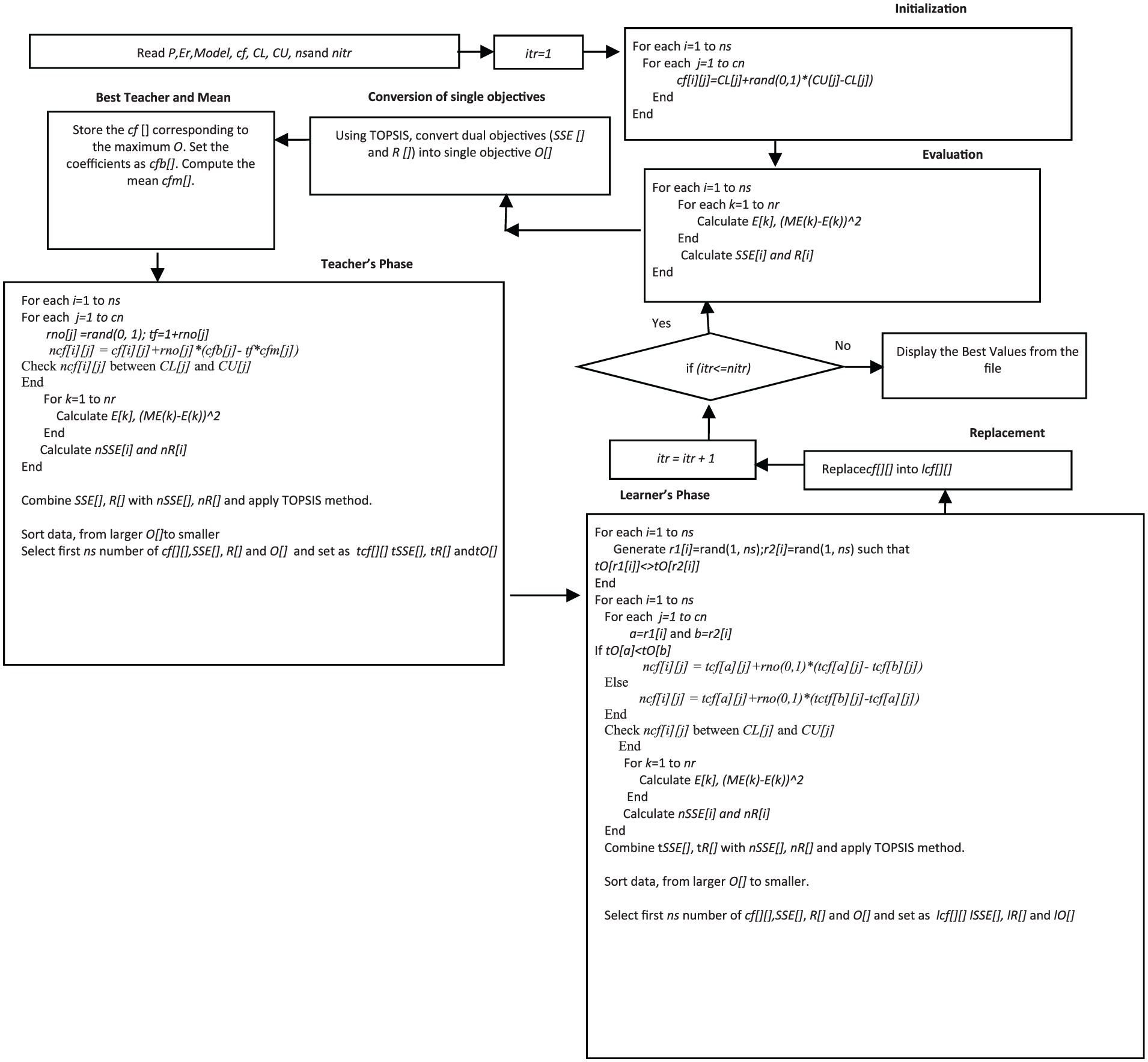
Implementation of TLBO algorithm.

Table 6.

Lower and upper limit of coefficients.

Coefficients	a	b	c
Cf	1.22794	0.00591	2.98911
CL	1.15426	0.00556	2.80976
CU	1.26478	0.00609	3.07878

Result and discussion

The optimized coefficients along with SSE and R² are given in Table 7 for all axes. It is understood in Table 7 that the optimized coefficients would be able to produce the improved R² values with the similar SSE value for all axes. The comparison of R² before and after the implementation of TLBO has been shown in Figure 4. It is observed that R² values obtained after the implementation of TLBO in all axes are higher than the values before implementation. Figure 5 shows the graph between the nominal position and measured error, calculated error obtained before and after the implementation of TLBO for all axes. The calculated errors obtained after the implementation of TLBO are closer with the measured error in almost all axes. Different mathematical models like polynomial second and third order, sine model and rational model have been developed and their results are compared based on AIC and the best model is selected for each axes both in forward and reverse direction.

Table 7.

Best coefficients, SSE and R² values for all axes.

Axis	Model Number	Coefficients				SSE	R ²
		a	b	c	d
XHF	2	–1.60817E–07	0.00014	–0.0123	–3.5807	45.8	0.92649
XVF	2	–1.00985E–07	0.00018	–0.0814	3.3631	44.0	0.87918
XHR	2	–3.08044E–07	0.000326	–0.083135	5.298872	50.7	0.850309
XVR	2	–1.06E–07	0.00018	–0.0747	0.35386	11.7	0.98358
YHF	3	5.749817213	0.00824	–3.1688		11.4	0.95211
YVF	2	2.89E–07	–0.0002	0.01973	–0.7427	4.9	0.66619
YHR	3	5.737857136	0.00827	–3.2302		10.5	0.95059
YVR	3	1.750269747	0.01052	2.5264		28.6	0.46376
ZHF	3	1.081941933	0.01067	–3.231		17.2	0.39614
ZVF	3	1.291233027	0.02734	–0.3488		16.9	0.56548
ZHR	3	1.437303509	0.02503	–1.2379		23.3	0.70812
ZVR	3	1.183626376	0.01736	3.28439		20.5	0.43814

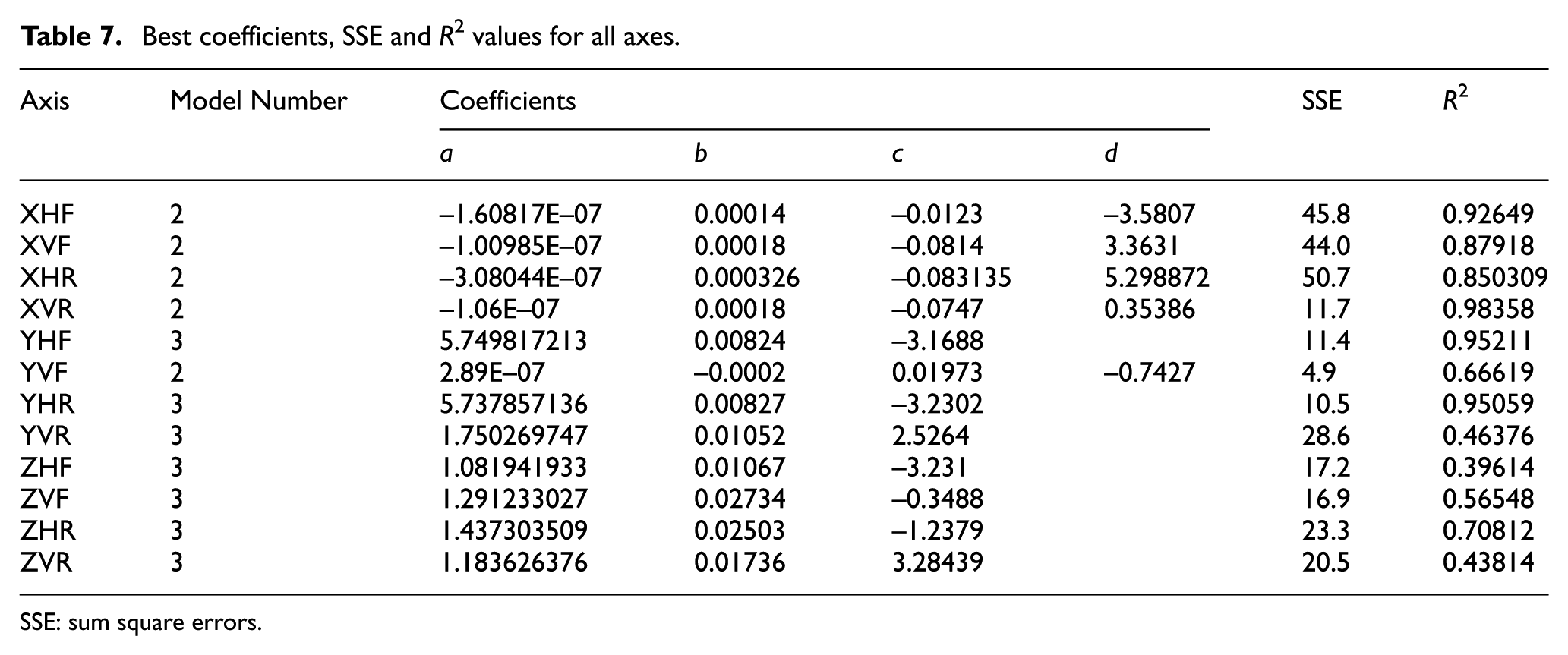
SSE: sum square errors.

Figure 4.

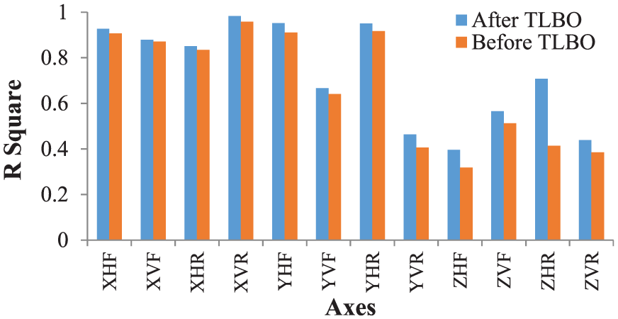
Comparison of R square—before and after the implementation of TLBO.

Figure 5.

Nominal positions versus error—X-axis.

Conclusion

The positional errors have been measured in an equal interval by varying the nominal position of X, Y and Z axes using laser interferometer in CNC VMC both in forward and reverse direction. Different mathematical models have been developed for the measured error and the best model has been selected for each axis using the AIC method. The selected best model’s coefficients were optimized by implementing TLBO algorithm with the objective of minimizing SSE and maximizing R². TOPSIS method has been adapted to convert the dual objectives into a single objective. A value of 1%–2.6% of improvement in R² value in X-axis, 1%–14.3% in Y-axis and 10.3%–71.1% in Z-axis were observed in this proposed method.

The contribution of the authors in this present work is aimed to develop a mathematical model by minimizing the SSE and maximizing the R² values to calculate position errors presented in CNC machine tools in X, Y and Z axes both in forward and reverse direction, using the error data measured by laser interferometer as per VDI 3441 Germany standard which can’t be entirely eliminated from the machineries. Limitations of the paper are the developed model in the present work is suitable only to determine the position errors presented in the CNC machine tools based on the error data measured by laser interferometer as per VDI 3441 Germany standard, and the thermal errors are not considered in the present work.

Footnotes

Acknowledgements

The authors would like to express their most profound appreciation and sincere thanks to Shri VAP Sharma, Mrs S Sudha, Shri SS Avadhani, Mr CT Shivaraj and Mr Ramamohan of Central Manufacturing Technology Institute, Bangalore, for their kind support in positioning error measurements using laser interferometer.

Declaration of conflicting interests

The author(s) declared no potential conflicts of interest with respect to the research, authorship and/or publication of this article.

Funding

The author(s) received no financial support for the research, authorship and/or publication of this article.

ORCID iD

Jamuna Ravichandran

References

Vinod

Narendra Reddy

Sajin

Real-time positioning error compensation for a turning machine using neural network. Proc Mat Sci 2014; 5: 2293–2300.

Ramesh

Mannan

Poo

AN.

Error compensation in machine tools—a review: part I: geometric, cutting-force induced and fixture-dependent errors. Int J Mach Tool Manu 2000; 40: 1235–1256.

Dave

Khandare

Mehta

JP.

Accuracy enhancement of 3 axis vertical milling machine centre. In: Proceedings of the 1st international and 16th national conference on machines and mechanisms (iNaCoMM2013), IIT Roorkee, Roorkee, India, 18–20 December 2013, pp. 953–956.

Liu

Xue

Tan

Backlash error measurement and compensation on the vertical machining center. Engineering 2010; 2: 403–407.

Naveen Kumar

Darshan Kumar

Rachappa

CT.

Condition monitoring of CNC machine tool accuracy with Renishaw equipment. Int J Innov Res Sci Eng Tech 2013; 2(12): 7861–7866.

Fines

Agah

Machine tool positioning error compensation using artificial neural networks. Eng Appl Artif Intel 2008; 21: 1013–1026.

Mahdavinejad

RA.

Prediction of angular errors on a vertical CNC Milling machine. Iran J Sci Technol B 2011; 35: 181–195.

El Ouafi

Guillot

Bedrouni

. Accuracy enhancement of multi-axis CNC machines through online neuro compensation. J Intell Manuf 2000; 11: 535–545.

Tan

Huang

Lim

, et al. Geometrical error modeling and compensation using neural networks. IEEE T Syst Man Cy C 2006; 36(6): 797–809.

10.

Han

Jin

Liu

, et al. A review of geometric error modeling and error detection for CNC machine tool. Appl Mech Mater 2013; 303–306: 627–631.

11.

Kopac

Pusavec

Kramar

. How to improve the positional accuracy of HSC machine tools. In: 7th Brazilian congress on manufacturing engineering, 2013, pp. 1–10.

12.

Begovic

Plancic

Ekinovic

, et al. Laser interferometry- measurement and calibration method for machine tools. In: 3rd conference “MAINTENANCE 2014,”Zenica, Bosnia and Herzegovina, 11–13 June 2014, pp. 19–25.

13.

Barman

Sen

Enhancement of accuracy of multi-axis machine tools through error measurement and compensation of errors using laser interferometry technique. Mapan 2010; 25(2): 79–87.

14.

Wan

Liu

Zhang

A new algorithm for the identification of CNC geometric errors. Proc Cirp 2016; 56: 293–298.

15.

Jung

J-H

Choi

J-P

Lee

S-J.

Machining accuracy enhancement by compensating for volumetric errors of a machine tool and on-machine measurement. J Mater Process Tech 2006; 174: 56–66.

16.

Bryan

JB.

A simple method for testing measuring machines and machine tools Part 1: principle and application. Precis Eng 1982; 4(3): 61–69.

17.

Ekinovic

Prcanovic

Begovic

Calibration of machine tools by means of laser measuring systems. Asian Trans Eng 2013; 2(6): 17–21.

18.

Zhang

Chu

Yang

. Research of error detection and compensation of CNC machine tools based on laser Interferometer. In: 2015 2nd international conference on machinery, materials engineering, chemical engineering and biotechnology, 2015, pp. 285–289.

19.

Lei

Hsu

YY.

Accuracy test of five-axis CNC machine tool with 3D probe ball. Part I: design and modeling. Int J Mach Tool Manu 2002; 42: 1153–1162.

20.

Lei

Hsu

YY.

Accuracy test of five-axis CNC machine tool with 3D probe ball. Part II: error estimation. Int J Mach Tool Manu 2002; 42: 1163–1170.

21.

Lei

Hsu

YY.

Accuracy enhancement of five-axis CNC machines through real-time error compensation. Int J Mach Tool Manu 2003; 43: 871–877.

22.

Lei

Hsu

YY.

Error measurement of five-axis CNC machines with 3D probe ball. J Mater Process Tech 2003; 139: 127–133.

23.

Zargarbashi

SHH

Mayer

. Assessment of machine tool trunnion axis motion error, using magnetic double ball bar. Int J Mach Tool Manu 2006; 46: 1823–1834.

24.

Wang

Griffin

BA.

Noncontact laser technique for circular contouring accuracy measurement. Rev Sci Instrum 2001; 72: 1594–1596.

25.

Wang

Laser vector measurement technique for the determination and compensation of volumetric positioning errors. Part I: basic theory. Rev Sci Instrum 2000; 71: 3933–3937.

26.

Wang

Laser vector measurement technique for the determination and compensation of volumetric position errors. Part II: experimental verification. Rev Sci Instrum 2000; 71: 3938–3941.

27.

www.Renishaw.com

28.

Xiang

Yang

Using a double ball bar to measure 10 position dependent geometric errors for rotary axes on five-axis machine tools. Int J Adv Manuf Tech 2014; 75: 559–572.

29.

Xiang

Yang

Using a double ball bar to identify position dependent geometric errors for rotary axes on five axis machine tools. Int J Adv Manuf Tech 2014; 70(9): 2071–2082.

30.

Gohel

Makwane

AH.

Integrated geometric errors simulation, measurement and compensation of vertical machining centers. Int J Adv Manuf Tech 2014; 4(1): 21–26.

31.

Wan

Maropolous

PG.

Real-time error compensation of a three-axis machine tool using a laser tracker. Int J Adv Manuf Tech 2013; 69(1–4): 919–933.

32.

Yang

Yao

, et al. Modeling approach of regression orthogonal experiment design for the thermal error compensation of a CNC turning center. J Mater Process Tech 2002; 129: 619–623.

33.

Yang

Lee

Measurement and prediction of thermal errors of a CNC machining center using two spherical balls. J Mater Process Tech 1998; 75: 180–189.

34.

Hao

Hongtao

Qianjian

, et al. Thermal error optimization modeling and real-time compensation on CNC turning center. J Mater Process Tech 2008; 207: 172–179.

35.

Akaike

A new look at the statistical model identification. IEEE T Automat Contr 1974; 19: 716–723.

36.

Akaike

Factor analysis and AIC. Psychometrika 1987; 52: 317–332.

37.

Bozdogan

Akaike’s Information Criterion and recent developments in information complexity. J Math Psychol 2000; 44: 62–91.

38.

Wang

Liu

Comparison of Akaike Information Criterion (AIC) and Bayesian Information Criterion (BIC) in selection of stock–recruitment relationships. Fish Res 2006; 77: 220–225.

39.

Kuha

AIC and BIC: comparisons of assumptions and performance. Sociol Method Res 2004; 33: 188–229.

40.

Mazerolle

MJ.

Improving data analysis in herpetology: using Akaike’s Information Criterion (AIC) to assess the strength of biological hypotheses. Amphibia-Reptilia 2006; 27: 169–180.

41.

Mahbub Latif

AHM

Zakir Hossain

Ataharul Islam

Model selection using modified Akaike’s Information Criterion: an application to maternal morbidity data. Austrian J Stat 2008; 37(2): 175–184.

42.

Rao

Savsani

Vakharia

DP.

Teaching–learning-based optimization: a novel method for constrained mechanical design optimization problems. Comput Aided Design 2011; 43: 303–315.

43.

Rao

Kalyankar

VD.

Multi-pass turning process parameter optimization using teaching–learning-based optimization algorithm. Sci Iran Trans E 2013; 20(3): 967–974.

44.

Crepinsek

Liu

S-H

Mernik

A note on teaching–learning-based optimization algorithm. Inform Sciences 2012; 212: 79–93.

45.

Venkatas Rao

. Review of applications of TLBO algorithm and a tutorial for beginners to solve the unconstrained and constrained optimization problems. Deci Sci Let 2016; 5: 1–30.

46.

Rao

KC.

Advanced optimal tolerance design of machine elements using teaching–learning-based optimization algorithm. Prod Manu Res 2014; 2(1): 71–94.

47.

Venkata Rao

. Simultaneous optimal selection of design and manufacturing tolerances with different stackup conditions using TLBO algorithm. In: International conference on innovations in engineering and technology (ICIET’2013), Bangkok, Thailand, December 2013 pp. 25–26.

48.

Satapathy

Naik

Parvathi

A teaching learning-based optimization based on orthogonal design for solving global optimization problems. SpringerPlus 2013; 2: 130.

49.

Venkata Rao

Patel

. An improved teaching–learning-based optimization algorithm for solving unconstrained optimization problems. Sci Iran 2013; 20(3): 710–720.

50.

Jahanshahloo

Lofti

Izadikhah

An algorithmic method to extend TOPSIS for decision-making problems with interval data. Appl Math Comput 2006; 175: 1375–1384

51.

Jadidi

Hong

Firouzi

, et al. TOPSIS and fuzzy multi-objective model integration for supplier selection problem. J Achiev Mater Manuf Engg 2008; 31(2): 762–769.

52.

Hung

Chen

LH.

A fuzzy TOPSIS decision making model with entropy weight under intuitionistic fuzzy environment. Proc Inter Multi-Conf Eng Comp Sci 2009; 1: 1–4.

53.

Pitt

From laboratory to on-line measurement and control. Meas Control 1998; 31(7): 196–201.

54.

Mahapatra

Thareja

Kaur

, et al. A machine vision system for tool positioning and its verification. Meas Control 2015; 48(8): 249–260.

55.

Zhou

Sensorless balance method for the spindle system of computer numerical control gear grinding machine. Meas Control 2018; 51(9): 460–469.

56.

Luo

Liu

, et al. Analysis and compensation of equivalent diameter error of articulated arm coordinate measuring machine. Meas Control 2018; 51: 16–26.

57.

Katebi

Lee

Roux

EASY5 application in process modeling optimization and central. Measure Cont 1992; 25(7): 207–212.

58.

Jamuna

Natarajan

Muruganandham

Investigation of backlash error on the vertical machining centre using artificial neural network. Res India Publ 2016; 11(3): 449–454.

Measurement of error in computer numerical control machines and optimization using teaching–learning-based optimization algorithm

Abstract

Keywords

Introduction

Problem definition

Methodology

Measurement of error in nominal position of axes

Development of mathematical model

Selection of the best mathematical model

Optimization of coefficients of the best model

TLBO algorithm

Conversion of dual objectives into single objective using TOPSIS method

Implementation of TOPSIS method and TLBO algorithm

Result and discussion

Conclusion

Footnotes

Acknowledgements

Declaration of conflicting interests

Funding

ORCID iD

References