Robust and adaptive control design of a drilling rig during the operating modes

Abstract

Oil well drilling towers have different operating modes during a real operation, like drilling, tripping, and reaming. Each mode involves certain external disturbances and uncertainties. In this study, using the nonlinear model for the modes of the operation, robust and/or adaptive control systems are designed based on the models. These control strategies include five types of controllers: cascaded proportional–integral–derivative, active disturbance rejection controller, loop shaping, feedback error learning, and sliding mode controller. The study presents the design process of these controllers and evaluates the performances of the proposed control systems to track the reference signal and reject the uncertain forces including the parametric uncertainties and the external disturbances. This comparison is based on the mathematical performance measures and energy consumption. In addition, three architectures are presented to control the weight on bit during drilling process, and also to maintain a preset constant weight on bit, two control approaches are designed and presented.

Introduction

A drilling rig is a machine that digs boreholes in the ground. The drilling machine has different equipment like actuator, draw-works, traveling block or hook, mud pump, top-drive, drill string, and bottom-hole-assembly (BHA). Dynamic modeling of these equipment constitutes the basis for system analysis and control. The model has to describe the system’s behavior during operating modes in real wells and it has to be simple enough for analysis and control purposes. On the other hand, as the model uncertainties (structured and/or unstructured) have strong effects on the nonlinear control systems, ¹ the robust and/or adaptive control architectures can be applied to deal with model uncertainties. The general schematic of a drill rig and its main equipment are illustrated in Figure 1.

Figure 1.

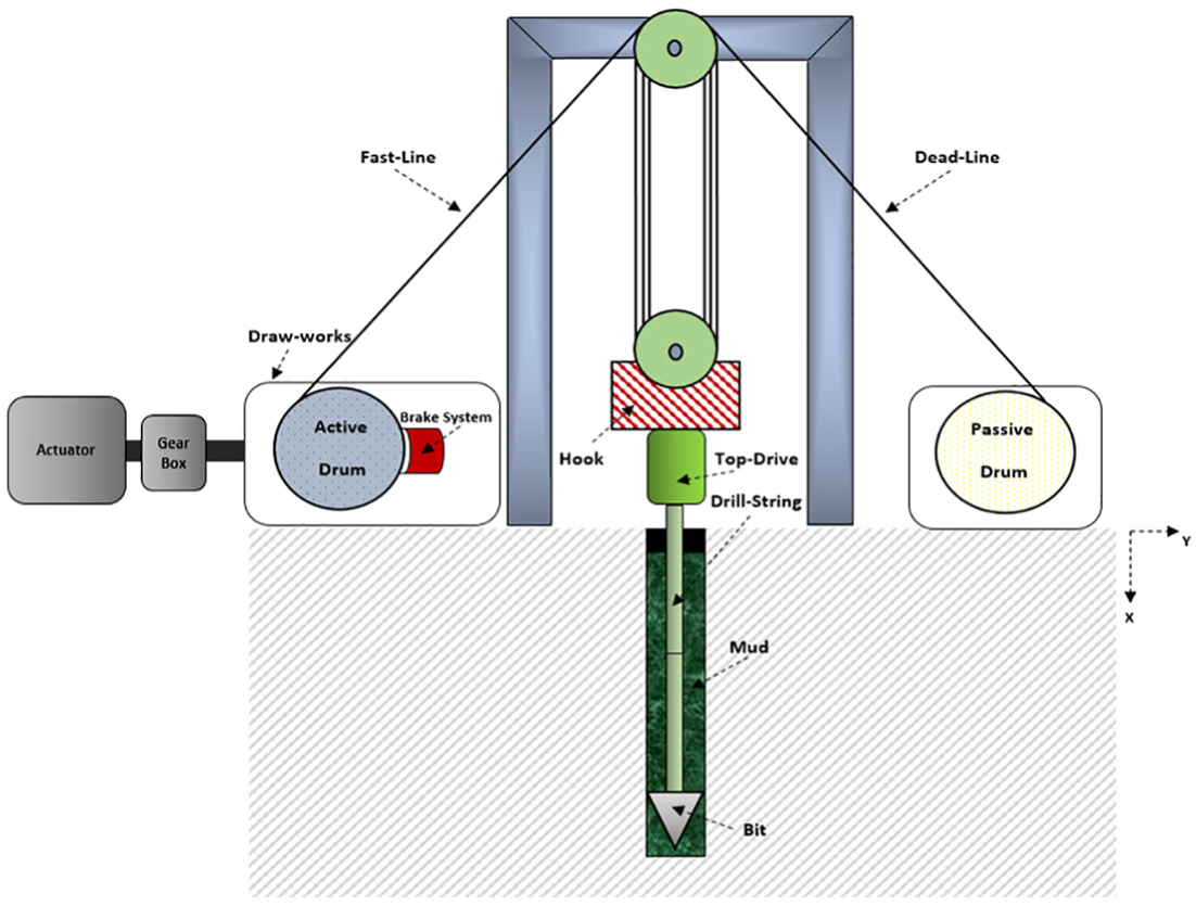
General schematic of a drilling rig.

The towers have different operating modes during a real operation. During tripping operation, the drill string removes the entire drill string from the wellbore and then runs it back in. Drilling operation is the cutting process that uses a bit to dig a hole in the ground. The process of enlarging the hole is called reaming. It is similar to downward tripping, just the top-drive and the bit continue to rotating without having any rock-bit interaction. During the tripping process, there is just need for position control of the drill string. The vertical velocity reference is given through a joystick by the operator, and the position reference can be easily set by him. Drilling action comprises two processes: rotational motion of the drill string and the vertical penetration of the bit. During this operation, the rate of penetration (ROP) as the vertical velocity reference is set to the system, while some other drilling parameters like weight on bit (WOB) must be controlled. In addition, each of the operating modes involves certain external disturbances and uncertainties. Actually, these annoying forces generate variable loadings on the actuators.

Over the last half-century, wide research effort has been conducted to mathematically model and control the drilling rig. The motion control approaches and optimization methods have been studied previously. Some articles address the issue of motion control problems generally, and some of them present the motion control architectures particularly in the drilling rigs. A class of motion control problems is addressed in a study, ² which applies a conventional proportional–integral–derivative (PID) controller, and two alternative control algorithms: loop-shaping and linear active disturbance rejection controller (ADRC). The study evaluates the control systems’ ability to reject the disturbances. Sabanovic and Ohnishi ³ are concerned with the design methods for faster and more accurate control of mechanical motion. It presents the solution of complex problems in motion control systems. After introducing the basics of electromechanical systems and control system design, some issues in motion control such as acceleration control, disturbance observer, interactions, and constraints are presented. Kolpak and Ivanov ⁴ developed a nonlinear mathematical model of drilling rig system, consisting of the rig, the control cabin, the working platform, and platforms with engines. The rig system has 6 degrees of freedom, and the mathematical model is presented by a system of nonlinear ordinary differential equations. The mathematical model in the study by Leonard ⁵ presents the equations of motion that simulate the fundamental behavior of the drill string during both rotary and slide drilling operations. Design of control approaches for the vertical drilling operation is studied by Shah. ⁶ The author presents a robust servo controller design, based on the existing mathematical models of drill string systems and rock cutting process that successfully tracks the reference vertical motion velocity. Saldivar ⁷ presents a model to describe the behavior of the drill string during drilling operation and control design for the stabilization of the drilling system. In the study by Ritto et al., ⁸ the drill string is modeled using a bar model (tension, compression) and is discretized by means of the finite element method. In another article, ⁹ to avoid different bit sticking problems present in a conventional vertical drill string, a dynamical sliding mode control is presented. As the author mentions, the closed-loop system has two discontinuity surfaces. One of them gives rise to self-excited bit stick-slip vibrations and the other surface is introduced to perform the control goal despite variations in the WOB and the other system parameters. The article ¹⁰ presents a fuzzy logic controller to drill string motion. This control approach assures simultaneously the high ROP and an acceptable level of stress in the drill string to increase its lifetime. Another study ¹¹ presents a model to analyze dynamic drill string behavior, estimate local contact forces, and predict the effect of different tripping velocity profiles on longitudinal and lateral contact forces. A thesis work ¹² investigates the potential for closed-loop feedback control on a large rotary electric blast-hole drill. The proposed control strategy is a proportional-integral-velocity (PIV) control. Model of hook load during tripping operation is addressed in the study by Kristensen. ¹³ The initial goal of the study is to evaluate and develop the mathematical model of the weight of the drill string when pulling it out of the hole. The first objective of the paper ⁷ is to find a model to describe the behavior of the rod during drilling operation, and the second objective is the control design for the stabilization of the drilling system through Lyapunov theory based on two different approaches: neutral-type time-delay model and wave equation model. In a research, challenges of modeling drilling systems are considered for the purposes of automation and control. ¹⁴ The author mentions that many studies are being made to develop models of the rig systems, drill string, and rock-bit interaction, but bringing all these models together in any unified manner and proposing a unified control solution to fully automate the whole process is still an exploratory venture. The paper by Kruljac et al. ¹⁵ helps engineers to understand various mechanisms and variables that affect BHA’s behavior, like weight-on-bit, rotary speed, and penetration rate. The paper proposes analytical method for calculating side forces and contact points. The proposed method provides the capability to evaluate and to adjust the actual well profile in an interactive, real-time mode, thus enabling well-path steering. A study by Dashevskiy et al. ¹⁶ presents a control system for predictive control in drilling optimization. A measurement while drilling (MWD) dynamics measurement tool is a required component of a closed-loop drilling control system. This work presents the initial field-test results of a control system that uses a neural network for predictive control in drilling optimization. A model for ROP estimation based on the Bourgoyne & Young’s model (BYM) is presented in directional and horizontal wells. ¹⁷ This study aims to propose an ROP model considering many drilling parameters and conditions. Another similar study ¹⁸ researches the BYM formulation, how it is applied in terms of ROP modeling, and identifies the main drilling parameters driving each sub-function. Another article ¹⁴ shows the issue of drill string dynamics, modeling and controlling of rock-bit interaction, and ROP optimization, through standard industry communication speeds at multiple points along the wellbore.

The optimization process of drilling parameters has direct effects on the cost reduction, which aims to optimize controllable variables during drilling operation such as WOB and bit rotation speed for obtaining maximum drilling rate. Determination of optimum WOB is very important in drilling operation as this parameter can be changed during drilling operation. The study by Eren and Ozbayoglu ¹⁹ works with numerical correlations using the drilling parameters to observe their effects to the ROP. In a project, ²⁰ Bourgoyne & Young’s ROP model has been selected to study the effects of several parameters during drilling operation. The penetration model for the field is constructed using the results from statistical method.

Real-time drilling optimization that relies solely on surface data has proven ineffective because it does not take into account the behavior of the BHA downhole. Two solutions to acquire the data of BHA are generally presented: measure them practically by sensors or predict them. To measure and acquire the data from BHA and analyze them to use in the controllers, some studies present the methods and approaches to measurement while drilling or MWD systems. A previous work ²¹ clarifies that MWD refers to the acquisition and collection of wellbore deviation directional surveys; the acquisition and collection of drilling mechanics data, like downhole torque, pressure, or vibration; and the process of sending the data up-hole in real time. Another paper ²² presents an overview of the applications of the measurements performed by the MWD tools. An evaluation of the available telemetry techniques used to transfer the measured data from the downhole tools to surface is performed. A previous study ²³ mentions the reliable, precise, and efficient downhole MWD systems as key prerequisites for accurate well placement with an optimal ROP. In the application, ²⁴ it is shown that by sending a pulse into the hole with fluid, the sensor output helps determine response characteristics such as pressure based on the feedback from pulses such as depth, material composition, and thus optimize how the drill speed or drill bit should be modified based on the measurements and material. Ertas et al. ²⁵ present the methods to estimate severity of downhole vibration for a wellbore drill tool assembly. The estimation of downhole vibration index is implemented by evaluating the determined surface vibration attribute with respect to the identified reference surface vibration attribute. The paper by Klotz et al. ²⁶ presents a system for downhole-to-surface mud pulse telemetry (MPT). Since the pipe bore is filled with flowing drilling mud, this system is able to handle the complex and continuously varying properties of the transmission channel by optimizing the transmission signal and the surface processing algorithms in real time. El-Biblawi et al. ²⁷ mention that drilling specific energy has been determined in all types of rocks under investigation at different applied loads and rotary speeds. The results have been obtained for ROP to show the variation in specific energy with the different rocks.

The autonomous drilling system is designed to provide a constant drilling state at the bit. ²⁸ These states can be the WOB, the ROP, the pressure difference in the drill string (Delta P), and the torque of the top-drive, which are well known as the modes of the autonomous drilling. The principal advantage of the autonomous drilling is to provide a system, which is able to improve the efficiency of drilling operations through controlling of the drilling rig’s equipment. The autonomous drilling modes can be activated individually or in combination with other modes to form the optimum drilling control. A study examines and defines drilling systems’ automation, its drivers, enablers and barriers, and its current state and goals. ²⁹ In particular, it studies the drilling systems’ automation among all segments of the drilling industry. Vishnumolakala ³⁰ develops a simulation environment, models an automatic managed pressure drilling using constant BHA pressure technique by a PID controller, and optimizes the drilling operations. An invention describes a method for the autonomous drilling of ground holes by a drill rig. ³¹ The method includes the step of utilizing an autonomous drilling procedure in order to control the drilling equipment to dig a hole after locating the drill rig in a ground position where the well must be drilled.

In this study, using the existing nonlinear models for the vertical and rotational motions of drill string and drill bit during the operating modes, five different types of motion controllers are designed. These robust and/or adaptive control systems include cascaded proportional–integral–derivative (CPID), active disturbance rejection, loop shaping, feedback error learning (FEL), and sliding mode. The ability of the robust and adaptive controllers has been utilized to dealing with uncertain forces on the system, including the structured or parametric model uncertainties and the external disturbances. The design process of each control system is presented in detail and then the performances of them are compared based on the simulation results, the mathematical performance measures, and the energy consumptions. On the other hand, three control architectures are presented to constrain the WOB during drilling process, such a way not exceed a determined value. Also, to maintain a preset constant WOB, known as WOB mode in autonomous drilling, two control approaches are designed and presented.

The main purpose of this paper is to design and evaluate five types of control algorithms on the advanced dynamical model of the drilling rig including external disturbances and parametric uncertainties. As far as we have seen in the literature, several controllers such as PID, ADRC, and the sliding mode control have been used for the control of the drilling rigs. In addition, we have designed the loop-shaping and FEL type controllers. Also, to our knowledge, there is hardly any literature that evaluates and makes a comprehensive comparison of the control systems on advanced models using mathematical measures. This contribution reveals novelty for the design of drilling rigs in the theoretical domain. The second purpose is to control the WOB, based on the realistic conditions or constraints in the field, and the optimum values.

Dynamic modeling

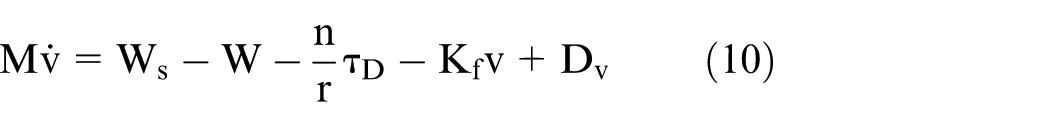
Dynamic modeling of the drilling rig equipment constitutes the basis for system analysis and control. Draw-works and top-drive actuators, hoisting system, mud effect, drilling and cutting process, drill string, and BHA, are the important equipment in a drilling rig, which must be modeled mathematically. The governing equations for the motion of a drill string and drill bit, as presented in many works,^6,32,33 are as follows

$$\mathrm{M}\stackrel{·}{\mathrm{v}}={\mathrm{W}}_{\mathrm{s}}-\mathrm{W}-\frac{\mathrm{n}}{\mathrm{r}}{\mathrm{\tau }}_{\mathrm{D}}-{\mathrm{K}}_{\mathrm{f}}\mathrm{v}+{\mathrm{D}}_{\mathrm{v}}$$

(1)

$$\mathrm{I}\stackrel{·}{\omega }+\mathrm{c}\mathrm{\omega }={\tau }_{\mathrm{T}}-\mathrm{T}+{\mathrm{D}}_{\omega }$$

(2)

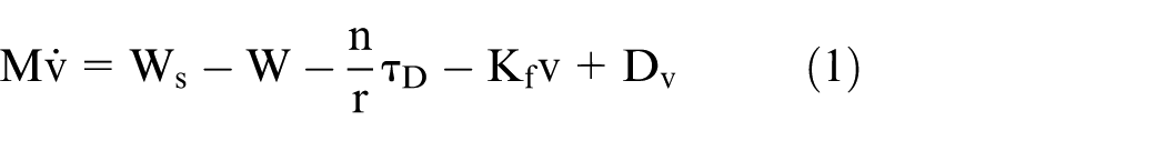
In equation (1), which describes the vertical motion of drill string, the variable “v” is the vertical velocity, the variable “W” is the WOB, the variable ${\mathrm{W}}_{\mathrm{s}}={\mathrm{m}}_{\mathrm{H}}·\mathrm{g}·\mathrm{BF}$ is the submerged weight, where the variable “m_H” is mass of the hook load and “BF” is the Buoyancy factor, the constant “n” is the number of times the cable wrapped around the sheave, the variable “r” is the radius of the drum, “τ_D” is the torque applied by the draw-works motor, the constant “K_f” is the coefficient of mud viscous friction, the variable $\mathrm{M}={\mathrm{m}}_{\mathrm{H}}+({\mathrm{n}}^2/{\mathrm{r}}^2){\mathrm{I}}_{\mathrm{d}}$ , the variable “I_d” is the inertia of the drum, and “D_v” is the external disturbance effecting on the vertical motion. As a novelty, we have considered the radius of the drum “r,” and consequently some other parameters, as the variables not the constant values. This is because of changing length of the cable, which is wrapped around the drum. Based on the illustrated Figure 2, $\mathrm{r}={\mathrm{R}}_1+{\mathrm{R}}_{(\mathrm{x})}$ , where ${\mathrm{R}}_{(\mathrm{x})}$ is a function of the hook position “x” and can be calculated as below equation (3), where “r_c” is the radius of the cable, “R₁”is the outer radius of the cylinder, and “i” and “j” are number of columns and rows of cable wrapped on the cylinder

$${\mathrm{R}}_{\left(\mathrm{x}\right)}=\{\begin{array}{cc}\begin{array}{c}\begin{array}{c}\dots \hfill \\ \multicolumn{1}{c}{(\mathrm{j}-1)·2·{\mathrm{r}}_{\mathrm{c}}}\end{array}\hfill \\ \multicolumn{1}{c}{\mathrm{j}·2·{\mathrm{r}}_{\mathrm{c}}}\\ \multicolumn{1}{c}{\begin{array}{c}(\mathrm{j}+1)·2·{\mathrm{r}}_{\mathrm{c}}\hfill \\ \multicolumn{1}{c}{\dots }\end{array}}\end{array}\hfill & \begin{array}{c}\begin{array}{c}\dots \hfill \\ \multicolumn{1}{c}{\begin{array}{cc}\mathrm{if}\hfill & 0<x\le \frac{2\pi i·({\mathrm{R}}_1+(\mathrm{j}-1))·2·{\mathrm{r}}_{\mathrm{c}}}{\mathrm{n}}\hfill \end{array}}\end{array}\hfill \\ \multicolumn{1}{c}{\begin{array}{cc}\mathrm{if}\hfill & -\frac{2\pi i·({\mathrm{R}}_1+\mathrm{j})·2·{\mathrm{r}}_{\mathrm{c}}}{\mathrm{n}}<x\le 0\hfill \end{array}}\\ \multicolumn{1}{c}{\begin{array}{cc}\mathrm{if}\hfill & \begin{array}{c}-2·\frac{2\pi i·({\mathrm{R}}_1+(\mathrm{j}+1))·2·{\mathrm{r}}_{\mathrm{c}}}{\mathrm{n}}<x\le -\frac{2\pi i·({\mathrm{R}}_1+(\mathrm{j}+1))·2·{\mathrm{r}}_{\mathrm{c}}}{\mathrm{n}}\hfill \\ \multicolumn{1}{c}{\dots }\end{array}\hfill \end{array}}\end{array}\hfill \end{array}$$

(3)

Figure 2.

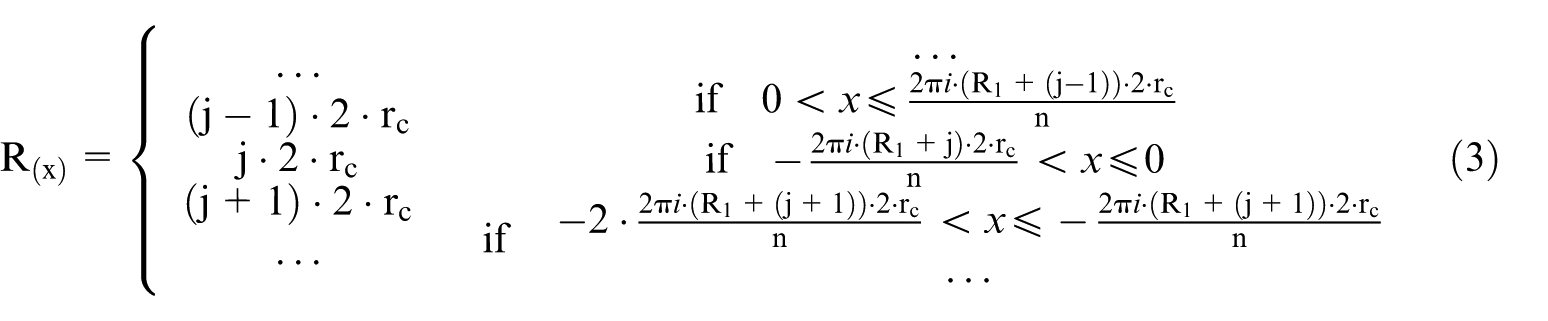
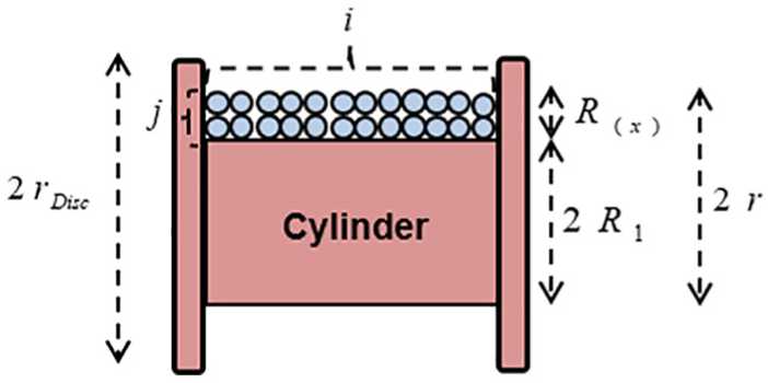
Draw-works drum model.

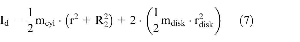
The parameters which depend on the radius of the drum, and thus functions of the hook position “x,” can be calculated as equations (4)–(7), where “m_pipes” is mass of the pipes on the drill string, “m_T” is mass of the top-drive, “m_ca” is mass of the cable, “m_cyl” is mass of the cylinder, “m_ca0” is mass of the cable at initial time, “m_cyl0” is mass of the cylinder at initial time, “m_cal” is mass of the cable with length of 1 m, “m_disk” is mass of the disk, “r_disk” is radius of the disk, and “R₂” is the inner radius of the cylinder

$${\mathrm{m}}_{\mathrm{H}}={\mathrm{m}}_{\mathrm{pipes}}+{\mathrm{m}}_{\mathrm{T}}+{\mathrm{m}}_{\mathrm{ca}}$$

(4)

$${\mathrm{m}}_{\mathrm{ca}}={\mathrm{m}}_{\mathrm{ca}0}+\mathrm{n}·\mathrm{x}·{\mathrm{m}}_{\mathrm{ca}1}$$

(5)

$${\mathrm{m}}_{\mathrm{cyl}}={\mathrm{m}}_{\mathrm{cyl}0}-\mathrm{n}·\mathrm{x}·{\mathrm{m}}_{\mathrm{ca}1}$$

(6)

$${\mathrm{I}}_{\mathrm{d}}=\frac{1}{2}{\mathrm{m}}_{\mathrm{cyl}}·({\mathrm{r}}^2+{\mathrm{R}}_2^2)+2·(\frac{1}{2}{\mathrm{m}}_{\mathrm{disk}}·{\mathrm{r}}_{\mathrm{disk}}^2)$$

(7)

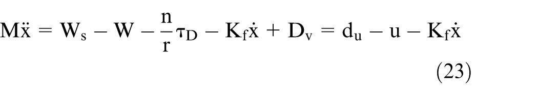
In equation (2), which describes the rotational motion of drill string, the variable “ω” is the rotational velocity, the variable “I” is the moment of inertia of drill string and BHA, the variable c is the torsional stiffness of the drill string, “τ_T” is the torque applied by the top-drive, the variable “T” is the torque on bit, and “D_ω” is the external disturbance effecting on the rotational motion. During the drilling operation, the variables, WOB and torque on bit, are calculated as^6,32,33

$$\mathrm{W}=2\pi \mathrm{a}\xi \epsilon \frac{\mathrm{v}}{\omega }$$

(8)

$$\mathrm{T}=\pi {\mathrm{a}}^2\epsilon \frac{\mathrm{v}}{\omega }$$

(9)

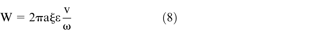
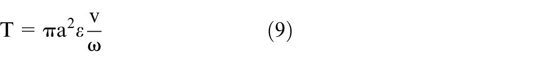
where the constant “a” is the bit radius, the constant “ξ” is the ratio of the vertical force to the horizontal force between rock and cutter contact surfaces, and the variable “ε” is the rock stiffness. During the tripping, reaming, and back reaming operations, the weight and torque on bit terms equal zero, as there is no rock-bit interaction. It is worth mentioning that, during the drilling, the WOB term will be limited, in such a way not exceeding a determined value as will be described in section “WOB controller,” and the torque on bit term will be eliminated as a disturbance from the system.

Controller design

The controlling process must be performed for all modes of operation, and for each operating mode, an appropriate controller must be designed. During each operating mode, position and/or velocity control must be performed by the controller. The control block diagram of the system is shown in Figure 3. In order to control the velocity of the hook during the operating modes, five control strategies are designed and implemented: cascade PID controller (CPID), active disturbance rejection controller (ADRC), loop shaping controller (LSC), feedback error learning controller (FEL), and sliding mode controller (SMC). The CPID, ADRC, and SMC controllers have been applied in many works and presented in the literature.^{6,9,12,30,34–39} The design of the LSC and FEL controllers applied on the model is another novelty of this work. The design process of all the controllers is described in detail.

Figure 3.

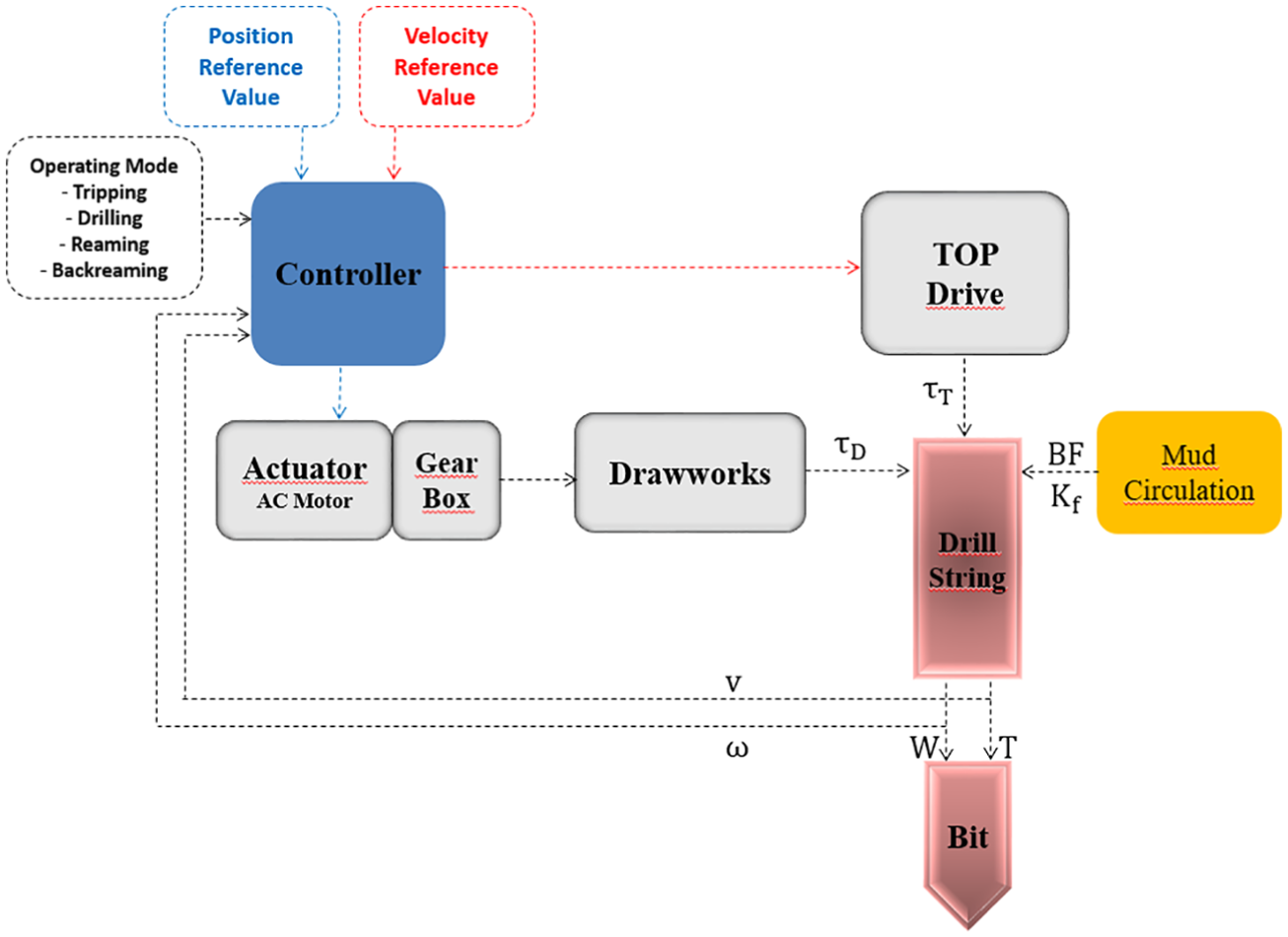
Control block diagram.

CPID controller

The CPID controller is mainly exerted to achieve fast rejection of disturbance before it propagates to the other parts of the plant. ⁴⁰ Figure 4 illustrates the simplest architecture of a cascade control, which involves two inner and outer control loops. The first PID controller in the outer loop is the primary controller that regulates the controlled variable (velocity) by setting the set-point of the inner loop. The second PID controller in the inner loop rejects disturbance ( $D_2$ ; acceleration) locally before it propagates to the plant. The tuning of both PID controllers are manually implemented and optimized to achieve the minimum tracking error; $\mathrm{e}={\mathrm{v}}_{\mathrm{ref}}-\mathrm{v}$ .

Figure 4.

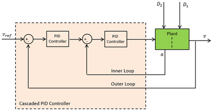
Structure of cascade PID controller.

ADRC controller

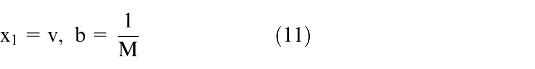
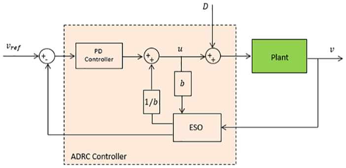
The architecture of the ADRC is illustrated in Figure 5. It consists of two main components: the proportional–derivative (PD) controller and the ESO (extended state observer). The designed ESO will eliminate all the uncertain forces effecting on the system. In other words, this controller can successfully track the reference signal while rejecting all the uncertainties and disturbances. Using the equation of vertical motion (equation (1)), the dynamics of the observer can be derived as follows

$$\mathrm{M}\stackrel{·}{\mathrm{v}}={\mathrm{W}}_{\mathrm{s}}-\mathrm{W}-\frac{\mathrm{n}}{\mathrm{r}}{\tau }_{\mathrm{D}}-{\mathrm{K}}_{\mathrm{f}}\mathrm{v}+{\mathrm{D}}_{\mathrm{v}}$$

(10)

$${\mathrm{x}}_1=\mathrm{v},\mathrm{b}=\frac{1}{\mathrm{M}}$$

(11)

Figure 5.

Structure of ADRC controller.

The effect of all uncertain forces (the external disturbances and the model parametric uncertainties) on the system is considered as a new state “x₂”

$${\stackrel{·}{\mathrm{x}}}_1=\mathrm{b}·({\mathrm{W}}_{\mathrm{s}}-\mathrm{W}-{\mathrm{K}}_{\mathrm{f}}.{\mathrm{x}}_1+{\mathrm{D}}_{\mathrm{v}}-\mathrm{u})={\mathrm{x}}_2-\mathrm{b}·\mathrm{u}$$

(12)

$${\stackrel{·}{\mathrm{x}}}_2=\mathrm{h}\approx 0$$

(13)

$$\left[\begin{array}{c}{\stackrel{·}{\mathrm{x}}}_1\hfill \\ \multicolumn{1}{c}{{\stackrel{·}{\mathrm{x}}}_2}\end{array}\right]=\left[\begin{array}{c}{\mathrm{x}}_2\hfill \\ \multicolumn{1}{c}{\mathrm{h}}\end{array}\right]+\left[\begin{array}{c}-\mathrm{b}\hfill \\ \multicolumn{1}{c}{0}\end{array}\right]·\mathrm{u}$$

(14)

$$\left[\begin{array}{c}{\stackrel{·}{\hat{\mathrm{x}}}}_1\hfill \\ \multicolumn{1}{c}{{\stackrel{·}{\hat{\mathrm{x}}}}_2}\end{array}\right]=\left[\begin{array}{c}{\hat{\mathrm{x}}}_2\hfill \\ \multicolumn{1}{c}{0}\end{array}\right]+\left[\begin{array}{c}-\mathrm{b}\hfill \\ \multicolumn{1}{c}{0}\end{array}\right]·\mathrm{u}+{\mathrm{L}}_{\mathrm{D}}·({\mathrm{x}}_1-{\hat{\mathrm{x}}}_1)$$

(15)

$${\mathrm{L}}_{\mathrm{D}}=\left[\begin{array}{cc}2{\omega }_0\hfill & {\omega }_0^2\hfill \end{array}\right]$$

(16)

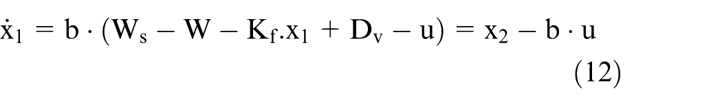
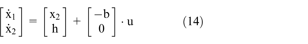
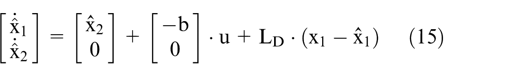
Equation (15) represents the observer dynamics. In equation (16), “ω₀” is the observer bandwidth, which can be derived by bandwidth parameterization as presented in the literature. ⁴¹

LSC controller

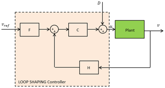
The LSC design method, also known as the frequency response-based controller design method, conceptually consists of two steps: convert all design specifications to loop gain constraints and find a controller to meet the specifications. The general structure of it is shown in Figure 6.

Figure 6.

Structure of loop-shaping controller.

Using the equation of vertical motion (equation (1)), first the transfer function of the plant is derived and then the transfer function of the controller can be achieved by the procedure, as presented in the literature. ⁴¹ Here, the effect of all uncertain forces (the external disturbances and the model parametric uncertainties) on the system is considered in term “d_u”

$$\mathrm{M}\stackrel{·}{\mathrm{v}}+{\mathrm{K}}_{\mathrm{f}}\mathrm{v}={\mathrm{W}}_{\mathrm{s}}-\mathrm{W}-\frac{\mathrm{n}}{\mathrm{r}}{\tau }_{\mathrm{D}}+{\mathrm{D}}_{\mathrm{v}}={\mathrm{d}}_{\mathrm{u}}-\mathrm{u}$$

(17)

$${\mathrm{G}}_{\mathrm{P}}=\frac{{\mathrm{V}}_{\left(\mathrm{s}\right)}}{{\mathrm{U}}_{\left(\mathrm{s}\right)}}=-\frac{1}{\mathrm{Ms}+{\mathrm{K}}_{\mathrm{f}}},{\mathrm{G}}_{\mathrm{F}}=1,{\mathrm{G}}_{\mathrm{H}}=1$$

(18)

$${\mathrm{G}}_{\mathrm{C}}=-{\left(\frac{\mathrm{s}+{\omega }_1}{\mathrm{s}}\right)}^{\mathrm{m}}·\frac{1}{\frac{\mathrm{s}}{{\omega }_1}+1}.\frac{1}{{(\frac{\mathrm{s}}{{\omega }_2}+1)}^{\mathrm{n}}}·{{\mathrm{G}}_{\mathrm{P}}}^{-1}$$

(19)

$${\omega }_{\mathrm{c}}=800\mathrm{rad}/\mathrm{s},{\omega }_1=\frac{{\omega }_{\mathrm{c}}}{2},{\omega }_2=2{\omega }_{\mathrm{c}}$$

(20)

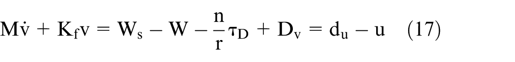
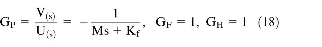
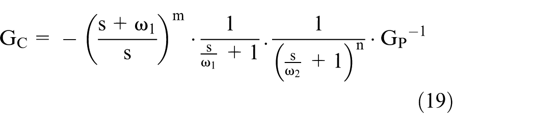
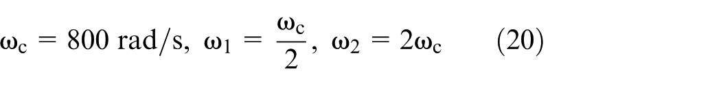
Equation (19) represents the controller transfer function. In equation (20), “ω_c” is the open-loop bandwidth, as presented in the literature. ⁴¹ Taking $\mathrm{m}=2$ and $\mathrm{n}=1$ , the controller will have 3 zeros and 4 poles. The Bode diagram of the open-loop system $({\mathrm{G}}_{\mathrm{P}}·{\mathrm{G}}_{\mathrm{C}})$ is illustrated in Figure 7. From the diagram, the gain and phase margins are roughly derived, $\mathrm{GM}\approx 70\mathrm{dB}$ and $\mathrm{PM}\approx {85}^{°}$ , which show a good stability in the closed-loop system. Using this controller, the step response of the closed-loop system $(({\mathrm{G}}_{\mathrm{P}}·{\mathrm{G}}_{\mathrm{C}})/(1+{\mathrm{G}}_{\mathrm{P}}·{\mathrm{G}}_{\mathrm{C}}))$ will be as shown in Figure 7.

Figure 7.

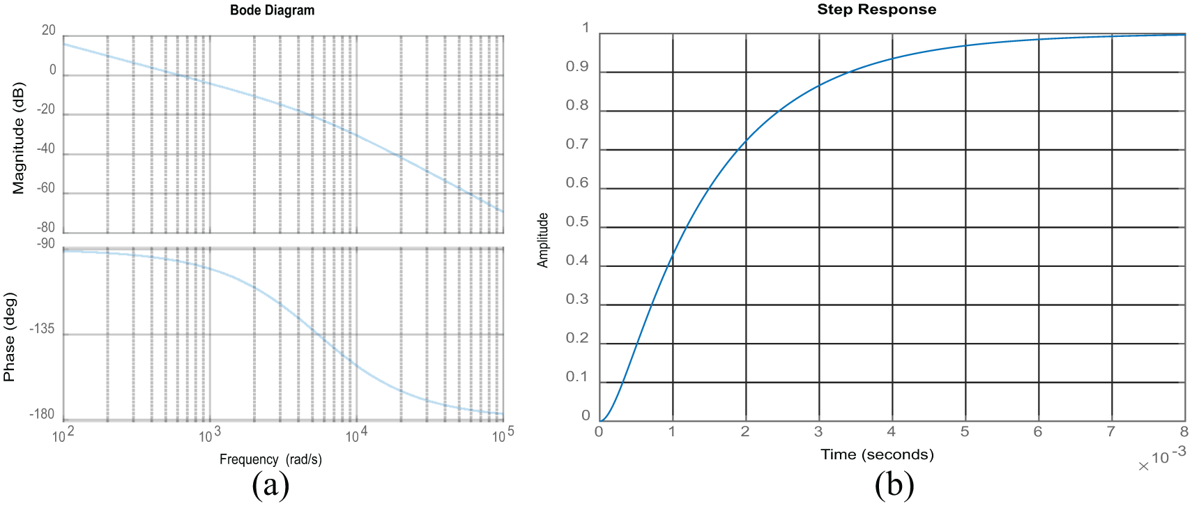
(a) Root locus and bode diagrams of the open-loop system and (b) step response of the closed-loop system.

FEL controller

The combination of a classic controller with an artificial neural network (ANN) is known as FEL as shown in Figure 8. Adaptive type of controller is used to handle the uncertainty due to the various extra annoying forces. Two types of FEL controllers are constructed and implemented; a PID controller is used (FEL1), and an ADRC controller is used (FEL2), as the classic controller.

Figure 8.

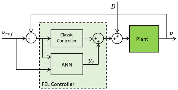
Structure of FEL controller.

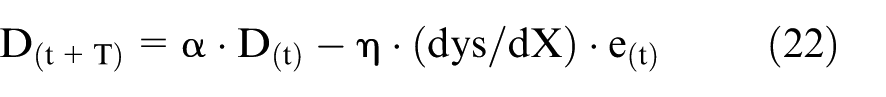
The FEL architecture is an adaptive control algorithm method,^42–44 which can easily eliminate the effect of the uncertain forces. The error signal that is obtained by the difference of the reference input and output is used for online training of the multi-layer perception (MLP) type of neural network with eight hidden layers.^42–44

The sigmoid activation functions are used in the ANN.^45–47 In addition to the error term, the reference input is processed in the ANN, as well. The output of the network contributes as the adaptive term. The number of the neurons in the hidden layer is equal to 8. ${\mathrm{X}}_{(\mathrm{t})}$ represents all the “states” of the network, namely the weights and all the parameters that are calculated during the learning process. “X_(t)” is updated according to an extended gradient rule as shown in equation (21). “y_s” is the output of the ANN and it is the adaptive part of the control input

$${\mathrm{X}}_{(\mathrm{t}+\mathrm{T})}={\mathrm{X}}_{\left(\mathrm{t}\right)}+\mathrm{\eta }·(\mathrm{dys}/\mathrm{dX})·{\mathrm{e}}_{\left(\mathrm{t}\right)}+{\mathrm{Z}}_{\left(\mathrm{t}\right)}$$

(21)

where $\mathrm{\eta }=3.8462\mathrm{e}-04$ is the learning rate, $\mathrm{dys}/\mathrm{dX}$ is the Jacobean matrix, $\mathrm{T}=2\mathrm{e}-04$ is the sampling time, and “Z_(t)” represents an additional contribution from a filtered error. The filter decay rate $\mathrm{\alpha }=0.02$ is called “momentum”

$${\mathrm{D}}_{(\mathrm{t}+\mathrm{T})}=\mathrm{\alpha }·{\mathrm{D}}_{\left(\mathrm{t}\right)}-\mathrm{\eta }·(\mathrm{dys}/\mathrm{dX})·{\mathrm{e}}_{\left(\mathrm{t}\right)}$$

(22)

$${\mathrm{Z}}_{\left(\mathrm{t}\right)}=\mathrm{\alpha }·{\mathrm{D}}_{\left(\mathrm{t}\right)}$$

SMC controller

One of the simplest architectures to robust control is the so-called sliding mode control (SMC) methodology. ¹ It is able to eliminate the effect of the model parametric uncertainties and the external disturbances, as described in the following. The architecture of our SMC is illustrated in Figure 9.

Figure 9.

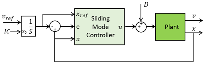
Structure of sliding mode controller.

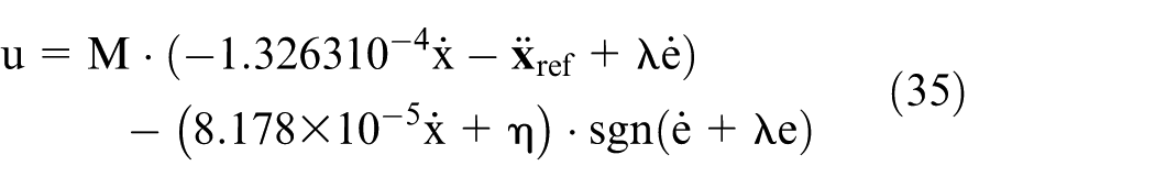
Based on the design procedure, presented in the mentioned reference, ¹ an SMC is designed to the vertical motion system. The dynamics of the vertical motion as presented previously is a second-order equation as follows

$$\mathrm{M}\stackrel{··}{\mathrm{x}}={\mathrm{W}}_{\mathrm{s}}-\mathrm{W}-\frac{\mathrm{n}}{\mathrm{r}}{\tau }_{\mathrm{D}}-{\mathrm{K}}_{\mathrm{f}}\stackrel{·}{\mathrm{x}}+{\mathrm{D}}_{\mathrm{v}}={\mathrm{d}}_{\mathrm{u}}-\mathrm{u}-{\mathrm{K}}_{\mathrm{f}}\stackrel{·}{\mathrm{x}}$$

(23)

$$\stackrel{··}{\mathbf{x}}={\mathrm{d}}_{\mathrm{u}}-\frac{{\mathrm{K}}_{\mathrm{f}}}{\mathrm{M}}\stackrel{·}{\mathrm{x}}-\frac{1}{\mathrm{M}}\mathrm{u}={\mathrm{d}}_{\mathrm{u}}-\alpha \stackrel{·}{\mathrm{x}}-\frac{1}{\mathrm{M}}\mathrm{u}$$

(24)

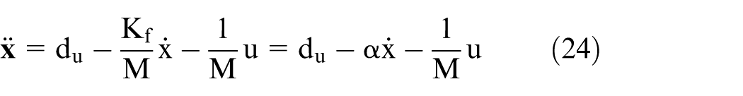
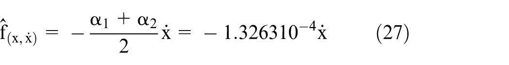
Here, the effect of the external disturbances is considered in term “d_u,” and the effect of the model parametric uncertainties in term “α.” Based on the number of pipes on the drill string, the constraints of “M” parameter can be achieved and then the constraints for term “α” will be calculated

$$9.328\times {10}^4\le \mathrm{M}\le 3.933\times {10}^5$$

(25)

$$5.0852\times {10}^{-5}={\mathrm{\alpha }}_1\le \mathrm{\alpha }\le {\mathrm{\alpha }}_2=2.144\times {10}^{-4}$$

(26)

The dynamics ${\mathrm{f}}_{(\mathrm{x},\stackrel{·}{\mathrm{x}})}=-\alpha \stackrel{·}{\mathbf{x}}$ is not exactly known, but estimated as equation (27), and the estimation error on ${\mathrm{f}}_{(\mathrm{x},\stackrel{·}{\mathrm{x}})}$ is assumed to be bounded by some known function ${\mathrm{F}}_{(\mathrm{x},\stackrel{·}{\mathrm{x}})}$ as equation (28). These two equations conclude equation (29)

$${\hat{\mathrm{f}}}_{(\mathrm{x},\stackrel{·}{\mathrm{x}})}=-\frac{{\mathrm{\alpha }}_1+{\mathrm{\alpha }}_2}{2}\stackrel{·}{\mathrm{x}}=-1.{326310}^{-4}\stackrel{·}{\mathrm{x}}$$

(27)

$$|{\hat{\mathrm{f}}}_{(\mathrm{x},\stackrel{·}{\mathrm{x}})}-{\mathrm{f}}_{(\mathrm{x},\stackrel{·}{\mathrm{x}})}|\le {\mathrm{F}}_{(\mathrm{x},\stackrel{·}{\mathrm{x}})}$$

(28)

$${\mathrm{F}}_{(\mathrm{x},\stackrel{·}{\mathrm{x}})}=8.178\times {10}^{-5}\stackrel{·}{\mathrm{x}}$$

(29)

Now let “e” be the tracking error, and ${\mathrm{s}}_{(\mathrm{x},\mathrm{t})}$ be a time-varying surface in the state-space as presented in equation (31)

$$\mathrm{e}=\mathrm{x}-{\mathrm{x}}_{\mathrm{ref}}$$

(30)

$${\mathrm{s}}_{(\mathrm{x},\mathrm{t})}={(\frac{\mathrm{d}}{\mathrm{dt}}+\mathrm{\lambda })}^{\mathrm{n}-1}·\mathrm{e}=\stackrel{·}{\mathrm{e}}+\mathrm{\lambda }\mathrm{e}$$

(31)

$${\stackrel{·}{\mathrm{s}}}_{(\mathrm{x},\mathrm{t})}=\stackrel{··}{\mathrm{e}}+\lambda \stackrel{·}{\mathrm{e}}=\stackrel{··}{\mathbf{x}}-{\stackrel{··}{\mathbf{x}}}_{\mathrm{ref}}+\lambda \stackrel{·}{\mathrm{e}}={\mathrm{f}}_{(\mathrm{x},\stackrel{·}{\mathrm{x}})}-\frac{1}{\mathrm{M}}\mathrm{u}-{\stackrel{··}{\mathbf{x}}}_{\mathrm{ref}}+\lambda \stackrel{·}{\mathrm{e}}$$

(32)

The dynamics while in sliding mode can be written as ${\stackrel{·}{\mathrm{s}}}_{(\mathrm{x},\mathrm{t})}=0$ , so using equation (32), the best approximation $\hat{\mathrm{u}}$ of a continuous control law can be derived as equation (33)

$$\widehat{\mathrm{u}}=\mathrm{M}\cdot \left({\widehat{\mathrm{f}}}_{\left(\mathrm{x},\stackrel{·}{\mathrm{x}}\right)}-{\stackrel{··}{\mathrm{x}}}_{\mathrm{ref}}+\mathrm{\lambda }\stackrel{·}{\mathrm{e}}\right)$$

(33)

In order to satisfy sliding condition despite uncertainty on the dynamics, the control input is considered as $\mathrm{u}=\hat{\mathrm{u}}-{\mathrm{K}}_{(\mathrm{x},\stackrel{·}{\mathrm{x}})}·\mathrm{sgn}(\mathrm{s})$ , so we have

$$\mathrm{u}=\mathrm{M}\cdot \left({\widehat{\mathrm{f}}}_{\left(\mathrm{x},\stackrel{·}{\mathrm{x}}\right)}-{\stackrel{··}{\mathrm{x}}}_{\mathrm{ref}}+\mathrm{\lambda }\stackrel{·}{\mathrm{e}}\right)-{\mathrm{K}}_{\left(\mathrm{x},\stackrel{·}{\mathrm{x}}\right)}\cdot \mathrm{sgn}\left(\mathrm{s}\right)$$

(34)

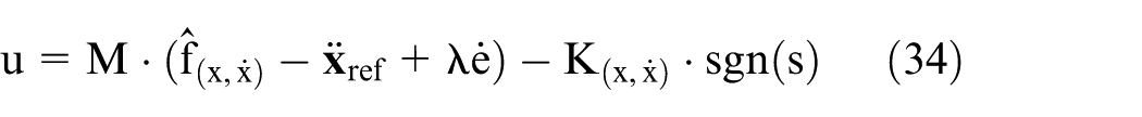
By choosing ${\mathrm{K}}_{(\mathrm{x},\stackrel{·}{\mathrm{x}})}$ to be large enough as $\mathrm{K}={\mathrm{F}}_{(\mathrm{x},\stackrel{·}{\mathrm{x}})}+\mathrm{\eta }$ , the final control input can be specified as equation (35), where $\mathrm{\lambda }=2220$ and $\mathrm{\eta }=2.5$ are strictly positive constants, which have been tuned and optimized to get the best response

$$\begin{array}{c}\multicolumn{1}{c}{\mathrm{u}=\mathrm{M}·(-{1.326310}^{-4}\stackrel{·}{\mathrm{x}}-{\stackrel{··}{\mathbf{x}}}_{\mathrm{ref}}+\lambda \stackrel{·}{\mathrm{e}}}\end{array})-(8.178\times {10}^{-5}\stackrel{·}{\mathrm{x}}+\mathrm{\eta })·\mathrm{sgn}(\stackrel{·}{\mathrm{e}}+\mathrm{\lambda }\mathrm{e})$$

(35)

Controller optimization

In order to optimize the controller parameters, the vertical speed must meet the step response requirements as rise time less than 0.3 s, settling time less than 1 s, and overshoot less than 1%. The controller variables to be optimized are separately as follows. Table 1 shows the current and optimized value of the variables for each controller:

• CPID; Proportional (P), Integral (I), Derivative (D), Filter Coefficient (N) of the inner loop (i), and outer loop (o);

• ADRC; Proportional (P), Derivative (D), Filter Coefficient (N), and Observer Bandwidth $({\omega }_0)$ ;

• LSC; Open-Loop Bandwidth $({\omega }_{\mathrm{c}})$ ;

• FEL1; Proportional (P), Derivative (D), and Filter Coefficient (N);

• FEL2; Proportional (P), Derivative (D), and Filter Coefficient (N);

• SMC; Positive Constants ( $\mathrm{\lambda }$ and $\mathrm{\eta }$ ).

Table 1.

Current value, bounds, and optimized value of the variables for each controller.

Controller	Variable name	Current value	Variable bounds		Scale	Optimized value
			Min	Max
CPID	${\mathrm{P}}_{\mathrm{o}}$	−667,795	−667,800	−667,700	2	−667,800
	${\mathrm{I}}_{\mathrm{o}}$	−85,473,222	−85,473,300	−85,473,200	2	−85,473,000
	${\mathrm{D}}_{\mathrm{o}}$	1074	−1100	−1050	1	−1074
	${\mathrm{N}}_{\mathrm{o}}$	2844	2800	2900	2	2844
	${\mathrm{P}}_{\mathrm{i}}$	107	100	150	1	126.13
	${\mathrm{I}}_{\mathrm{i}}$	641,860	641,800	641,900	2	641,800
	${\mathrm{D}}_{\mathrm{i}}$	−0.0014	−0.1	−0.001	0.01	−0.0018
	${\mathrm{N}}_{\mathrm{i}}$	23,788	23,700	23,800	2	23,788
ADRC	$\mathrm{P}$	−667	−700	−600	2	−670.306
	$\mathrm{D}$	−107	−150	−100	1	−150
	$\mathrm{N}$	2844	2800	2900	2	2850.4
	${\omega }_0$	48.4	10	300	1	155.6
LSC	${\omega }_{\mathrm{c}}$	800	200	1600	10	1400
FEL1	$\mathrm{P}$	−667,032,425	−667,032,500	−667,032,400	2	−667,032,425
	$\mathrm{D}$	0	−0.1	0	0.01	−0.000634
	$\mathrm{N}$	100	50	150	2	100
FEL2	$\mathrm{P}$	−667	−700	−600	2	−670.31
	$\mathrm{D}$	−107	−150	−100		−150
	$\mathrm{N}$	2844	2800	2900	2	2850.4
SMC	$\mathrm{\lambda }$	2500	2000	4000	200	3000
	$\mathrm{\eta }$	2.5	2	4	0.04	2.4998

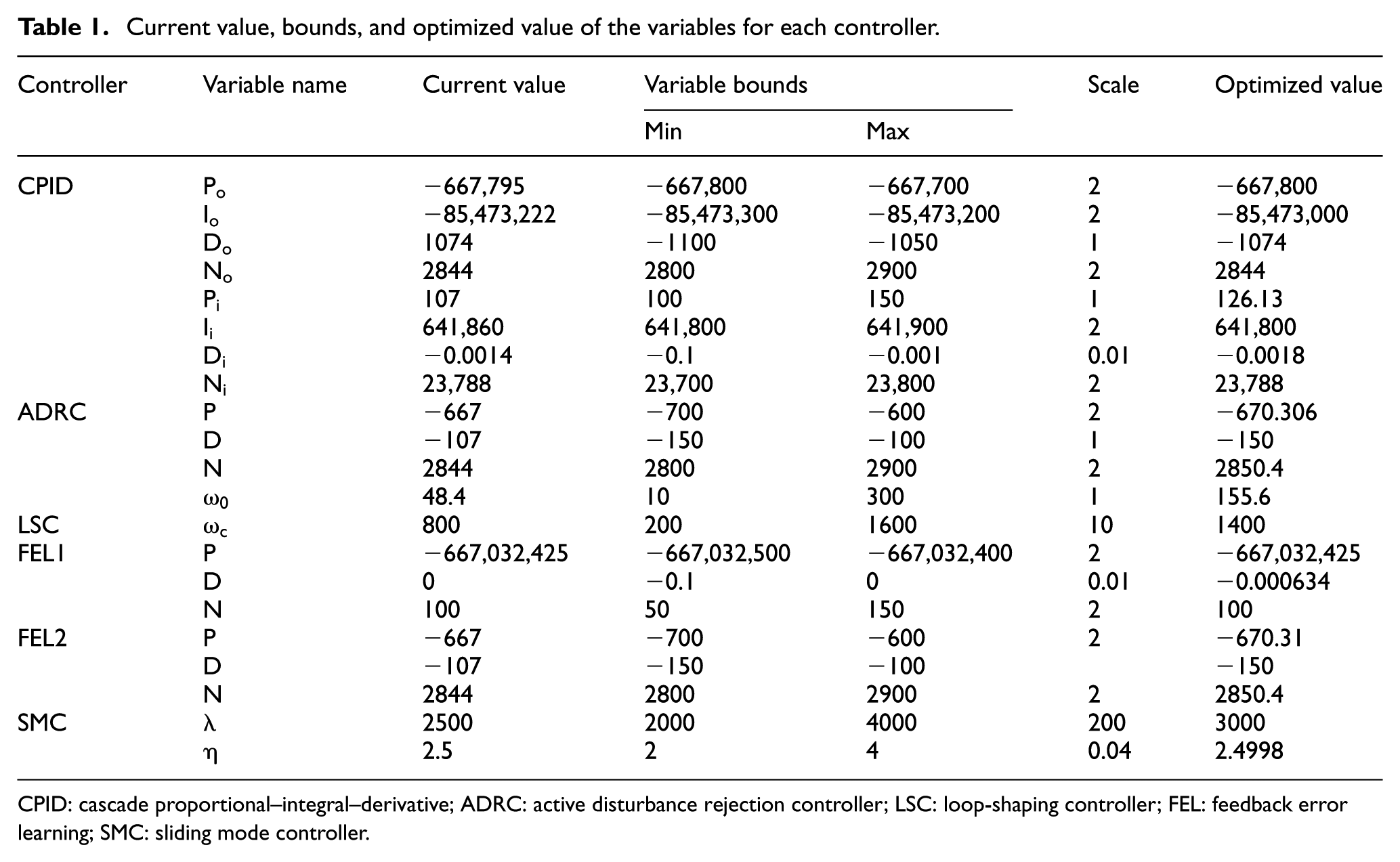
CPID: cascade proportional–integral–derivative; ADRC: active disturbance rejection controller; LSC: loop-shaping controller; FEL: feedback error learning; SMC: sliding mode controller.

Evaluation of the controllers

The evaluation and comparison of the designed controllers is implemented, using the performance measures described by equations (36)–(39). The integral square error (ISE), integral absolute error (IAE), integral of time weighted absolute error (ITAE), and root mean square error (RMSE) values are derived from the simulation results and then the performance of the controllers are evaluated. For vertical motion, the error signal is considered as $\mathrm{e}={\mathrm{\omega }}_{\mathrm{ref}}-\mathrm{\omega }$ , and for rotational motion as $\mathrm{e}={\omega }_{\mathrm{ref}}-\omega$

$$\mathrm{ISE}=\int {\mathrm{e}}^2·\mathrm{dt}$$

(36)

$$\mathrm{IAE}=\int \left|e\right|·\mathrm{dt}$$

(37)

$$\mathrm{ITAE}={\int }^{\mathrm{t}}·\left|e\right|·\mathrm{dt}$$

(38)

$$\mathrm{RMSE}=\sqrt{\int \frac{e^2}{\mathrm{n}}·\mathrm{dt}}$$

(39)

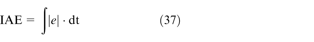
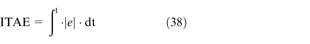
The ISE, which integrates the square of the error over time, is associated with the error energy. That means it penalizes the large errors more than the smaller ones. The IAE integrates the absolute error over time. It does not add weight to any of the errors in a systems response. In other words, the IAE reflexes the cumulative error, which means how far the response is with respect to the applied reference. The ITAE integrates the absolute error multiplied by the time over time. It can be meant, less importance to initial errors, whereas the present errors are much more considered.^48,49 The RMSE integrates the square of the error divided by the number of the samples over time. It represents appropriately the model performance, where the error distribution form is Gaussian. ⁵⁰ All of these integrals are evaluated over a fixed time period. It is infinity in theory, but will be enough until a time, when the responses are settled. It is worth mentioning that these measures are completely useless for measuring the performance of real control systems, but there are some other practical performance measures. The most frequently used one is the decay ratio as it gives a good indication of the stability of the controlled response. ⁴⁸

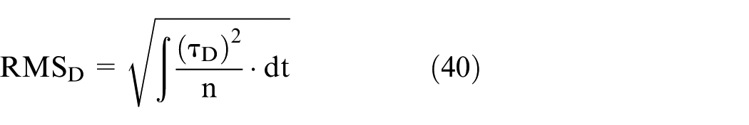
One more performance measure, which determines the energy consumption of each controller, is defined based on equation (40). In this equation “τ_D” is the torque input of the draw–works motor

$$\mathrm{RM}{\mathrm{S}}_{\mathrm{D}}=\sqrt{\int \frac{{\left({\tau }_{\mathrm{D}}\right)}^2}{\mathrm{n}}·\mathrm{dt}}$$

(40)

WOB controller

The optimization process of drilling parameters has direct effects on the cost reduction, which aims to optimize controllable variables during drilling operation such as WOB for obtaining maximum ROP, as the economic factor. ⁵¹ Determination of optimum WOB is very important in drilling operation as this parameter can be changed during drilling operation.

Based on the existing conditions and constraints in the field, during the drilling process the WOB parameter must be limited, in such a way not exceeding the determined value. To constrain the WOB limitation, three control architectures are designed. The first approach constrains the WOB limit by decreasing the vertical speed, the second one by increasing the rotational speed, and the last one combines these two approaches. In other words, it first increases the rotational speed to a certain limit and then decreases the vertical speed, in such a way the WOB limit is not exceeded. So long as the WOB is smaller than the determined value, the vertical and rotational speeds track their reference values, but once it exceeds the determined value, first the rotational speed reference increases, and then if it does not suffice, the vertical speed reference decreases by the WOB increase rate. As the vertical speed or ROP plays an economic role in the drilling process, our priority is increasing of rotational speed, instead of decreasing the ROP.

On the other hand, to provide a constant drilling state at the bit like WOB, and ROP, the autonomous drilling is generally implemented. The four individual modes of control for autonomous drilling are WOB mode, ROP mode, Delta–P mode, and Torque mode. In the WOB mode, the control system controls the vertical speed or ROP to maintain a preset constant WOB, which is the optimum value of it. The optimization methods can be applied to the problem of selecting the best WOB to achieve the minimum cost per foot. ⁴⁵ To design such a controller, two different architectures can be implemented. In the first approach, based on equation (3), which represents the WOB according to the vertical and rotational speed, we can derive the proper vertical speed reference to give a predetermined value for the WOB, assuming a constant rotational speed. By this approach, it is assumed that the rock stiffness is determined or it can be estimated by a special observer. In the second approach, the proper vertical speed reference can be easily achieved by the production of the measured vertical speed and the difference rate of measured and predetermined WOB.

Test and results

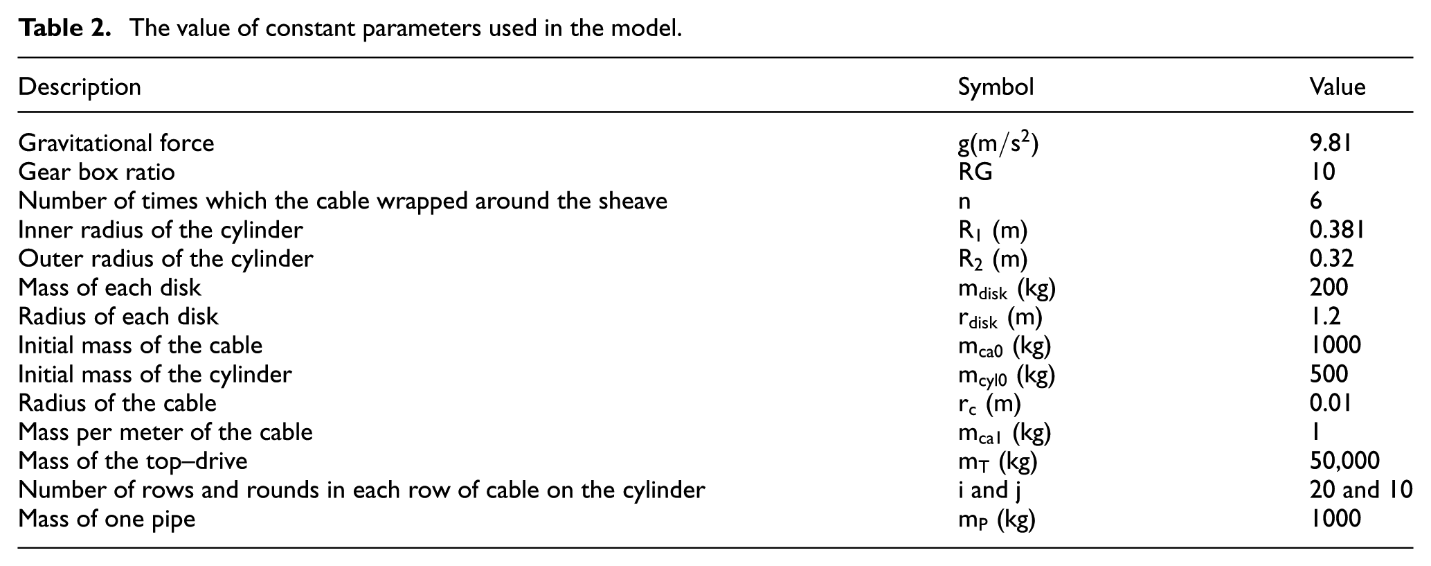
Table 2 demonstrates the value of the constant parameters which have been used in the simulation model.

Table 2.

The value of constant parameters used in the model.

Description	Symbol	Value
Gravitational force	$\mathrm{g}(\mathrm{m}/{\mathrm{s}}^2)$	9.81
Gear box ratio	$\mathrm{RG}$	10
Number of times which the cable wrapped around the sheave	$\mathrm{n}$	6
Inner radius of the cylinder	${\mathrm{R}}_1(\mathrm{m})$	0.381
Outer radius of the cylinder	${\mathrm{R}}_2(\mathrm{m})$	0.32
Mass of each disk	${\mathrm{m}}_{\mathrm{disk}}(\mathrm{kg})$	200
Radius of each disk	${\mathrm{r}}_{\mathrm{disk}}(\mathrm{m})$	1.2
Initial mass of the cable	${\mathrm{m}}_{\mathrm{ca}0}(\mathrm{kg})$	1000
Initial mass of the cylinder	${\mathrm{m}}_{\mathrm{cyl}0}(\mathrm{kg})$	500
Radius of the cable	${\mathrm{r}}_{\mathrm{c}}(\mathrm{m})$	0.01
Mass per meter of the cable	${\mathrm{m}}_{\mathrm{ca}1}(\mathrm{kg})$	1
Mass of the top–drive	${\mathrm{m}}_{\mathrm{T}}(\mathrm{kg})$	50,000
Number of rows and rounds in each row of cable on the cylinder	$\mathrm{i}\mathrm{and}\mathrm{j}$	20 and 10
Mass of one pipe	${\mathrm{m}}_{\mathrm{P}}(\mathrm{kg})$	1000

The disturbance signals as a part of the uncertain forces, which are applied on the vertical and rotational motions during the tripping and drilling operations, are displayed in Figure 10. It is worth mentioning that they are roughly 10 times larger than the applied torques by the controller on the draw–works and top–drive, respectively.

Figure 10.

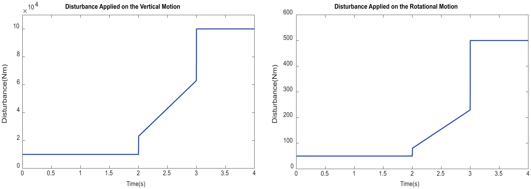
Disturbance signals, applied on the vertical and rotational motions during the tripping and drilling operations.

First, the performance of the controllers during tripping operation for vertical motion is evaluated. The reference and hook vertical speeds using each controller are demonstrated in Figure 11. As a visual result, we can conclude that all of the designed controllers can track well the given references and reject the effect of the applied disturbance on the vertical dynamic successfully. Table 3 shows the performance measures of each controller separately.

Figure 11.

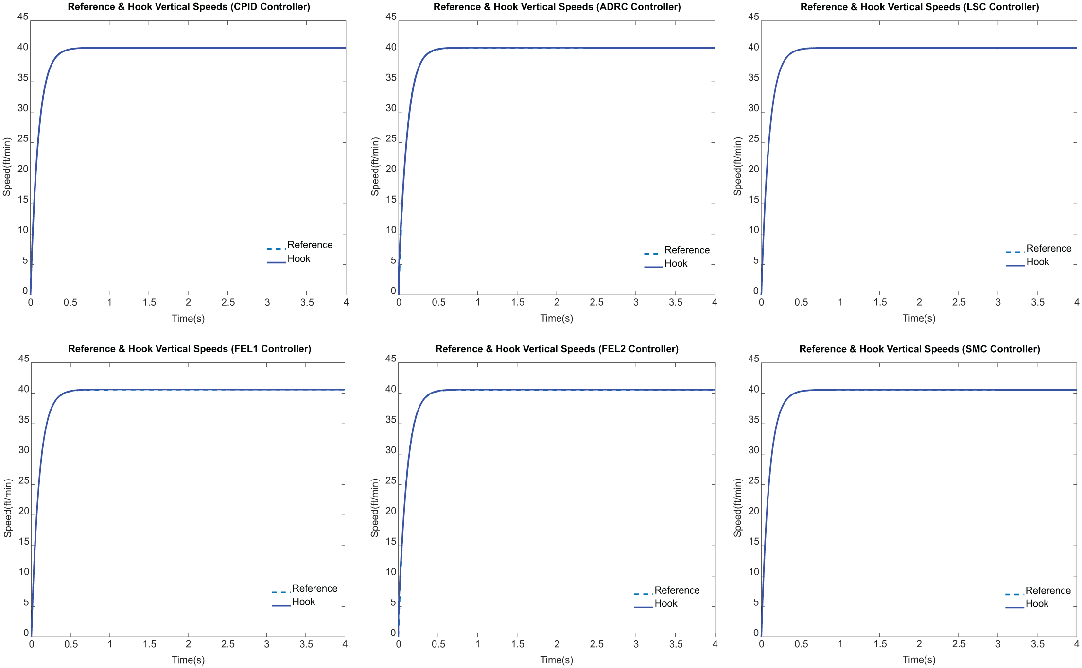
Reference and hook vertical speeds of each controller during tripping operation.

Table 3.

Performance measures of each controller during tripping operation.

Controller	Performance measure
	ISE	IAE	ITAE	RMSE
CPID	0.0153	0.8642	0.0509	0.0043
ADRC	23680	14385	953.75	71.92
LSC	0.2177	20.2837	1.1524	0.1014
FEL1	0.3749	87.8863	11.525	0.4394
FEL2	23675	14382	953.5	71.9
SMC	639.01	3481.5	317.99	17.40

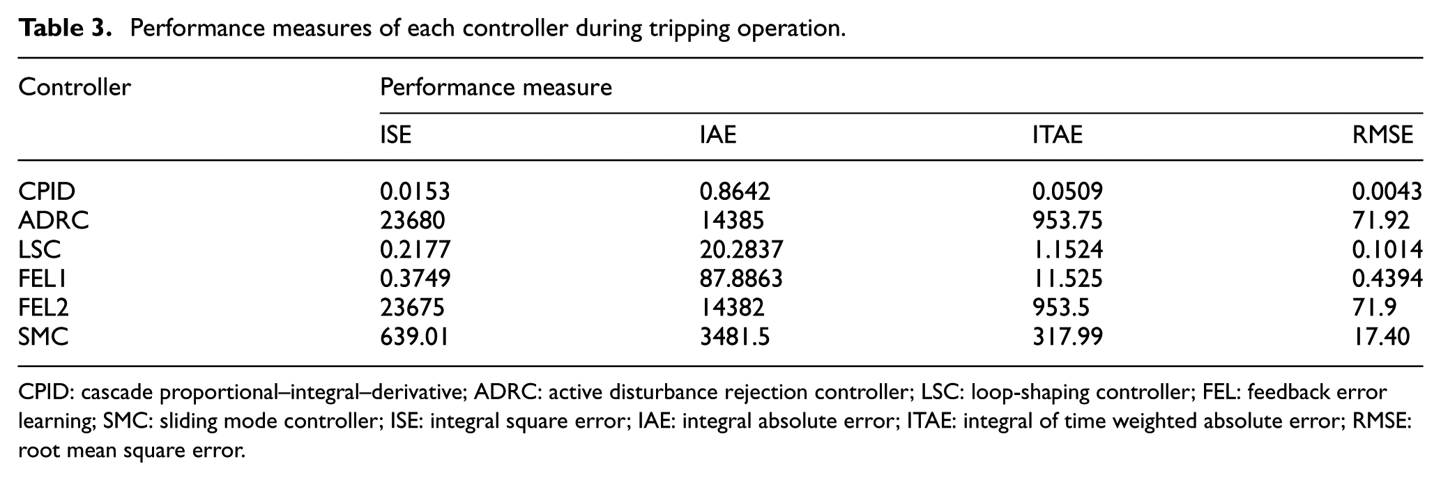
CPID: cascade proportional–integral–derivative; ADRC: active disturbance rejection controller; LSC: loop-shaping controller; FEL: feedback error learning; SMC: sliding mode controller; ISE: integral square error; IAE: integral absolute error; ITAE: integral of time weighted absolute error; RMSE: root mean square error.

As it can be derived from Table 3, the minimum ISE belongs to CPID controller, while the ADRC has the maximum value. This means CPID controller has the minimum and ADRC the maximum error energy, or it can be said, CPID has the minimum amount of large errors, and ADRC has the maximum amount of large errors among the other controllers. Similarly, the minimum cumulative error IAE belongs to CPID controller, while the ADRC has the maximum cumulative error. It can be concluded that the CPID controller gives the nearest response and the ADRC gives the furthest response with respect to the applied reference. From the ITAE values, it can be seen that the minimum steady–state error is for CPID controller and the maximum one for ADRC. Or it can be said, the system response by CPID settles much more quickly than the other controllers. The same result can be concluded from the RMSE values.

Table 4 demonstrates the energy consumption of the controllers, and as it is seen, the LSC controller consumes the minimum and SMC the maximum energy.

Table 4.

Energy consumption of each controller during tripping operation.

Controller	$\mathrm{RM}{\mathrm{S}}_{\mathrm{D}}$
CPID	17.272e05
ADRC	6.2312e05
LSC	1.4963e05
FEL1	1.4964e05
FEL2	5.1314e05
SMC	1.831e07

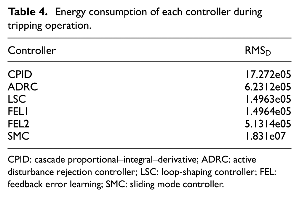
CPID: cascade proportional–integral–derivative; ADRC: active disturbance rejection controller; LSC: loop-shaping controller; FEL: feedback error learning; SMC: sliding mode controller.

Second, the performance of the controllers during drilling operation for both vertical and rotational motions is evaluated. As mentioned previously, drilling action comprises the vertical penetration of the drill bit and the rotational motion of the drill–string. The design of control process for all five types of controllers are similarly implemented to rotational motion dynamics as presented in equation (2).

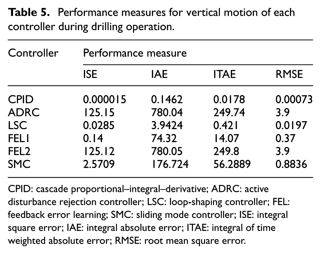
The reference and hook vertical speeds using each controller are demonstrated in Figure 12. Table 5 shows the performance measures of each controller. It is worth mentioning that the rock stiffness has been constructed and applied to the system as a time signal represented in Figure 13, which causes a changing WOB. As a visual result from the figures, we can conclude that all of the designed controllers can track well the given references and reject the effect of the applied disturbance on the vertical dynamic successfully.

Figure 12.

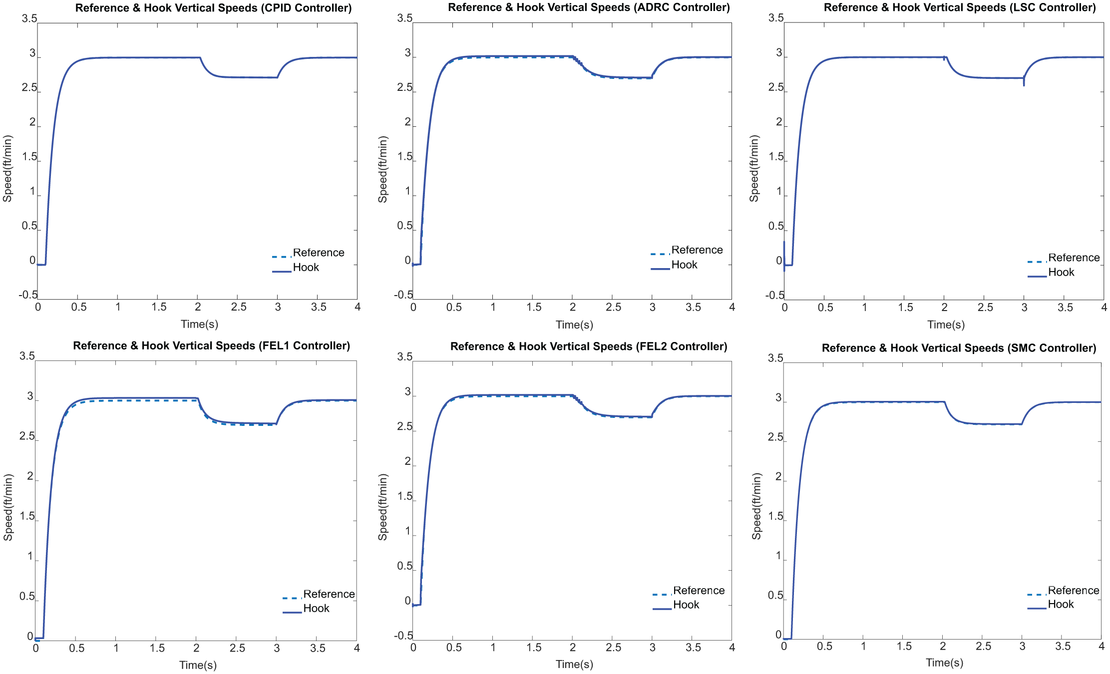
Reference and hook vertical speeds of each controller during drilling operation.

Table 5.

Performance measures for vertical motion of each controller during drilling operation.

Controller	Performance measure
	ISE	IAE	ITAE	RMSE
CPID	0.000015	0.1462	0.0178	0.00073
ADRC	125.15	780.04	249.74	3.9
LSC	0.0285	3.9424	0.421	0.0197
FEL1	0.14	74.32	14.07	0.37
FEL2	125.12	780.05	249.8	3.9
SMC	2.5709	176.724	56.2889	0.8836

CPID: cascade proportional–integral–derivative; ADRC: active disturbance rejection controller; LSC: loop-shaping controller; FEL: feedback error learning; SMC: sliding mode controller; ISE: integral square error; IAE: integral absolute error; ITAE: integral of time weighted absolute error; RMSE: root mean square error.

Figure 13.

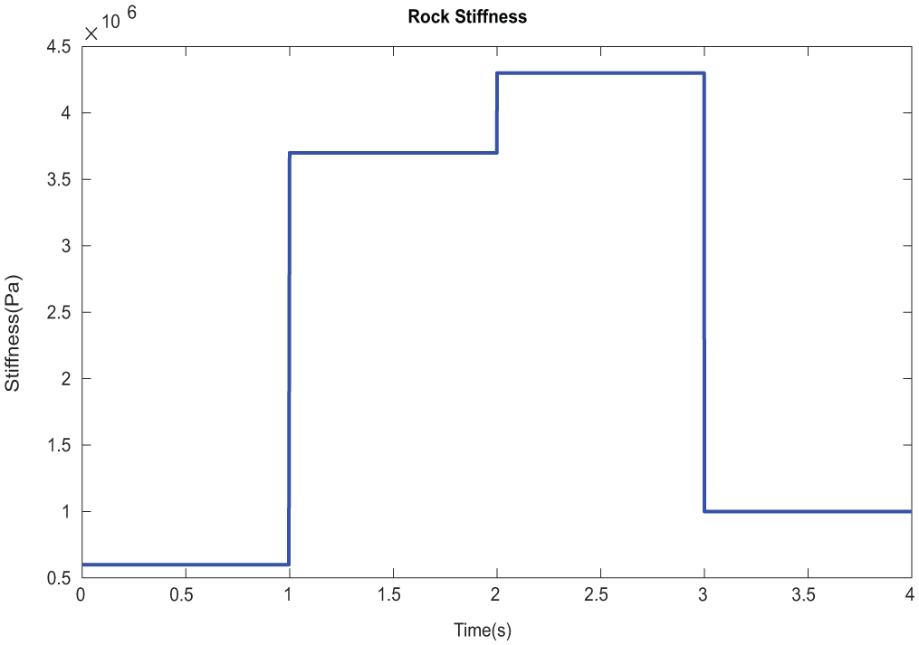
Rock stiffness time signal.

For vertical motion, during drilling process, the minimum ISE, IAE, ITAE, and RMSE belongs to CPID controller, while the maximum ISE to the ADRC, maximum IAE and ITAE to FEL2, and roughly same maximum RMSE to ADRC and FEL2. From these points, it can be concluded that CPID controller has the minimum error energy, gives the nearest response with respect to the applied reference, and has the minimum steady–state error. On the other hand, ADRC has the maximum error energy, while FEL2 gives the furthest response with respect to the applied reference and has the maximum steady–state error.

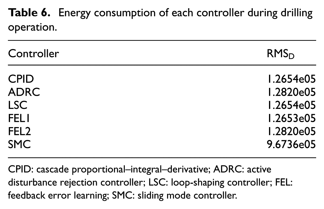
Table 6 demonstrates the energy consumption of the controllers, and as it is seen, the FEL1 controller consumes the minimum and SMC the maximum energy.

Table 6.

Energy consumption of each controller during drilling operation.

Controller	$\mathrm{RM}{\mathrm{S}}_{\mathrm{D}}$
CPID	1.2654e05
ADRC	1.2820e05
LSC	1.2654e05
FEL1	1.2653e05
FEL2	1.2820e05
SMC	9.6736e05

CPID: cascade proportional–integral–derivative; ADRC: active disturbance rejection controller; LSC: loop-shaping controller; FEL: feedback error learning; SMC: sliding mode controller.

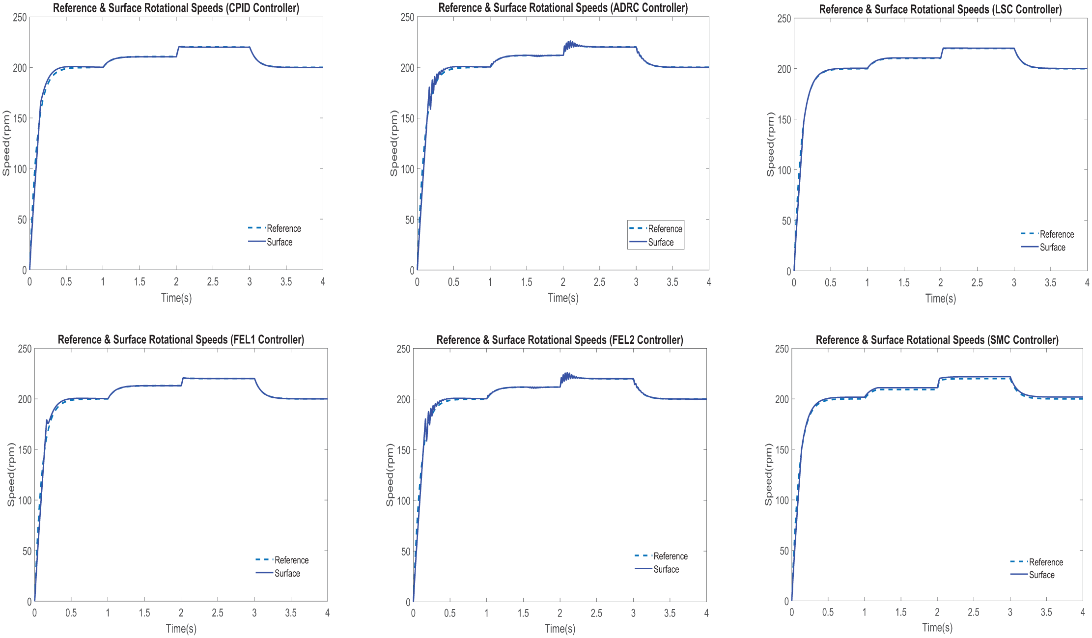
The reference and surface rotational speeds using each designed controller are demonstrated in Figure 14. As a visual result, we can conclude that all of the designed controllers can track well the given references and reject the effect of the applied disturbance on the rotational dynamic successfully. Table 7 shows the performance measures of each controller.

Figure 14.

Reference and surface rotational speeds of each controller during drilling operation.

Table 7.

Performance measures for rotational motion of each controller during drilling operation.

Controller	Performance measure
	ISE	IAE	ITAE	RMSE
CPID	197.09	2665.3	526.5	13.33
ADRC	957.6	5180.9	868.98	25.9
LSC	369.7	3619.9	852.8	18.1
FEL1	388.32	3797.1	732.9	18.9
FEL2	959.87	5184.0	868.50	25.92
SMC	2732.3	8363.8	2391.9	41.82

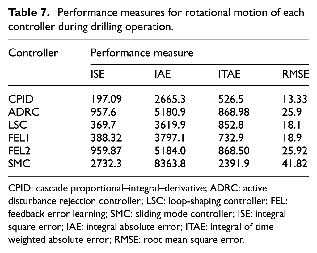
CPID: cascade proportional–integral–derivative; ADRC: active disturbance rejection controller; LSC: loop-shaping controller; FEL: feedback error learning; SMC: sliding mode controller; ISE: integral square error; IAE: integral absolute error; ITAE: integral of time weighted absolute error; RMSE: root mean square error.

For rotational motion, during drilling process, the minimum ISE, IAE, ITAE, and RMSE belongs to CPID controller, while the maximum values to the SMC controller. From these points, it can be concluded that CPID controller has the minimum error energy, gives the nearest response with respect to the applied reference, and has the minimum steady–state error, while SMC has the maximum error energy, gives the furthest response with respect to the applied reference, and has the maximum steady–state error.

Third, in order to evaluate the behavior of the WOB limiter during drilling process using three mentioned architectures, the following results are presented. Figures 15–17 demonstrate the vertical and rotational speeds and the limited WOB using the first, second, and third approaches, respectively.

Figure 15.

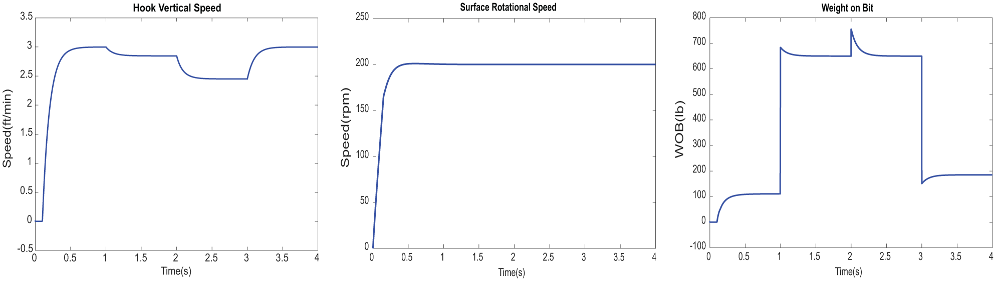
Vertical and rotational speeds and weight on bit using the first approach.

Figure 16.

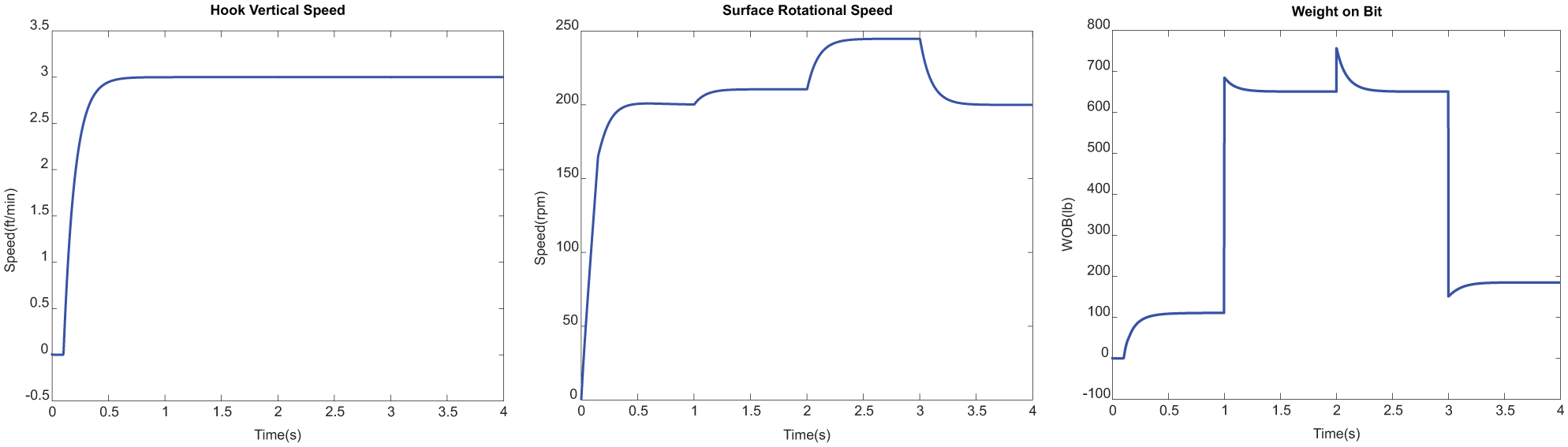
Vertical and rotational speeds and weight on bit using the second approach.

Figure 17.

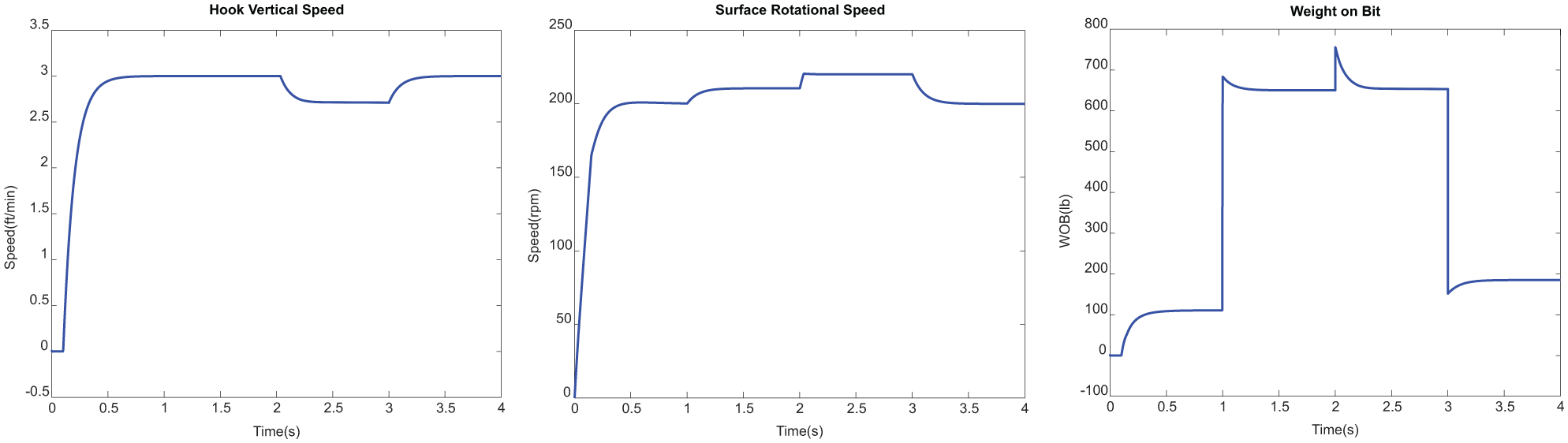
Vertical and rotational speeds and weight on bit using the third approach.

As it can be seen from Figures 15–17, to limit the WOB level at 650 lb, as a realistic constraint, in the first approach just the vertical speed decreases, in the second approach just the rotational speed increases, and in the third approach both of them change, which means first the rotational speed increases to a determined value (220 r/min), and because it does not suffice, the vertical speed decreases. The results show the good performance of all three proposed control approaches.

Finally, the behavior of the autonomous drilling in WOB mode is evaluated using the two designed control architectures. Figures 18 and 19 demonstrate the vertical speed and the WOB using two approaches, respectively. In the first approach, it is assumed that the rock stiffness is determined as presented in Figure 13. In real plant, the rock stiffness can be estimated by a properly designed observer.

Figure 18.

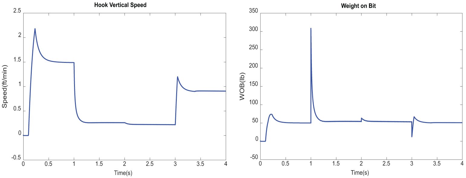
Vertical speed and weight on bit using the first approach.

Figure 19.

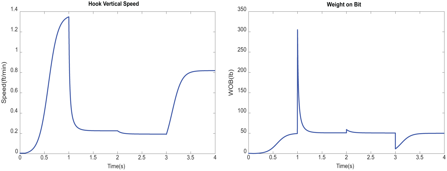
Vertical speed and weight on bit using the second approach.

As it can be seen from the above presented figures, a constant WOB 50 lb, as an optimum WOB, is successfully maintained using both of the approaches. In both of them, the vertical speed is properly changing according to the rock stiffness.

Conclusion

In this paper, we presented design process of five types of robust and/or adaptive control systems for a drilling rig during operating modes in detail. The performances of designed CPID, active disturbance rejection, loop shaping, FEL, and SMCs during tripping and drilling processes were studied, and their performance measures and also energy consumptions were evaluated. The effects of the uncertain forces including the structured or parametric model uncertainties and the applied external disturbances on the system were successfully eliminated using the ability of the designed adaptive and/or robust controllers. In addition, to control the WOB during drilling process, some proper architectures were presented.

Generally, the CPID controller had the best performance in both of the tripping and drilling operations. From the point of view of energy consumption, the LSC was the best one in the tripping operation and the FEL1 controller in the drilling operation. Three presented control approaches to limit the weight on bit, and also two approaches to maintain a preset constant weight on bit, behave as well as expected. Overall, the simulation results showed the good performance of all proposed control architectures.