A continuous integral terminal sliding mode control approach for a class of uncertain nonlinear systems

Abstract

In this article, the continuous integral terminal sliding mode control problem for a class of uncertain nonlinear systems is investigated. First of all, based on homogeneous system theory, a global finite-time control law with simple structure is proposed for a chain of integrators. Then, inspired by the proposed finite-time control law, a novel integral terminal sliding mode surface is designed, based on which an integral terminal sliding mode control law is constructed for a class of higher order nonlinear systems subject disturbances. Furthermore, a finite-time disturbance observer-based integral terminal sliding mode control law is proposed, and strict theoretical analysis shows that the composite integral terminal sliding mode control approach can eliminate chattering completely without losing disturbance attenuation ability and performance robustness of integral terminal sliding mode control. Simulation examples are given to illustrate the simplicity of the new design approach and effectiveness.

Introduction

Sliding mode control (SMC) is a nonlinear control strategy, which usually demonstrates fine robust properties with respect to parameter uncertainties and disturbances. ¹ SMC has been widely used in many practical systems such as robotic systems, ² spacecraft systems, ³ maglev suspension systems, ⁴ mechanical systems, ⁵ and piezoelectric-driven motion system.^6,7 The conventional SMC methods could render the linear sliding mode manifold be reached in finite time.

Different to SMC scheme, a nonlinear sliding mode manifold is employed in nonsingular terminal sliding mode control (NTSMC),^8,9 which makes that NTSMC not only keeps the main advantages of conventional SMC but also can guarantee that the states trajectories converge to the equilibrium in finite time. Compared to asymptotical stability, besides faster convergence rate, the closed-loop systems under finite-time control (FTC) law usually demonstrate higher accuracy and better disturbance rejection properties. ¹⁰ In view of these advantages, FTC problems have received a lot of attention recently.^11–34 Due to the superior properties of NTSMC, NTSMC has attracted significant interests from the control field.^{8,9,16,35–37} Recently, based on Bhat and Bernstein, ¹¹ NTSMC is developed to a class of higher order nonlinear systems.^38,39 Despite NTSMC possesses significant theoretical and practical values, the study of NTSMC for higher order nonlinear systems is still quite underdeveloped, and further research is needed.

This article is devoted to develop a novel NTSMC approach, that is, an integral terminal sliding mode control (ITSMC) approach, for a class of higher order nonlinear systems. More specifically, inspired by Bhat and Bernstein ¹¹ and Qian and Li ²¹ and the ITSMC approach in Xu, ⁴⁰ a novel global FTC law is proposed for a chain of integrators based on weighted homogeneity theory^41,42 first. Then, based on the proposed FTC law, a novel ITSMC approach is introduced for a class of higher order nonlinear systems subject disturbances (hereafter the disturbances may include parameter uncertainties and external disturbances). Note that the discontinuity of the proposed ITSMC may lead to significant chattering. Although adaptive control has some robust ability and will not bring chattering, it is often ineffective when the considered system subject to strong disturbances^43–51 is designed to estimate the disturbances; then a continuous composite ITSMC control law is proposed for the considered nonlinear systems. Within our methodology, it is easy to tune the control law parameters for the desired performances; thus, it is more suitable for practical applications. Simulation examples are carried out to show the validation of the proposed methods.

The outline of this article is as follows. In the “Preliminaries” section, preliminaries are given. The “Main results” section displays the control strategies for higher order nonlinear systems. Finally, concluding remarks are given in the “Conclusion” section.

Notations

Throughout this article, $\mathbb{R}$ and ${\mathbb{R}}^n$ denote real numbers and n-dimensional Euclidean space, respectively. A function $f(·)\in {\mathbb{C}}^k$ represents that $f(·)$ is $k-\mathrm{times}$ continuously differentiable on its domain, and $[·{]}^k=|·{|}^k\mathrm{sign}(·)$ . Let $\mathcal{A}$ be a set, $\partial \mathcal{A}$ denote the boundary of $\mathcal{A}$ .

Preliminaries

In this section, we will introduce several useful lemmas, which will be used throughout the article.

Definition 2.1

Weighted homogeneity: For fixed coordinates $(x_1,\dots ,x_n{)}^T\in {\mathbb{R}}^n$ and real numbers $r_i>0,i=1,\dots ,n$ , (a) the dilation ${\Delta }_{\epsilon }(x)=({\epsilon }^{r_1}{x}_1,\dots ,{\epsilon }^{r_n}{x}_n),\forall \epsilon >0$ , with $r_i$ being called as the weights of the coordinates (for simplicity of notation, we define dilation weight $\Delta =(r_1,\dots ,r_n)$ ); (b) a function $V\in \mathbb{C}({\mathbb{R}}^n,\mathbb{R})$ is said to be homogeneous of degree $\tau$ if there is a real number $\tau \in \mathbb{R}$ such that $\forall x\in \mathbb{R}\backslash \{0\},\epsilon >0,V({\Delta }_{\epsilon }(x))={\epsilon }^{\tau }V(x_1,\dots ,x_n)$ ; (c) a vector field $f\in \mathbb{C}({\mathbb{R}}^n,{\mathbb{R}}^n)$ is said to be homogeneous of degree $\tau$ if there is a real number $\tau \in \mathbb{R}$ such that for $i=1,\dots ,n$ , $\forall x\in \mathbb{R}\backslash \{0\},{\epsilon }_i>0,f_i({\Delta }_{\epsilon }(x))={\epsilon }^{\tau +r_i}{f}_i(x_1,\dots ,x_n)$ .^21,42,52

Lemma 2.1

Given the trivial solution $x=0$ of system $\stackrel{·}{x}=f(x)$ is asymptotically stable, and $f(x)$ is continuous and homogeneous of degree $\alpha$ with respect to dilation weight $(r_1,\dots ,r_n)$ . ⁴¹ Then for any positive integer $p$ and any $\sigma >p\times \{r_1,\cdots ,r_n\}$ , there exists a ${\mathbb{C}}^p$ homogeneous Lyapunov function $V(x)$ of degree $\sigma$ with respect to $(r_1,\cdots ,r_n{)}^T$ , such that $\stackrel{·}{V}(x)\le -c{V}^{(\sigma +\alpha )/\sigma }(x)$ with $c>0$ .

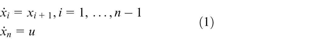
Consider the following chain of integrators

$$\begin{array}{c}{\stackrel{·}{x}}_i=x_{i+1},i=1,\dots ,n-1\hfill \\ {\stackrel{·}{x}}_n=u\hfill \end{array}$$

(1)

where $x=(x_1,\dots ,x_n{)}^T\in {\mathbb{R}}^n$ and $u\in \mathbb{R}$ are the system state and control input, respectively.

For system (1), based on weighted homogeneity theory ⁴² and the adding a power integrator technique, ⁵³ Qian and Li ²¹ proposed an FTC method, while Bhat and Bernstein ¹¹ considered FTC design method for system (1) based on geometric homogeneity theory, which can be described by the following two lemmas, respectively.

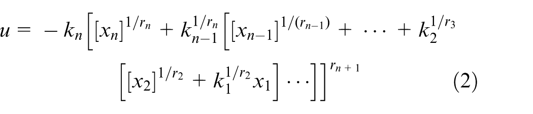
Lemma 2.2

For any constant $\tau \in (-(1/n),0)$ , there exists a homogeneous state feedback control law with the form ²¹

$$u=-k_n[{\left[x_n\right]}^{1/r_n}+k_{n-1}^{1/r_n}[{\left[x_{n-1}\right]}^{1/(r_{n-1})}+\cdots +k_2^{1/r_3}{[{\left[x_2\right]}^{1/r_2}+k_1^{1/r_2}{x}_1]\cdots ]]}^{r_{n+1}}$$

(2)

where $k_i>0,i=1,\dots ,n$ are constants, and

$$r_1=1,r_i=r_1+(i-1)\tau ,i=1,\dots ,n+1$$

(3)

such that the closed-loop systems (1) and (2) are globally finite-time stable.

Remark 2.1

It should be pointed out that due to the nature of adding a power integrator technique, in Lemma 2.2, the control parameters $k_i\mathrm{s}$ may increase significantly along with the system dimension. Under the control law (2), it is clear that the closed-loop systems (1) and (2) are homogeneous of degree $\tau$ with respect to dilation weights $(r_1,\dots ,r_n)$ .

Lemma 2.3

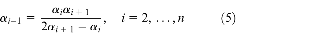
Let $k_1,\cdots ,k_n>0$ be such that the polynomial $s^n+k_n{s}^{n-1}+\cdots +k_{2}s+k_1$ is Hurwitz, then there exists $\epsilon \in (0,1)$ such that, for every $\alpha \in (1-\epsilon ,1)$ , the origin is a globally finite-time stable equilibrium for the system (1) under the feedback control law ¹¹

$$u=-k_1{\left[x_1\right]}^{{\alpha }_1}-\cdots -k_n{\left[x_n\right]}^{{\alpha }_n}$$

(4)

where ${\alpha }_1,\dots ,{\alpha }_n$ satisfy

$${\alpha }_{i-1}=\frac{{\alpha }_i{\alpha }_{i+1}}{2{\alpha }_{i+1}-{\alpha }_i},i=2,\dots ,n$$

(5)

with ${\alpha }_{n+1}=1$ and ${\alpha }_n=\alpha$ .

Remark 2.2

Lemma 2.3 is obtained based on geometric homogeneity theory. Compared to Lemma 2.2, it is easy to choose control parameter $k_i$ , $i=1,\dots ,n$ , for control law (4).

Lemma 2.4

Let $\mathcal{X}$ and $\mathcal{Y}$ be topological spaces with $\mathcal{Y}$ compact and consider the product space $\mathcal{X}\times \mathcal{Y}$ . If $\mathcal{Z}$ is an open set of $\mathcal{X}\times \mathcal{Y}$ containing the slice ${\tau }_0\times \mathcal{Y}$ of $\mathcal{X}\times \mathcal{Y}$ , then $\mathcal{Z}$ contains some tube $\mathcal{W}\times \mathcal{Y}$ about ${\tau }_0\times \mathcal{Y}$ , where $\mathcal{W}$ is a neighborhood of ${\tau }_0$ in $\mathcal{X}$ .^54,55

Inspired by Lemmas 2.2 and 2.3, we have the following result for system (1) based on weighted homogeneity theory, Lemmas 2.1 and 2.4, which will be a key role for the main results of this article.

Theorem 1

There exists $\tau \in (-(1/n),0)$ such that the system (1) can be globally stabilized in finite time under the homogeneous control law

$$u=-k_1{\left[x_1\right]}^{r_{n+1}/r_1}-\cdots -k_n{\left[x_n\right]}^{r_{n+1}/r_n}$$

(6)

where $k_1,\dots ,k_n>0$ are the coefficients of Hurwitz polynomial $s^n+k_n{s}^{n-1}+\cdots +k_{2}s+k_1$ , and $r_i$ , $i=1,\dots ,n+1$ , is defined in equation (3).

Proof

For each $\tau \in (-(1/n),0)$ , the closed-loop systems (1) and (6) can be described by the following compact form

$$\stackrel{·}{x}=f_{\tau }\left(x\right)$$

(7)

where $f_{\tau }(·)=(f_{\tau 1}(·),f_{\tau 2}(·),\dots ,f_{\tau n}(·){)}^T$ denotes the right-hand side continuous vector functions of the closed-loop system. It is easy to show that system (7) is homogeneous with degree $\tau$ with respect to dilation weights $(r_1,\dots ,r_n)$ .

As $\tau =0$ , system (7), that is, $\stackrel{·}{x}=f_0(x)$ , is a linear system with the Hurwitz characteristic polynomial $s^n+k_n{s}^{n-1}+\cdots +k_{2}s+k_1$ . According to Lemma 2.1, there exists a positive definite, radially unbounded homogeneous Lyapunov function $V:{\mathbb{R}}^n\to \mathbb{R}$ such that $\stackrel{·}{V}=\sum _{i=1}^n(\partial V/\partial x_i)f_{0i}(x)$ is continuous and negative definite.

Let $\Omega =V^{-1}([0,1])$ and $\Lambda =\partial \Omega =V^{-1}(\{1\})$ . Then both $\Omega$ and $\Lambda$ are compact sets. Define $\eta :(-1,0]\times \Lambda \to \mathbb{R}$ by $\eta (\tau ,x)=\sum _i^n(\partial V/\partial x_i)f_{\tau i}(x)$ , then $\eta (·)$ is a continuous function and satisfies $\eta (0,x)<0$ for all $x\in \Lambda$ , that is, $\eta (\{0\}\times \Lambda )\subset (-\infty ,0)$ . Note that $\Lambda$ is compact and $\eta (·)$ is continuous; according Lemma 2.4, there exists a $\delta >0$ such that $\eta ((-\delta ,0]\times \Lambda )\subset (-\infty ,0)$ . Let $ϵ=\min \{\delta ,(1/n)\}$ , it follows that for $\tau \in (-ϵ,0)$ , $\eta (\tau ,x)$ is negative on $\Lambda$ . Therefore, $\Omega$ is strictly positively invariant under $f_{\tau }(·)$ for every $\tau \in (-ϵ,0]$ , and system (7) is globally asymptotically stable.

As $\tau \in (-ϵ,0)$ , system (7) is homogeneous of degree $\tau <0$ ; it follows that system (7) is globally finite-time stable.

Remark 2.3

Compared to Lemma 2.2, the advantage of Theorem 1 lies in the following aspects: (a) the structure of the control law (6) is more simpler than that of (2), and (b) it is easier to choose control law parameters. Similar to Lemma 2.3, in Theorem 1, we proved that the control law (6) will steer the states of system (1) to the origin in finite time based on geometric homogeneity. ¹¹ It is easy to obtain a homogeneous Lyapunov inequality, that is, the positive constant $c$ in $\stackrel{·}{V}(x)\le -c{V}^{(\sigma +\alpha )/\sigma }(x)$ is dependent on homogeneous degree. ³² Therefore, the disadvantage of Theorem 1 is that one could not provide the convergence time precisely.

Compared to Lemma 2.3, Theorem 1 has the following merits. (a) It is easier to choose parameters for control law (6). Specifically, once $k_i,i=1,\dots ,n$ are chosen, one only needs to care about how to choose an appropriate parameter $\tau$ by Theorem 1. However there are two parameters need to choose according to Lemma 2.3, that is, one needs to care about how to choose $\epsilon$ and $\alpha$ in Lemma 2.3. (b) In equation (3), once $\tau$ is chosen, it is easier to calculate the power of the control law (6), while according to equation (5), it is more complex to calculate ${\alpha }_i\mathrm{s}$ with the increase of the dimension of system (1). (c) Both equations (4) and (6) are homogeneous control laws for system (1); it is clear that the closed-loop systems (1) and (6) are homogeneous of degree $\tau$ with respect to dilation weights $(r_1,\dots ,r_n)$ , while it is not easy to calculate the homogeneous degree and the dilation of the closed-loop systems (1) and (4) with the increase of dimension of system (1).

The effectiveness of the propose control scheme can be shown by the following numerical example.

Example 1

Consider the following triple integrator system for simulation studies

$${\stackrel{·}{x}}_1=x_2,{\stackrel{·}{x}}_2=x_3,{\stackrel{·}{x}}_3=u$$

(8)

For comparison studies, both Lemma 2.3 and Theorem 1 are employed in the simulation. According to Lemma 2.3 and Theorem 1, we can design the following two control laws

$$u=-k_1{\left[x_1\right]}^{{\alpha }_1}-k_2{\left[x_2\right]}^{{\alpha }_2}-k_3{\left[x_3\right]}^{{\alpha }_3}$$

(9)

$$u=-k_1{\left[x_1\right]}^{r_4/r_1}-k_2{\left[x_2\right]}^{r_4/r_2}-k_3{\left[x_3\right]}^{r_4/r_3}$$

(10)

for system (8), respectively.

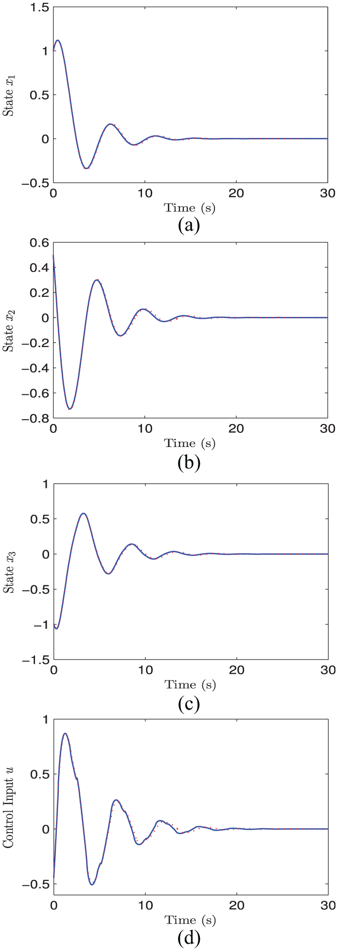
To have a fair comparison, we choose the same control gains $k_1=0.8,k_2=1.5,k_3=1.2$ for control laws (9) and (10). Furthermore, according to Bhat and Bernstein, ¹¹ under control law (9), the closed-loop systems (8) and (9) are homogeneous of degree $(\alpha -1)/\alpha$ . Here, we choose $\alpha =25/27$ and $\tau =-2/25$ such that the closed-loop system is homogeneous of degree $-2/25$ under two different control laws (9) and (10). According to Lemma 2.3 and Theorem 1, we obtain that ${\alpha }_1=25/31,{\alpha }_2=25/29,{\alpha }_3=25/27$ and $r_2=23/25,r_3=21/25,r_4=19/25$ . The simulation is conducted with $(x_1(0),x_2(0),x_3(0))=(1,0.5,-1)$ . The response curves of the system (8) under the two different control schemes are shown in Figure 1. It can be observed from Figure 1 that both of the two control laws (9) and (10) can stabilize system (8) rapidly.

Figure 1.

Responses of system (8) under control laws (9) (the dotted line) and (10) (the solid line). (a) The response curve of the state $x_1$ ; (b) The response curve of the state $x_2$ ; (c) The response curve of the state $x_3$ ; (d) The response curves of the two input signals.

Remark 2.4

In order to guarantee that $r_i>0,i=1,\dots ,n+1$ , Lemma 2.2 and Theorem 2 demand that $\tau \in (-(1/n),0)$ , and under the control law (6), the closed-loop system is homogeneous of degree $\tau$ . According to Bhat and Bernstein, ¹¹ under the control law (4), the closed-loop system is homogeneous of degree with $(\alpha -1)/\alpha$ . For the same system (1), if $-(1/n)=\tau =(\alpha -1)/\alpha$ , then we have $\alpha =n/(n+1)$ . Therefore, according to Lemma 2.3, if one choose $\alpha =n/(n+1)$ for control law (4), it cannot stabilize system (1) in finite time. This point of view can be supported by simulation example in Bhat and Bernstein: ¹¹ Lemma 2.3 does not guarantee the finite-time stability of the triple integrator system (8) as $\alpha =3/4$ . This demonstrates that there exists certain corresponding relationship between weighted homogeneity and geometric homogeneity for homogeneous system.

Main results

Consider the following higher order nonlinear system described by

$${\stackrel{·}{x}}_i=x_{i+1},i=1,\dots ,n-1$$

$${\stackrel{·}{x}}_n=u+g\left(x\right)+d(t,x)$$

(11)

where $x=(x_1,\dots ,x_n{)}^T\in {ϵ}^n$ and $u\in ϵ$ are the system state and control input, respectively. $g(x)$ is a nonlinear function, and the uncertain term $d(t,x)$ represents disturbance.

Assumption 3.1

The disturbance $d(t,x)$ is bounded, that is, there exists a constant $\mu >0$ such that $|d(t,x)|\le \mu$ .

Due to the appearance of $g(x)$ and $d(t,x)$ , all of the three control laws (2), (4), and (6) cannot guarantee the global finite-time stability of system (11) even in the case $g(x)=0$ . As $n=2$ , by using nonsingular terminal sliding mode (NTSM) control method, ⁸ one can design an NTSM control law for system (11), while $n\ge 3$ , this method is invalid. Based on Lemma 2.3, Feng et al. ³⁸ and Zong et al. ³⁹ proposed ITSMC and NTSMC methods for system (11), respectively; both of the two control strategies can guarantee the global finite-time stability of system (11). Inspired by Theorem 1, and Zong et al. ³⁸ and Feng et al., ³⁹ we will introduce an ITSMC method for system (11) in this section.

ITSMC for the higher order system (11)

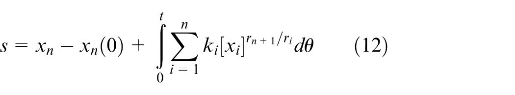
A novel terminal sliding mode surface for system (11) is designed as

$$s=x_n-x_n\left(0\right)+\underset{0}{\overset{t}{\int }}\sum _{i=1}^n{k}_i{\left[x_i\right]}^{r_{n+1}/r_i}d\theta$$

(12)

where $r_i$ , $i=1,\dots ,n+1$ , is defined in equation (3); $x_n(0)$ is the initial value of $x_n$ ; and $k_1,\dots ,k_n>0$ are selected such that the polynomial $s^n+k_n{s}^{n-1}+\cdots +k_{2}s+k_1$ is Hurwitz.

Theorem 2

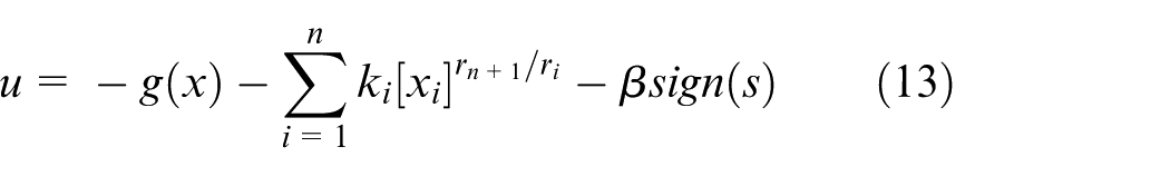
Consider the higher order nonlinear system (11) with the novel terminal sliding mode surface (12); if Assumption 3.1 holds, then system (11) can be globally stabilized in finite time under the following ITSMC law

$$u=-g\left(x\right)-\sum _{i=1}^n{k}_i{\left[x_i\right]}^{r_{n+1}/r_i}-\beta \mathrm{sign}\left(s\right)$$

(13)

where $\beta >0$ is a constant and satisfies $\beta >\mu$ .

Proof

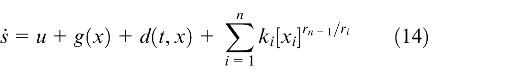
For the integral terminal sliding mode surface (12), the derivative of $s$ with respect to time $t$ along system (11) is

$$\stackrel{·}{s}=u+g\left(x\right)+d(t,x)+\sum _{i=1}^n{k}_i{\left[x_i\right]}^{r_{n+1}/r_i}$$

(14)

Substituting control law (13) into equation (14) yields

$$\stackrel{·}{s}=d(t,x)-\beta \mathrm{sign}\left(s\right)$$

(15)

Consider Lyapunov function $V=s^2/2$ . Taking the derivative of $V$ along system (11) under control law (13) gives

$$\stackrel{·}{V}=\mathrm{sd}(t,x)-\beta |s|\le -(\beta -\mu )|s|=-\lambda |s|$$

(16)

where $\lambda =\beta -\mu >0$ . Equation (16) implies that the ideal terminal sliding mode surface $s=0$ can be reached in finite time in spite of uncertainties and disturbances.

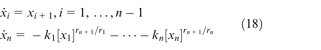
The ideal integral terminal sliding mode can be written as

$${\stackrel{·}{x}}_n=-k_1{\left[x_1\right]}^{r_{n+1}/r_1}-\cdots -k_n{\left[x_n\right]}^{r_{n+1}/r_n}$$

(17)

Combining equation (11) together with equation (17), we have

$$\begin{array}{c}\multicolumn{1}{c}{{\stackrel{·}{x}}_i=x_{i+1},i=1,\dots ,n-1}\\ \multicolumn{1}{c}{{\stackrel{·}{x}}_n=-k_1{\left[x_1\right]}^{r_{n+1}/r_1}-\cdots -k_n{\left[x_n\right]}^{r_{n+1}/r_n}}\end{array}$$

(18)

In Theorem 1, it is easy to show that equation (18) is globally finite-time stable. This completes the proof. □

In what follows, a numerical example is given to show the effectiveness of the proposed ITSMC method.

Example 2

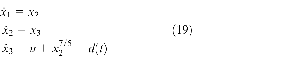
Consider the following system

$$\begin{array}{c}{\stackrel{·}{x}}_1=x_2\hfill \\ \begin{array}{c}{\stackrel{·}{x}}_2=x_3\hfill \\ \multicolumn{1}{c}{{\stackrel{·}{x}}_3=u+x_2^{7/5}+d\left(t\right)}\end{array}\hfill \end{array}$$

(19)

where $d(t)=0.5+0.5\sin (2t)$ .

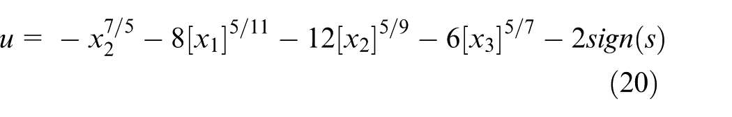
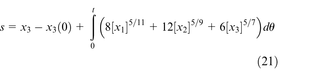
For system (19), we choose $\tau =-(2/11)$ , from which $r_1=1$ , then we have $r_2=9/11,r_3=7/11,r_4=5/11$ . We choose $k_1=8,k_2=12,k_3=6$ and $\beta =2$ , and initial condition $(x_1(0),x_2(0),x_3(0))=(3,1,-3)$ . Obviously, $|0.5+0.5\sin (2t)|<2$ , and Assumption 3.1 holds. According to Theorem 2, the control law can be designed as

$$u=-x_2^{7/5}-8{\left[x_1\right]}^{5/11}-12{\left[x_2\right]}^{5/9}-6{\left[x_3\right]}^{5/7}-2\mathrm{sign}\left(s\right)$$

(20)

where

$$s=x_3-x_3\left(0\right)+\underset{0}{\overset{t}{\int }}(8{\left[x_1\right]}^{5/11}+12{\left[x_2\right]}^{5/9}+6{\left[x_3\right]}^{5/7})d\theta$$

(21)

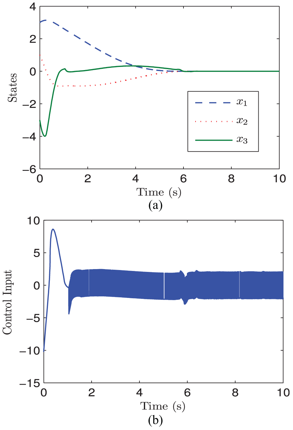
The responses of closed-loop systems (19) and (20) are shown in Figure 2. Figure 2(a) shows that control law (20) can stabilize system (19) rapidly. However, the discontinuity of control law (20) leads to undesired chattering in the control signal, which can be seen from Figure 2(b).

Figure 2.

The responses of the closed-loop systems (19) and (20). (a) The response curves of the states; (b) The response of the input signal.

Remark 3.1

It should be pointed out that if parameter $\beta$ in control law (13) is larger than the upper bound of disturbance $d(t,x)$ (i.e. $\beta >\mu$ ), the control law not only can suppress the external disturbances and parameter uncertainties but also can guarantee the states of the closed-loop system that reach the sliding mode in finite time. However, the signum function in control law (13) will bring undesired chattering. To reduce chattering, boundary layer method is usually adopted^3,8,56 in the literature. In Yu et al., ⁹ exponential reaching law is used to take place of constant speed reaching law, that is, $\mathrm{sign}(·)$ is replaced with $|·{|}^{\kappa }\mathrm{sign}(·),(0<\kappa <1)$ . However, both of the above two methods can only guarantee the finite-time reachability of the neighborhood of the sliding mode surface when there exist parameter uncertainties and disturbances. Therefore, finite-time stability cannot be guaranteed.

Chattering-free composite ITSMC law design

Finite-time disturbance observer (FTDOB) was first introduced in the study of Levant, ⁵⁷ which has a high efficiency in realizing nonlinear dynamical estimation and has been successfully used in missile guidance systems.^58,61 In order to estimate the total disturbance (here, the total disturbance includes parameter uncertainties and external disturbances) by using FTDOB, the following assumption is introduced.

Assumption 3.2

Given $d(t,x)\in {\mathbb{C}}^2$ , and there exists a constant $L>0$ such that $|\stackrel{··}{d}(t,x)|\le L$ .

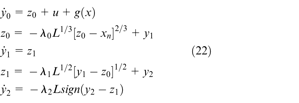
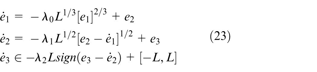
According to Levant ⁵⁷ and Assumption 3.2, we design the following FTDOB for system (11)

$$\begin{array}{c}\multicolumn{1}{c}{{\stackrel{·}{y}}_0=z_0+u+g\left(x\right)}\\ \multicolumn{1}{c}{z_0=-{\lambda }_0{L}^{1/3}{[z_0-x_n]}^{2/3}+y_1}\\ \multicolumn{1}{c}{{\stackrel{·}{y}}_1=z_1}\\ \multicolumn{1}{c}{z_1=-{\lambda }_1{L}^{1/2}{[y_1-z_0]}^{1/2}+y_2}\\ \multicolumn{1}{c}{{\stackrel{·}{y}}_2=-{\lambda }_2\mathrm{Lsign}(y_2-z_1)}\end{array}$$

(22)

By defining observer errors $e_1=y_0-x_n,e_2=y_1-d(t,x),e_3=y_2-\stackrel{·}{d}(t,x)$ , it follows from equations (11) and (22) that

$$\begin{array}{c}\multicolumn{1}{c}{{\stackrel{·}{e}}_1=-{\lambda }_0{L}^{1/3}{\left[e_1\right]}^{2/3}+e_2}\\ \multicolumn{1}{c}{{\stackrel{·}{e}}_2=-{\lambda }_1{L}^{1/2}{[e_2-{\stackrel{·}{e}}_1]}^{1/2}+e_3}\\ \multicolumn{1}{c}{{\stackrel{·}{e}}_3\in -{\lambda }_2\mathrm{Lsign}(e_3-{\stackrel{·}{e}}_2)+[-L,L]}\end{array}$$

(23)

where ${\lambda }_0$ , ${\lambda }_1$ , and ${\lambda }_2$ are appropriate positive constants.

Theorem 3

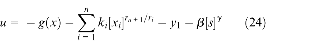
Consider the higher order nonlinear system (11) with the novel terminal sliding mode surface (12); if Assumption 3.2 holds, then system (11) can be globally stabilized in finite time under the following ITSMC law

$$u=-g\left(x\right)-\sum _{i=1}^n{k}_i{\left[x_i\right]}^{r_{n+1}/r_i}-y_1-\beta {\left[s\right]}^{\gamma }$$

(24)

where $\beta >0$ and $0<\gamma <1$ are parameters to be determined.

Proof

The proof of this theorem is divided into two steps: Inspired by Li and Tian, ⁵⁹ first we will show that under the proposed composite control law (24), the states of the closed-loop systems (11) and (24) are bounded in the time interval $[0,T_e]$ , where $T_e$ is the convergence time of the observer error system (23). While in the second step, we will show that the closed-loop systems (11) and (24) are globally finite-time stable.

• Step I: Taking the derivative of $s$ with respect to time $t$ along system (11) under control law (24) yields

$$\stackrel{·}{s}=-e_2-\beta {\left[s\right]}^{\gamma }$$

(25)

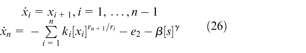
Substituting control law (24) into system (11) leads to

$$\begin{array}{c}{\stackrel{·}{x}}_i=x_{i+1},i=1,\dots ,n-1\hfill \\ \multicolumn{1}{c}{{\stackrel{·}{x}}_n=-\sum _{i=1}^n{k}_i{\left[x_i\right]}^{r_{n+1}/r_i}-e_2-\beta {\left[s\right]}^{\gamma }}\end{array}$$

(26)

Consider the following finite-time bounded (FTB) function for system (26)

$$U(s,x)=\frac{1}{2}(s^2+\sum _{i=1}^n{x}_i^2)$$

(27)

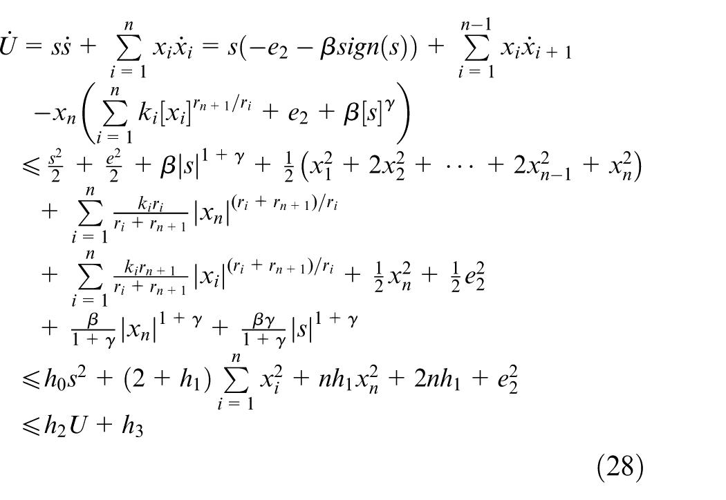
Note that $1\ge r_i>r_{i+1},i=1,\dots ,n,0<\gamma <1$ , then we have $1<((r_i+r_{n+1})/r_i)<2,i=1,\dots ,n,1<1+\gamma <2$ and $|x_i{|}^{r_i+r_{n+1}/r_i}<(1+x_i^2),|x_n{|}^{1+\gamma }<(1+x_n^2),|s{|}^{1+\gamma }<(1+s^2),\mathrm{for}\forall x_i\in R,s\in R$ . Taking the derivative of $U$ along the system (26) yields

$$\begin{array}{c}\stackrel{·}{U}=s\stackrel{·}{s}+\sum _{i=1}^n{x}_i{\stackrel{·}{x}}_i=s(-e_2-\beta \mathrm{sign}\left(s\right))+\sum _{i=1}^{n-1}{x}_i{\stackrel{·}{x}}_{i+1}\hfill \\ \multicolumn{1}{c}{-x_n(\sum _{i=1}^n{k}_i{\left[x_i\right]}^{r_{n+1}/r_i}+e_2+\beta {\left[s\right]}^{\gamma })}\\ \multicolumn{1}{c}{\le \frac{s^2}{2}+\frac{e^2}{2}+\beta |s{|}^{1+\gamma }+\frac{1}{2}(x_1^2+2x_2^2+\cdots +2x_{n-1}^2+x_n^2)}\\ \multicolumn{1}{c}{+\sum _{i=1}^n\frac{k_i{r}_i}{r_i+r_{n+1}}|x_n{|}^{(r_i+r_{n+1})/r_i}}\\ \multicolumn{1}{c}{+\sum _{i=1}^n\frac{k_i{r}_{n+1}}{r_i+r_{n+1}}|x_i{|}^{(r_i+r_{n+1})/r_i}+\frac{1}{2}{x}_n^2+\frac{1}{2}{e}_2^2}\\ \multicolumn{1}{c}{+\frac{\beta }{1+\gamma }|x_n{|}^{1+\gamma }+\frac{\beta \gamma }{1+\gamma }|s{|}^{1+\gamma }}\\ \multicolumn{1}{c}{\le h_0{s}^2+(2+h_1)\sum _{i=1}^n{x}_i^2+n{h}_1{x}_n^2+2n{h}_1+e_2^2}\\ \multicolumn{1}{c}{\le h_{2}U+h_3}\end{array}$$

(28)

where $h_0=(1/2)+(\beta /1+\gamma )+\beta$ , $h_1=\underset{i=1,\dots ,n}{\max }\{(r_i+r_{n+1})/r_i\}$ , $h_2=2\max \{h_0,2+(n+1)h_1\}$ , and $h_3=2n{h}_1+e_2^2$ (in equation (28), the famous Young’s inequality is used repetitively). According to Levant, ⁵⁷ system (23) will converge to the origin in finite time, which implies that $e_i,i=1,2,3$ are bounded, and then $h_3$ is bounded. It follows from equation (28) and Li and Tian ⁵⁹ that the FTB function $U(s,x)$ are bounded in the time interval $[0,T_e]$ ; thus, the states of the closed-loop systems (11) and (24) will not escape to infinity as $t\le T_e$ .

• Step II: As $t\ge T_e$ , $e_2=0$ , then equation (25) reduces to

$$\stackrel{·}{s}=-\beta {\left[s\right]}^{\gamma }$$

(29)

If follows from equation (29) and $V=(1/2)s^2$ that

$$\stackrel{·}{V}=-\beta s{\left[s\right]}^{\gamma }=-2^{(1+\gamma )/2}\beta V^{(1+\gamma )/2}$$

(30)

Therefore, under the proposed composite control law (24), the states of the closed-loop systems (11) and (24) will reach $s=0$ in finite time.

On $s=0$ , system (26) reduces to system (18). It is derived from Theorem 1 that equation (18) is finite-time stable. □

Example 3

We still take system (19) as an example to show the effectiveness of the control law (24).

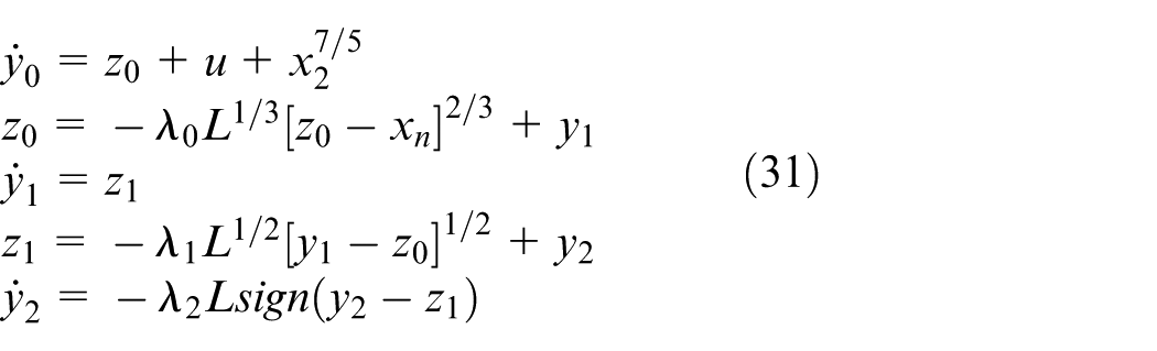
According to equation (22), the following FTDOB is designed for system (19)

$$\begin{array}{c}{\stackrel{·}{y}}_0=z_0+u+x_2^{7/5}\hfill \\ \multicolumn{1}{c}{z_0=-{\lambda }_0{L}^{1/3}{[z_0-x_n]}^{2/3}+y_1}\\ \multicolumn{1}{c}{{\stackrel{·}{y}}_1=z_1}\\ \multicolumn{1}{c}{z_1=-{\lambda }_1{L}^{1/2}{[y_1-z_0]}^{1/2}+y_2}\\ \multicolumn{1}{c}{{\stackrel{·}{y}}_2=-{\lambda }_2\mathrm{Lsign}(y_2-z_1)}\end{array}$$

(31)

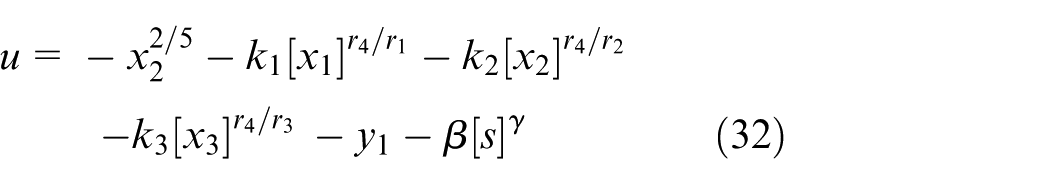
Furthermore, in Theorem 3, the following continuous ITSMC is constructed

$$u=-x_2^{2/5}-k_1{\left[x_1\right]}^{r_4/r_1}-k_2{\left[x_2\right]}^{r_4/r_2}-k_3{\left[x_3\right]}^{r_4/r_3}-y_1-\beta {\left[s\right]}^{\gamma }$$

(32)

for system (19).

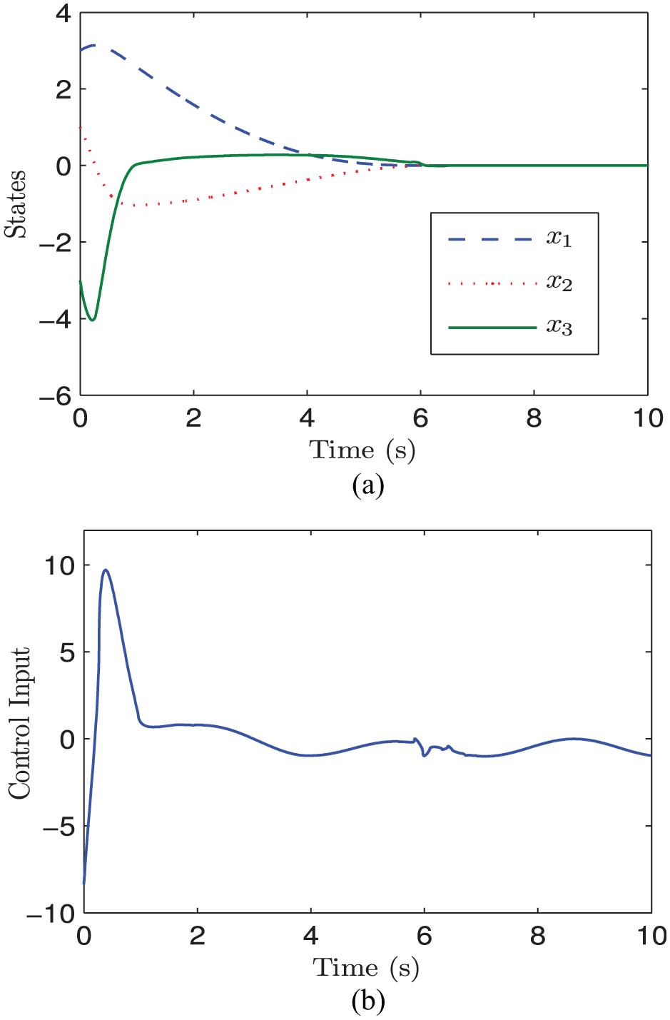
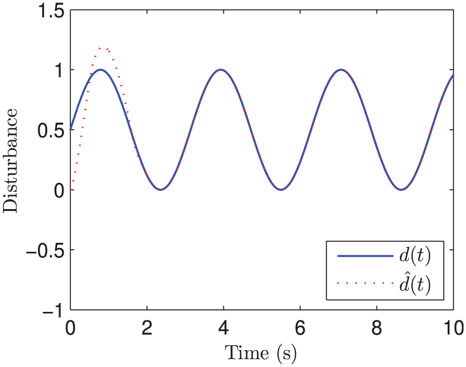
In simulation, we choose parameter values and initial conditions as $\tau =-(2/11),r_1=1,r_2=9/11,r_3=7/11,r_4=5/11,k_1=8,k_2=12,k_3=6,\beta =2,\gamma =3/5,{\lambda }_0=3,{\lambda }_1=1.5,{\lambda }_2=1.1$ and $(x_1(0),x_2(0),x_3(0))=(3,1,-3),(y_0(0),y_1(0),y_2(0))=(-3,0,0)$ . The simulation results are shown in Figures 3 and 4. It can be observed from Figure 3(a) that under the control law (32), the states of system (19) converge to the origin rapidly in spite of the disturbance. Figure 3(b) shows the responses of the input signal, which demonstrates that the proposed control law is chattering free. The responses of the real value and its estimated value of disturbance are shown in Figure 4, and it is observed that FTDOB can estimate the disturbance quickly and efficiently.

Figure 3.

The responses of the closed-loop systems (19) and (32). (a) The response curves of the states; (b) The response curve of the control signal.

Figure 4.

The real value ( $d(t)$ , the solid line) and the estimated value ( $\hat{d}(t)$ , the dotted line) of disturbance.

Conclusion

The ITSMC problem for a class of higher order nonlinear systems has been studied in this article. The main contribution of this article lies in the following aspects: (a) a novel FTC law with a simple structure has been proposed for a chain of integrators by using weighted homogeneity theory; (b) inspired by the proposed novel FTC law, a novel ITSMC law has been proposed for a class of higher order nonlinear systems; and (c) based on FTDOB technique and ITSMC approach, a chattering-free composite control law has been proposed for a class of higher order nonlinear systems in spite of parameter uncertainties and external disturbances.