Sage Journals: Discover world-class research

Abstract

In industrial and medical laboratories, prior to initiating the daily test procedure, the accuracy of the system is observed by measuring the reference control values. Measurements and test results may be below or above the reference value. Hence, the control data is employed in order to ensure that the test scores lie in the targeted range values, and the results obtained from the control data are evaluated via computer-based analysis. The results of the analysis have significant importance for control and improvement of process. Furthermore, the data to be analyzed may be the test results of a product as well as the measurement outcomes obtained from a laboratory. In this study, an algorithm named as Adaptive Precision Point Algorithm is proposed to evaluate the control data and to increase the stability by reducing the loss. In this schema, the contribution to the reduction of the total systematic error was observed by calculating the target working point and the Adaptive Precision Point deviations. Measurement outputs, in other terms the data, are processed in Adaptive Precision Point Algorithm. The algorithm determines a new adaptive working point for the incoming data by doing the required computations for precision working point. Moreover, the deviation between adaptive working point and the specified working point, which is defined according to the standards and rules, is calculated. By this way, adaptive working point is being utilized throughout the reduction of systemic errors. According to the results of the research, Adaptive Precision Point Algorithm eliminates the systematic errors on a large scale. The suggested algorithm provides results within the accepted quality deviation limits so it does not form a negativity in the understanding of quality. It is also observed that the algorithm sets a positive correlation between the minimized test results and reduction of time and material usage. Furthermore, the research and the algorithm offer a cost-effective solution. Consequently, the contribution and significance of the proposed algorithm can be understood in a better way by considering that it does not only maintain the quality limits but it also minimizes the cost and time spent during the testing of thousands of laboratory samples.

Keywords

Control data Adaptive Precision Point Algorithm internal quality control error correction

Introduction

Studies in the field of informatics play an important role throughout the stages of producing, storing, and processing the data in industrial and medical laboratories. The data which are subjected to the results of measurement and test give an idea of the quality of the laboratory. As is known, in order to verify the tests, certified reference control materials are being employed.^1,2 Furthermore, the control data are obtained by measuring these materials and the accuracy of the measurement is interpreted by comparing the control data with the reference values in the certificates. It is a well-known fact that the factors such as calibration, preventive maintenance, trainings, material–material qualities, and the environmental conditions that affect the control data result in errors. These faults which cause pecuniary and non-pecuniary losses affect the accuracy and quality of measurements. One of the primary aims and contributions of this study is to detect faulty control data that is out of limits on the results of measurement, on real time.^3,4 Hence, determining the type and source of errors by analyzing them is one of the important problems to be solved.^5–7 Meanwhile, the errors are addressed in two classes: (1) random and (2) systematic.^8,9 Random errors affect the process output instantaneously while the systemic ones do it continuously.^10,11 Another important useful outcome of our proposed model is that this work enables to conclude whether the faulty data is random or systematic by defining the type of errors detected.^12,13 Mistakes sourced from incorrect sampling, lack of attention, and instantaneous voltage change are examples of random errors. On the other hand, errors such as incorrect calibration, incorrectly conditioned test environment (i.e. high or low ambient temperature, out of limit humidity, and light), and human factor can be counted as the examples of systematic errors. The detection and correction of the effects caused by errors on the measurement results is an open and vital research topic.^14,15 In this study, by isolating the error types from the results, it is now possible for the working system to be able to control itself constantly and have a capability of self-correction. This is believed to be a significant contribution to the literature. This feature provides a cost-effective and efficient solution.

Figure 1 shows an example of systematic error. In Figure 1, the shift between the ideal operating point and the measured value is shown as Δwp (working point). The amount of shifting that occurs to the right or left of the ideal working point is shaped by the systematic error.

Figure 1.

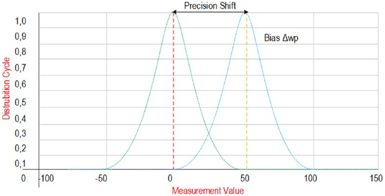
Systematic shift between the ideal working point and measured value—∆wp.

The concept of quality, which began to be used in Japan and America in 1950s, now has an indispensable importance in many sectors such as health, industry, service, and transportation.⁷ The quality process is governed by the software, test, and measurement technologies which organize standard-compliant production, measurement, and operating conditions. The quality of the laboratory is measured with the help of these technologies.^16,17 Furthermore, statistical quality control methods and standards are used in order to measure test quality in medical laboratories.⁷ It should be noted that the Clinical Laboratory Improvement Amendments (CLIA 88), College of American Pathologists (CAP), the International Quality Assurance Services (UK), the International Quality Assurance Services (UK), INSTAND (Germany), EUCAST (European Committee on Antimicrobial Susceptibility Testing), and similar institutions take place throughout the establishment and supervision of these methods and standards.¹⁸

Rule of quality control

The concept of quality control is an indication of the deviation of the measurement result from the expected values and errors that cause these deviations are evaluated by internal and external control mechanisms.^5,16 Internal quality control is an internal assessment that is not internationally validated by the laboratory using reference control material. Therefore, external quality control must be carried out by the accredited organizations in order for the laboratory’s control results to be valid in international manner.

Parameters affecting control data

The leading factors affecting the control data used for quality control cover various metrics such as accuracy, trueness, precision, interference, limit of detection (LoD), limit of quantitation (LoQ), linearity, uncertainty, reproducibility, duration of measurement, and robustness.^19,20 Moreover, the metrics of accuracy and precision have a critical importance in order to validate whether the results are in concordance with the expected reference values.

By definition, the accuracy is the measure of closeness between the reference value and the measured value, whereas the precision is defined as retrieving same results from repeated measurements.²¹ Likewise, the Gaussian curve depicted in Figure 2 is used to represent accuracy and precision. Note that the results under this curve constitute the accuracy while the normal at the center of the curve represents the precision.²² Besides, the methods such as OPSpec and Six Sigma are employed in order to measure the process performance of accuracy and precision analysis.^10,20,23

Figure 2.

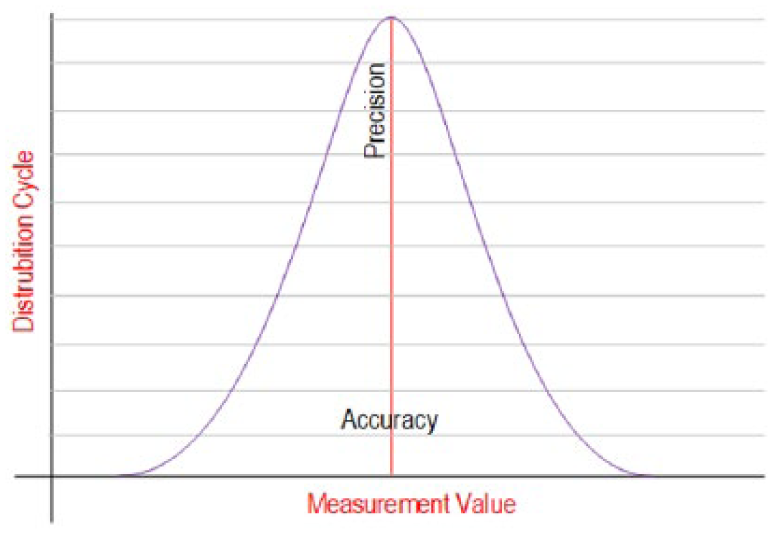
Accuracy and precision values in terms of measurement frequency and value.

Control chart and control limits

Visual control charts involving deviation values and upper and lower bounds are utilized for easy interpretation of the measurement data. Control charts are also widely used to determine the number of control data and control rules. The control data are evaluated according to time and working order by placing them on the chart and determining whether they are within the upper and lower limits.^11,24 Having the control data appear within the specified ranges indicates the conformity while the opposite case shows non-conformance.

Measuring the quality of models

For the measurement of the quality models, the models of P-A-F (Prevention-Appraisal-Failure), Crosby, Opportunity Cost, Process Cost, and ABC (Activity-Based Costing) are commonly employed.^21,23 Note that their efficiencies are measured by considering the parameters of prevention, appraisal, failure, and conformity. The above stated models and their efficiency classes are given in Table 1.

Table 1.

Models for quality data evaluation and their efficiency classes.

Model	Efficiency classes
P-A-F	{Prevention; Appraisal; Failure}
Crosby	{Prevention; Appraisal; Failure; Conformity}
Opportunity cost	{Valid, Invalid; Conformity; Abstract; Concrete}
Process cost	{Valid; Invalid}
ABC	{Significant; Insignificant}

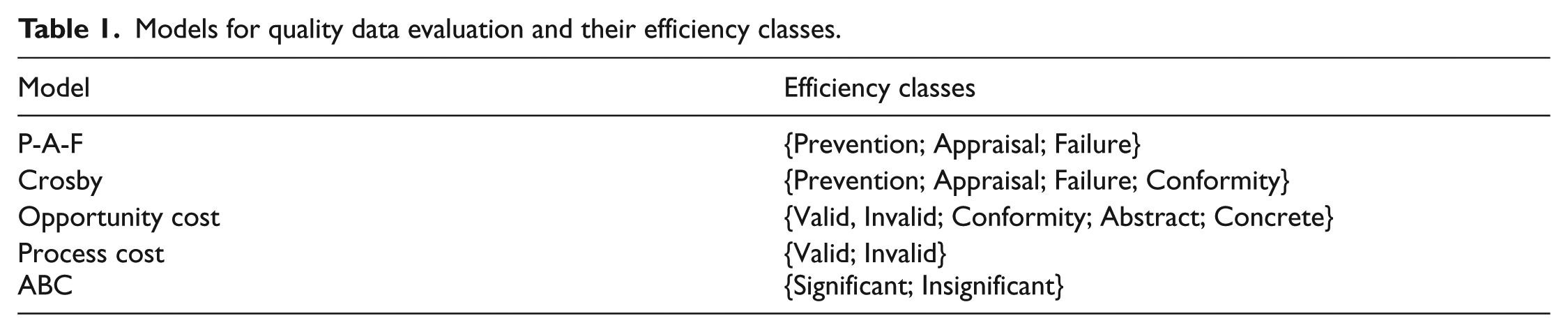
The P-A-F Model, accepted by the American Society for Quality Control and the British Standard Institute, is vulnerable to internal and external control failures and is partially inadequate in determining high costs, while reducing errors with prevention and appraisal processes.^25,26 On the other hand, according to the Crosby model, there exist conformity and error costs toward achieving quality. While the cost of adaptation represents the costs incurred for the requirements of the qualification, the cost of error represents the costs incurred when the targeted outcome cannot be achieved. Besides, the Opportunity Cost Model attaches importance to the transformation of opportunities and expectations in total quality process. For instance, the morale of an employee, the loss of work power, and gaining or losing the trust of the customer can be expressed by this model. Apart from the other models, the Process Cost model focuses on the total quality of the whole process. Compared to P-A-F model, the correction steps in the process can be identified in an easier fashion while it takes more time to observe repeated results obtained by connected processes. With the establishment of ABC model, activity-based measurement approach has been developed in which the quality is measured in terms of accuracy and precision.²⁷

Test life cycle

The test life cycle (TLC), which starts with test preparation and ends up with the valuation of the results, is shown in Figure 3.

Figure 3.

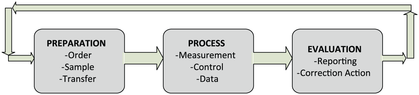
Test life cycle.

During the preliminary phase of TLC, preoperational preparations such as pre-measurement request and transfer are carried out and it is passed to process phase. Data for measurement, observation, and control are generated during the process phase in which digital data emerge. Nonetheless, achieving cost efficiency at this phase, which focuses on performance improvement, is a difficult problem.²⁸ For the performance centric purposes, analytical errors in the control data are analyzed.²⁹ The process is repeated until the errors are brought to a predetermined acceptable level and the estimated results are obtained in order to carry out the evaluation phase for the next stage. Next, the results obtained during the evaluation phase are reported and distributed.

In this study, a new approach which targets cost-effective improvement of the random and systematic errors that are dealt with in the TLC process phase is proposed. The proposed approach named as adaptive stable working point (ASWP) enables to use Westgard rules to identify the random errors in industry for the first time. With the proposed approach, moreover, it is aimed to create a cost-effective solution with a correct, effective, sustainable, and developable TLC.

Method

The proposed approach attempts to correct random and systematic error factors affecting the control data without deviating from the targeted quality values. In order to achieve this, datasets consisting of different numbers of control data have been employed. Application steps of the proposed model are given in Table 2.

Table 2.

Application phases of adaptive stable working point.

Level	Step	Processes carried out
D₀ (Data entry level)	1.1	Classify the data in dataset of X (Order, Time, Control data)
	1.2	Determine the data working group (Glucose, Cholesterol, Urea, etc.)
	1.3	Assign CLIA reference data value to workgroup
	1.4	Compute UCL (upper control limit) and LCL (lower control limit) for the L-J Chart
	1.5	Create L-J chart for WG rules
D₁ (Computation level)	2.1	Calculate the mean for the set of n elements, $\bar{x}$
	2.2	Compute the SD (standard deviation), CV-uncertainty, and deviation accuracy (bias)
	2.3	Calculate the absolute difference between the Cwp (computed working point) and Iwp (ideal working point), ∆wp
	2.4	Calculate the variance
	2.5	Specify AV (adaptation coefficient) by use of ∆wp and SD
	2.6	Specify ASWP (adaptive stable working point) for the X dataset and generate the chart
	2.7	Calculate the systematic error for X dataset
	2.8	Run WG rule filter for the $x_{k}$ singular values, detect the outlier data, and compute the random error
	2.9	Set the value of Recycle to 0 for the outlier data
	2.10	Discard the cases having Recycle = 0 for newly cases and go to step 2.1 for the new iteration
D₂ (Interpretation) level)	3.1	Notify the outlier-discard $x_{k}$ data, random and systematic error, coefficient of correction for the X dataset along with its gradient
D₂ (Interpretation) level)	3.2	Re-compute the algorithm for new cases. Show the AV coefficient for the kth iteration (ideal = 0), observe the convergence to 0. If AV ≤ ±0.1 then end the loop

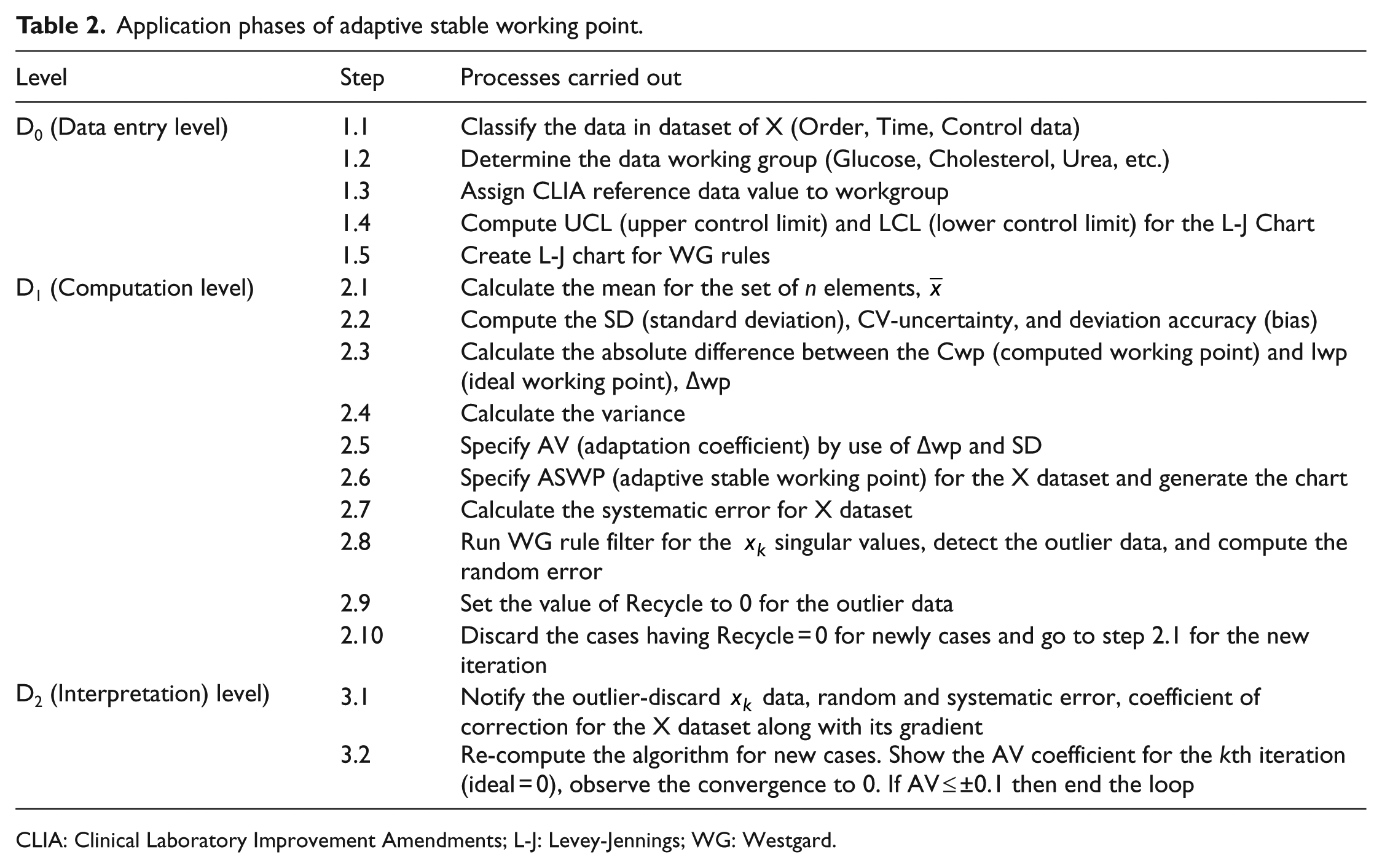
CLIA: Clinical Laboratory Improvement Amendments; L-J: Levey-Jennings; WG: Westgard.

Experimental studies

Implementation of the Westgard rules and generation of Levey-Jennings charts were achieved using a desktop computer with Intel Pentium dual core 2.6 GHz processor running Windows 10. Furthermore, the software MATLAB was employed to model and calculate the gain curves of the experimental data.

Levey-Jennings charts

Levey-Jennings, shortened as L-J, charts are generated for the dataset by considering all new $x_{k}$ data. Next, in the generated chart, the $\bar{x}$ (mean) and standard deviation (SD) curves obtained for the CLIA and the actual dataset are determined.³⁰ The distributions in the dataset are located in L-J chart and visual emphasis for each data is provided and analyzed far away from the mean. With the help of the Westgard rules, the analysis is conducted and used for random error detection.

Implementation of Westgard rules

We utilized the rules which were suggested by JO Westgard³¹ in order to evaluate the control results in statistical manner. Westgard rules were widely used in laboratory measurement and control systems to analyze the results (Figure 4).^31,32 First, we consider the error throughout the control process. As is known, OPSpecs chart, which is a method existing in the literature, constitutes a relation between the quality and accuracy of the conducted tests. Given the number of measurements, N, probability of error detection (Ped) and probability of false rejection (Pfr) are calculated.³³ Next, based on these calculations, we compute the SD, coefficient of variation (CV), and bias values.^23,34 The main parameters in which we use Westgard rules are the precomputed parameters such as SD, CV, and control limits.³² For the random error prediction, in particular, we have carried out our analysis via the rules proposed by Westgard and applied it into the dataset. 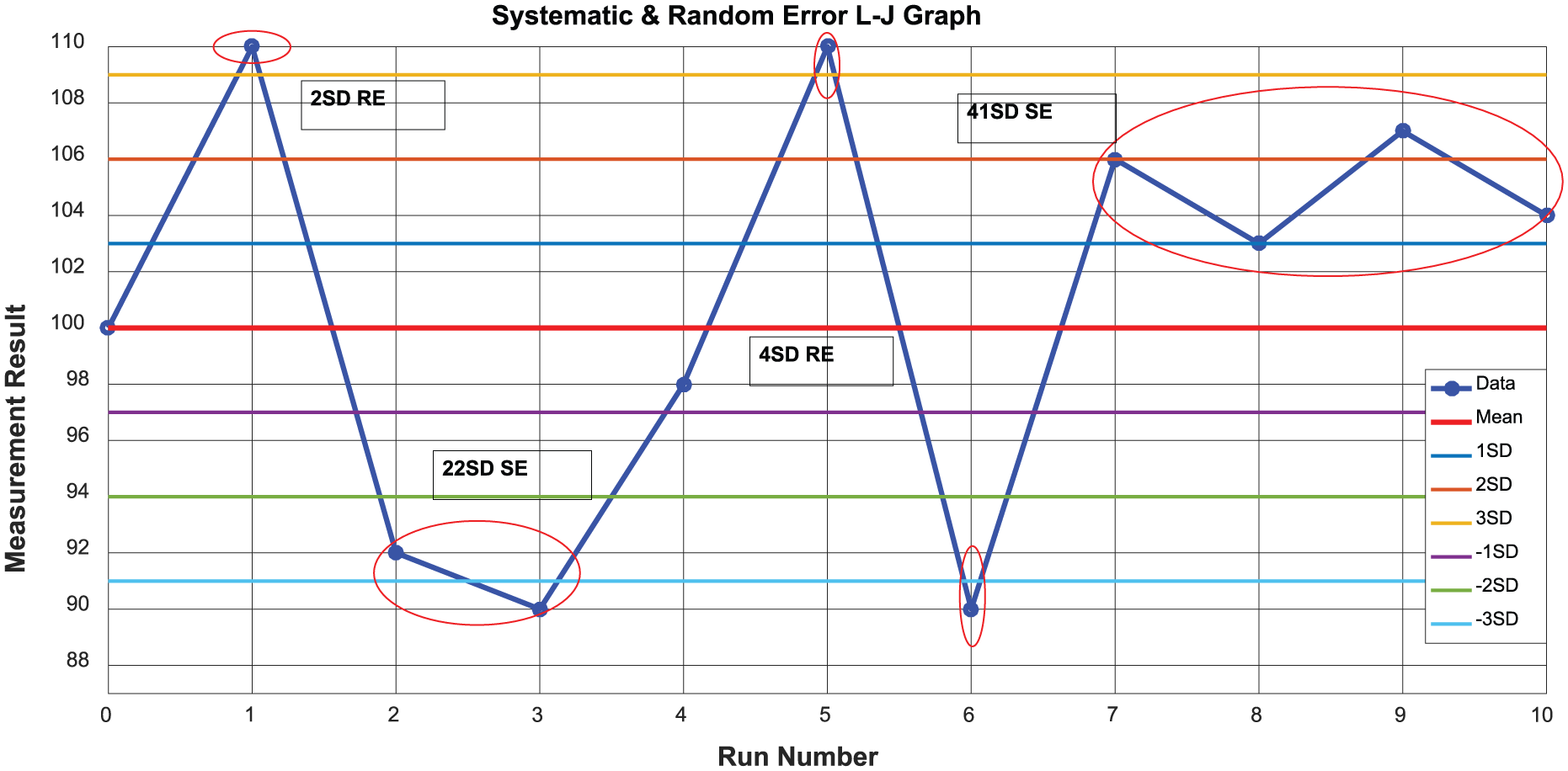Throughout the random error detection, if the singular data of $x_{k}$ in the dataset is flagged as “outlier-reject,” we set it to 0 in the re-evaluation process and discard for further computations.

Figure 4.

Application of the Westgard rules on the Levey-Jennings chart.

Generating the dataset

In this study, the actual laboratory control test results which have ethics committee approval were used as the base dataset. Besides, we have employed the standard reference values—which are used to verify the accuracy of the system prior to daily tests—as the control values. The control data is read from the device and recorded along with their timestamps. With this information, a table of control data for the laboratory and the test being studied is obtained. A sample dataset is presented in Table 3.

Table 3.

X Dataset example—actual test data.

Device: AU5800—Low Level 1—Glucose
Study date	Result	Min. value	Max. value	Unit	Average	Expected SD	Serum lot
18 April 2017, 09:19	101	86.75	119.25	mg/dL	103	8.125	0037F
17 April 2017, 09:11	99	86.75	119.25	mg/dL	103	8.125	0037F
14 April 2017, 09:11	100	86.75	119.25	mg/dL	103	8.125	0037F
13 April 2017, 09:01	101	86.75	119.25	mg/dL	103	8.125	0037F
12 April 2017, 09:01	102	86.75	119.25	mg/dL	103	8.125	0037F
11 April 2017, 08:44	102	86.75	119.25	mg/dL	103	8.125	0037F
10 April 2017, 09:40	101	86.75	119.25	mg/dL	103	8.125	0037F
07 April 2017, 09:14	99	86.75	119.25	mg/dL	103	8.125	0037F
06 April 2017, 09:07	102	86.75	119.25	mg/dL	103	8.125	0037F
05 April 2017, 09:28	100	86.75	119.25	mg/dL	103	8.125	0037F
04 April 2017, 08:45	101	86.75	119.25	mg/dL	103	8.125	0037F
03 April 2017, 09:06	101	86.75	119.25	mg/dL	103	8.125	0037F
31 March 2017, 09:19	101	86.75	119.25	mg/dL	103	8.125	0037F
30 March 2017, 08:55	100	86.75	119.25	mg/dL	103	8.125	0037F
29 March 2017, 08:52	99	86.75	119.25	mg/dL	103	8.125	0037F
28 March 2017, 09:47	100	86.75	119.25	mg/dL	103	8.125	0037F
28 March 2017, 09:16	105	86.75	119.25	mg/dL	103	8.125	0037F
27 March 2017, 09:35	98	86.75	119.25	mg/dL	103	8.125	0037F
24 March 2017, 09:28	101	86.75	119.25	mg/dL	103	8.125	0037F
23 March 2017, 09:11	97	86.75	119.25	mg/dL	103	8.125	0037F
22 March 2017, 09:34	97	86.75	119.25	mg/dL	103	8.125	0037F
21 March 2017, 09:37	99	86.75	119.25	mg/dL	103	8.125	0037F
21 March 2017, 09:09	96	86.75	119.25	mg/dL	103	8.125	0037F
20 March 2017, 10:57	97	86.75	119.25	mg/dL	103	8.125	0037F
17 March 2017, 09:27	100	86.75	119.25	mg/dL	103	8.125	0037F
16 March 2017, 09:08	102	86.75	119.25	mg/dL	103	8.125	0037F
15 March 2017, 08:45	101	86.75	119.25	mg/dL	103	8.125	0037F
14 March 2017, 08:48	102	86.75	119.25	mg/dL	103	8.125	0037F
13 March 2017, 10:13	102	86.75	119.25	mg/dL	103	8.125	0037F
10 March 2017, 09:10	99	86.75	119.25	mg/dL	103	8.125	0037F

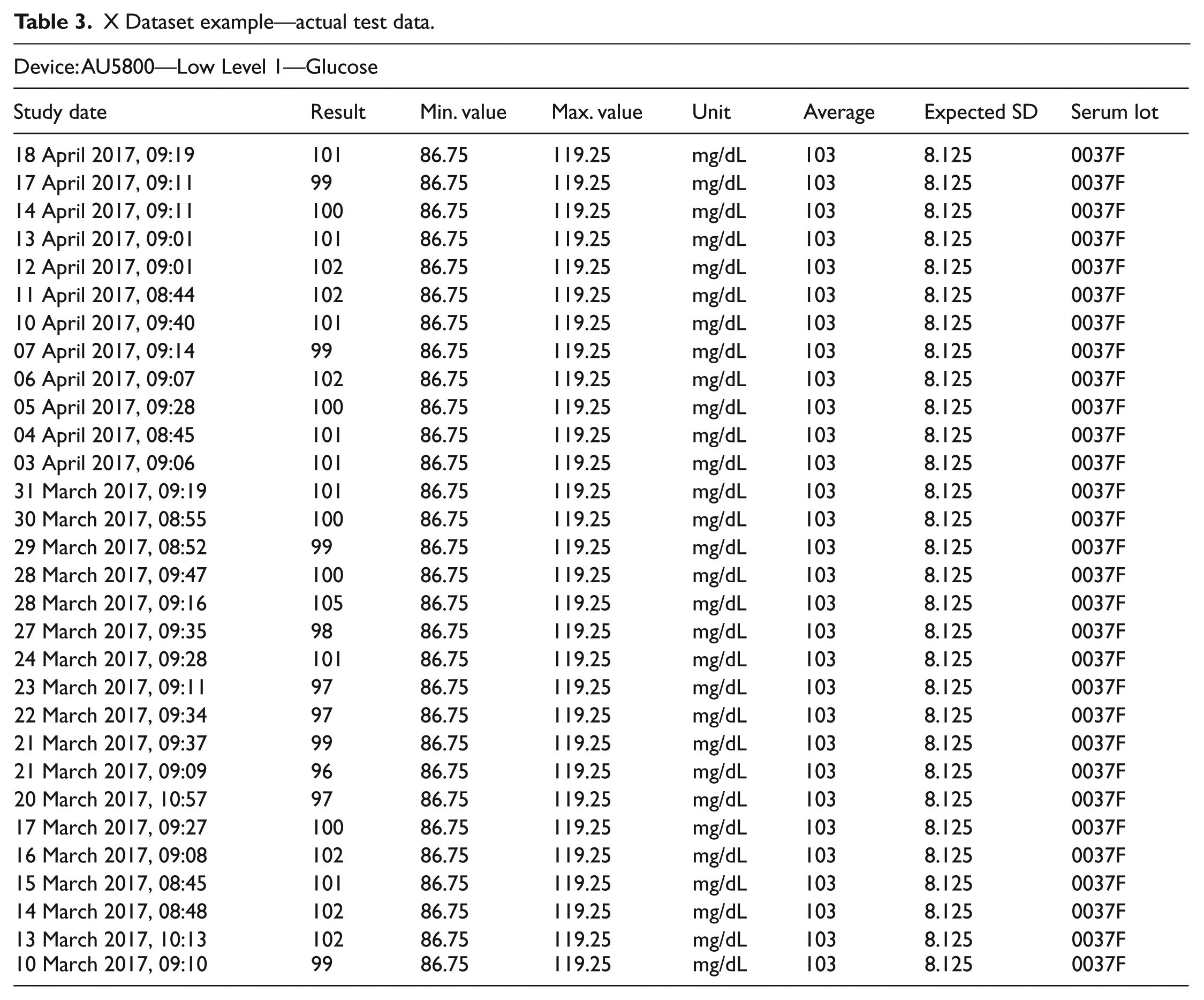
An excel chart was created for the glucose tests containing control data of 30 days obtained from the device. Moreover, the data from the table was used in the model flow process. As it can be seen from Table 3, minimum and maximum limit values refer to the lower and upper bounds of the standard control values. Thus, measurement results to be made in the system are expected to lie between these two limits. In this configuration, it should be noted that the average values constitute the control values themselves and there may be deviations from these values where the permitted SDs were indicated in Table 3. As presented in Table 3, the employed test device is AU5800 and it was used for low-level glucose test along with serum lot “0037F.”

Pre-analysis calculations

According to the range of distribution, variance-variability, SD, and CV are the required parameters to be computed prior to statistical interpretation and evaluation of the Gaussian curves drawn according to accuracy and precision values.^32,34,35 The calculation of SD is given in formula (1) below

S D = \sqrt{(\sum_{k = 1}^{n} {(x_{k} - \bar{x})}^{2}) / (k - 1)}

(1)

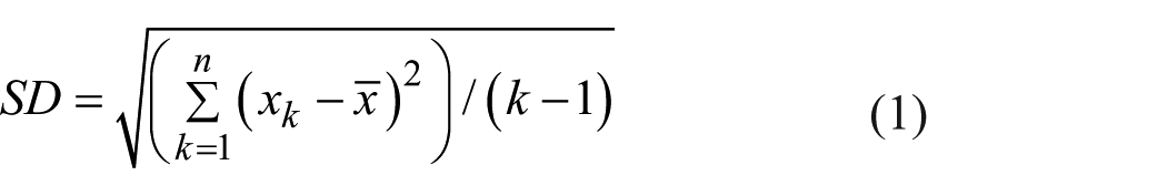
According to equation (1), n represents the total number of data in dataset, whereas $x_{k}$ indicates the kth data. Besides, $\bar{x}$ presents the value which can be computed by formula (2) below

\bar{x} = \sum_{k = 1}^{n} \frac{x_{k}}{k}

(2)

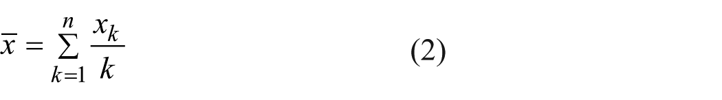
Moreover, the upper and lower control limits are calculated via formula (3) using the computed SD and mean values

(U c l, L c l) = \bar{x} \pm m S

(3)

The coefficient of m expresses the distribution of positive and negative sides of the SD and, in practice, it is often set to 1, 2, or 3.^36,37 Meanwhile, Levey-Jennings tables are constructed with the calculated values and the whole scattering is observed by plotting the control data on the table.^38,39 At this stage, we run the Westgard rules by taking into account the positioning of the data which are above and below the average values around the $\pm m S$ band.^40–43

Next, the value of ∆wp is computed by taking the difference of Cwp (calculated working point) and Iwp (ideal working point) using formula (4)

Δ wp = \bar{x} (Iwp) - \bar{x} (Cwp)

(4)

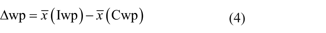
The direction of bias to the ideal, that is, bias direction, for the test results is determined according to whether Δwp is negative or positive. In this regard, if the result is positive, the working point shift takes place on the right side of the ideal, whereas it is on the left side for the opposite case. In Figure 5, right and left shifts are depicted on precision chart. This finding sheds light on the direction of the systematic error for the process using the equation below

Adaptation Value = Current Value - Previous Value

(5)

Figure 5.

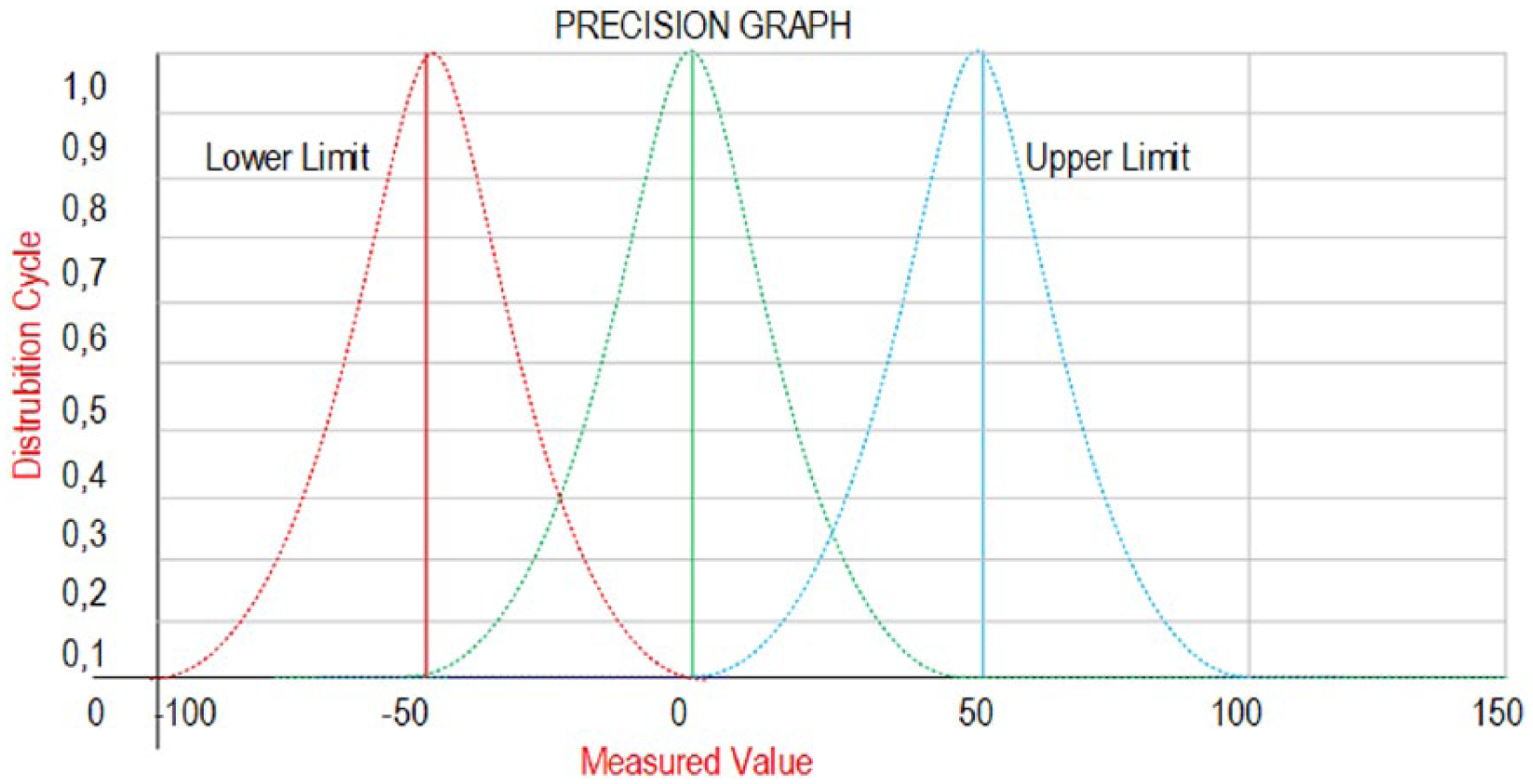
Shifting for the weighted averages of the calculated dataset according to the reference value.

As a result of applying the calculated adaptation value to the system, the correction for error reduction and the increase in the result accuracy are shown in the Accuracy–Error curve depicted in Figure 6. Thus, the measured error based on the initial control data obtained from the system and the resulting improvement by use of our model implementation are plotted as adaptation resultant error point. In Figure 6, the decrease in the error margin and the increase in accuracy are shown by applying the model. At this point, our expectation is generating the results using the control data closer to the point where the accuracy reaches to the value of 1. In contrast, it is also aimed that the results having too many errors should appear near to the point where the error reaches to the value of 1.

Figure 6.

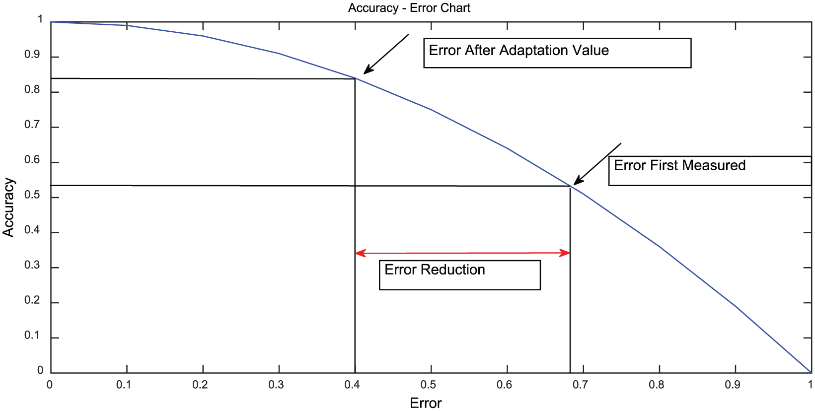
Error reduction effect of the proposed algorithm on accuracy-error chart.

Experimental works and results

Throughout the experiments, control data from the laboratory were processed with the reference Glucose values according to CLIA 88. For the glucose test, we have used the control value of ±6 mg/dL or the mean value of ±10% that were specified by the standards. Measurements were made with two devices—called as Device A and B—using the dataset shown in Table 3. It should be noted that these devices are in the same condition. The standard test kit certificate values used in the laboratory are given in Table 4 for device A. The results obtained according to these values are shown in Table 5.

Table 4.

Standard (reference) test kit values for Device A Glucose Level 1 Test.

AU5800 Device A—Low Level
Study date	Min. value	Max. value	Unit	Mean	SD	Serum lot
10 March to 18 April 2017	86.75	119.25	mg/dL	103	8.125	0037F

Table 5.

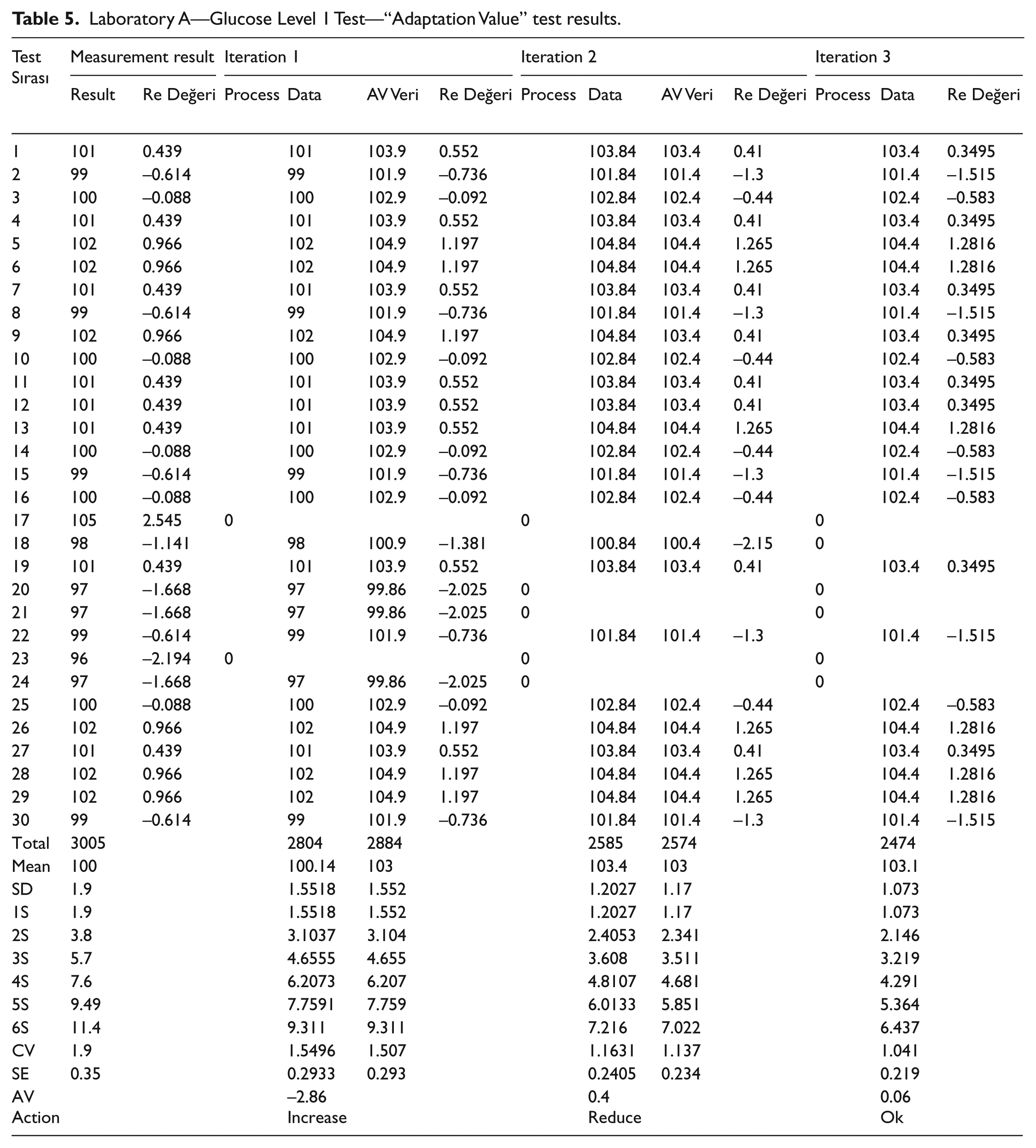
Laboratory A—Glucose Level 1 Test—“Adaptation Value” test results.

Test Sırası	Measurement result		Iteration 1				Iteration 2				Iteration 3
Test Sırası	Result	Re Değeri	Process	Data	AV Veri	Re Değeri	Process	Data	AV Veri	Re Değeri	Process	Data	Re Değeri
1	101	0.439		101	103.9	0.552		103.84	103.4	0.41		103.4	0.3495
2	99	−0.614		99	101.9	−0.736		101.84	101.4	−1.3		101.4	−1.515
3	100	−0.088		100	102.9	−0.092		102.84	102.4	−0.44		102.4	−0.583
4	101	0.439		101	103.9	0.552		103.84	103.4	0.41		103.4	0.3495
5	102	0.966		102	104.9	1.197		104.84	104.4	1.265		104.4	1.2816
6	102	0.966		102	104.9	1.197		104.84	104.4	1.265		104.4	1.2816
7	101	0.439		101	103.9	0.552		103.84	103.4	0.41		103.4	0.3495
8	99	−0.614		99	101.9	−0.736		101.84	101.4	−1.3		101.4	−1.515
9	102	0.966		102	104.9	1.197		104.84	103.4	0.41		103.4	0.3495
10	100	−0.088		100	102.9	−0.092		102.84	102.4	−0.44		102.4	−0.583
11	101	0.439		101	103.9	0.552		103.84	103.4	0.41		103.4	0.3495
12	101	0.439		101	103.9	0.552		103.84	103.4	0.41		103.4	0.3495
13	101	0.439		101	103.9	0.552		104.84	104.4	1.265		104.4	1.2816
14	100	−0.088		100	102.9	−0.092		102.84	102.4	−0.44		102.4	−0.583
15	99	−0.614		99	101.9	−0.736		101.84	101.4	−1.3		101.4	−1.515
16	100	−0.088		100	102.9	−0.092		102.84	102.4	−0.44		102.4	−0.583
17	105	2.545	0				0				0
18	98	−1.141		98	100.9	−1.381		100.84	100.4	−2.15	0
19	101	0.439		101	103.9	0.552		103.84	103.4	0.41		103.4	0.3495
20	97	−1.668		97	99.86	−2.025	0				0
21	97	−1.668		97	99.86	−2.025	0				0
22	99	−0.614		99	101.9	−0.736		101.84	101.4	−1.3		101.4	−1.515
23	96	−2.194	0				0				0
24	97	−1.668		97	99.86	−2.025	0				0
25	100	−0.088		100	102.9	−0.092		102.84	102.4	−0.44		102.4	−0.583
26	102	0.966		102	104.9	1.197		104.84	104.4	1.265		104.4	1.2816
27	101	0.439		101	103.9	0.552		103.84	103.4	0.41		103.4	0.3495
28	102	0.966		102	104.9	1.197		104.84	104.4	1.265		104.4	1.2816
29	102	0.966		102	104.9	1.197		104.84	104.4	1.265		104.4	1.2816
30	99	−0.614		99	101.9	−0.736		101.84	101.4	−1.3		101.4	−1.515
Total	3005			2804	2884			2585	2574			2474
Mean	100			100.14	103			103.4	103			103.1
SD	1.9			1.5518	1.552			1.2027	1.17			1.073
1S	1.9			1.5518	1.552			1.2027	1.17			1.073
2S	3.8			3.1037	3.104			2.4053	2.341			2.146
3S	5.7			4.6555	4.655			3.608	3.511			3.219
4S	7.6			6.2073	6.207			4.8107	4.681			4.291
5S	9.49			7.7591	7.759			6.0133	5.851			5.364
6S	11.4			9.311	9.311			7.216	7.022			6.437
CV	1.9			1.5496	1.507			1.1631	1.137			1.041
SE	0.35			0.2933	0.293			0.2405	0.234			0.219
AV				–2.86				0.4				0.06
Action				Increase				Reduce				Ok

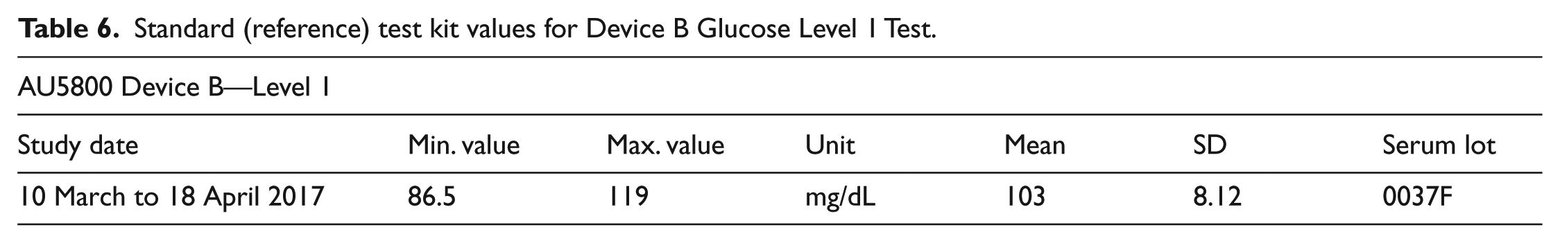
The standard values for the device B used for the measurement are given in Table 6, and the results obtained according to this are shown in Table 7.

Table 6.

Standard (reference) test kit values for Device B Glucose Level 1 Test.

AU5800 Device B—Level 1
Study date	Min. value	Max. value	Unit	Mean	SD	Serum lot
10 March to 18 April 2017	86.5	119	mg/dL	103	8.12	0037F

Table 7.

Laboratory A Glucose Level 1 Test—“Adaptation Value” test results.

Test Sırası	Measurement results		Iteration 1				Iteration 2				Iteration 3				Iteration 4
Test Sırası	Result	Re Değeri	Process	Data	AV Data	Re Değeri	Process	Data	AV Veri	Re Değeri	Process	Data	AV Veri	Re Değeri	Process	Data	AV Veri	Re Değeri
1	99	−0.91		99	101.2	−1.6		101.2	101.1	−1.9		101.1	101.3	−2.06	0
2	102	0.869		102	104.2	1.04		104.2	104.1	1.04		104.1	104.3	1.459		104.3	104.2	1.486
3	101	0.276		101	103.2	0.17		103.2	103.1	0.06		103.1	103.3	0.287		103.3	103.2	0.211
4	100	−0.32		100	102.2	−0.7		102.2	102.1	−0.9		102.1	102.3	−0.88		102.3	102.2	−1.06
5	104	2.054	0								0				0
6	102	0.869		102	104.2	1.04		104.2	104.1	1.04		104.1	104.3	1.459		104.3	104.2	1.486
7	101	0.276		101	103.2	0.17		103.2	103.1	0.06		103.1	103.3	0.287		103.3	103.2	0.211
8	101	0.276		101	103.2	0.17		103.2	103.1	0.06		103.1	103.3	0.287		103.3	103.2	0.211
9	103	1.461		103	105.2	1.92		105.2	105.1	2.02	0				0
10	100	−0.32		100	102.2	−0.7		102.2	102.1	−0.9		102.1	102.3	−0.88		102.3	102.2	−1.06
11	101	0.276		101	103.2	0.17		103.2	103.1	0.06		103.1	103.3	0.287		103.3	103.2	0.211
12	102	0.869		102	104.2	1.04		104.2	104.1	1.04		104.1	104.3	1.459		104.3	104.2	1.486
13	100	−0.32		100	102.2	−0.7		102.2	102.1	−0.9		102.1	102.3	−0.88		102.3	102.2	−1.06
14	101	0.276		101	103.2	0.17		103.2	103.1	0.06		103.1	103.3	0.287		103.3	103.2	0.211
15	103	1.461		103	105.2	1.92		105.2	105.1	2.02	0				0
16	102	0.869		102	104.2	1.04		104.2	104.1	1.04		104.1	104.3	1.459		104.3	104.2	1.486
17	100	−0.32		100	102.2	−0.7		102.2	102.1	−0.9		102.1	102.3	−0.88		102.3	102.2	−1.06
18	102	0.869		102	104.2	1.04		104.2	104.1	1.04		104.1	104.3	1.459		104.3	104.2	1.486
19	101	0.276		101	103.2	0.17		103.2	103.4	0.42		103.4	103.6	0.709		103.6	103.5	0.67
20	100	−0.32		100	102.2	−0.7		102.2	102.1	−0.9		102.1	102.3	−0.88		102.3	102.2	−1.06
21	97	−2.09	0				0				0				0
22	97	−2.09	0				0				0				0
23	97	−2.09	0				0				0				0
24	100	−0.32		100	102.2	−0.7		102.2	102.1	−0.9		102.1	102.3	−0.88		102.3	102.2	−1.06
25	101	0.276		101	103.2	0.17		103.2	103.1	0.06		103.1	103.3	0.287		103.3	103.2	0.211
26	100	−0.32		100	102.2	−0.7		102.2	102.1	−0.9		102.1	102.3	−0.88		102.3	102.2	−1.06
27	98	−1.5		98	100.2	−2.5	0				0				0
28	100	−0.32		100	102.2	−0.7		102.2	102.1	−0.9		102.1	102.3	−0.88		102.3	102.2	−1.06
29	101	0.276		101	103.2	0.17		103.2	103.1	0.06		103.1	103.3	0.287		103.3	103.2	0.211
30	100	−0.32		100	102.2	−0.7		102.2	102.1	−0.9		102.1	102.3	−0.88		102.3	102.2	−1.06
Total	3016			2621	2678			2578	2575			2365	2369			2268	2266
Mean	101			101	103			103.1	103			102.8	103			103.1	103
SD	1.7			1.14	1.144			1.017	1.02			0.853	0.853			0.784	0.784
1S	1.7			1.14	1.144			1.017	1.02			0.853	0.853			0.784	0.784
2S	3.4			2.29	2.288			2.033	2.04			1.707	1.707			1.568	1.568
3S	5.1			3.43	3.433			3.05	3.061			2.56	2.56			2.352	2.352
4S	6.8			4.58	4.577			4.067	4.081			3.413	3.413			3.137	3.137
5S	8.4			5.72	5.721			5.083	5.101			4.266	4.266			3.921	3.921
6S	10			6.87	6.865			6.1	6.121			5.12	5.12			4.705	4.705
CV	1.7			1.14	1.111			0.986	0.99			0.83	0.828			0.761	0.761
SE	0.3			0.22	0.224			0.203	0.204			0.178	0.178			0.164	0.164
AV				–2.2				0.11				–0.17				0.08
Act				Increase				Reduce				Increase				Reduce		OK

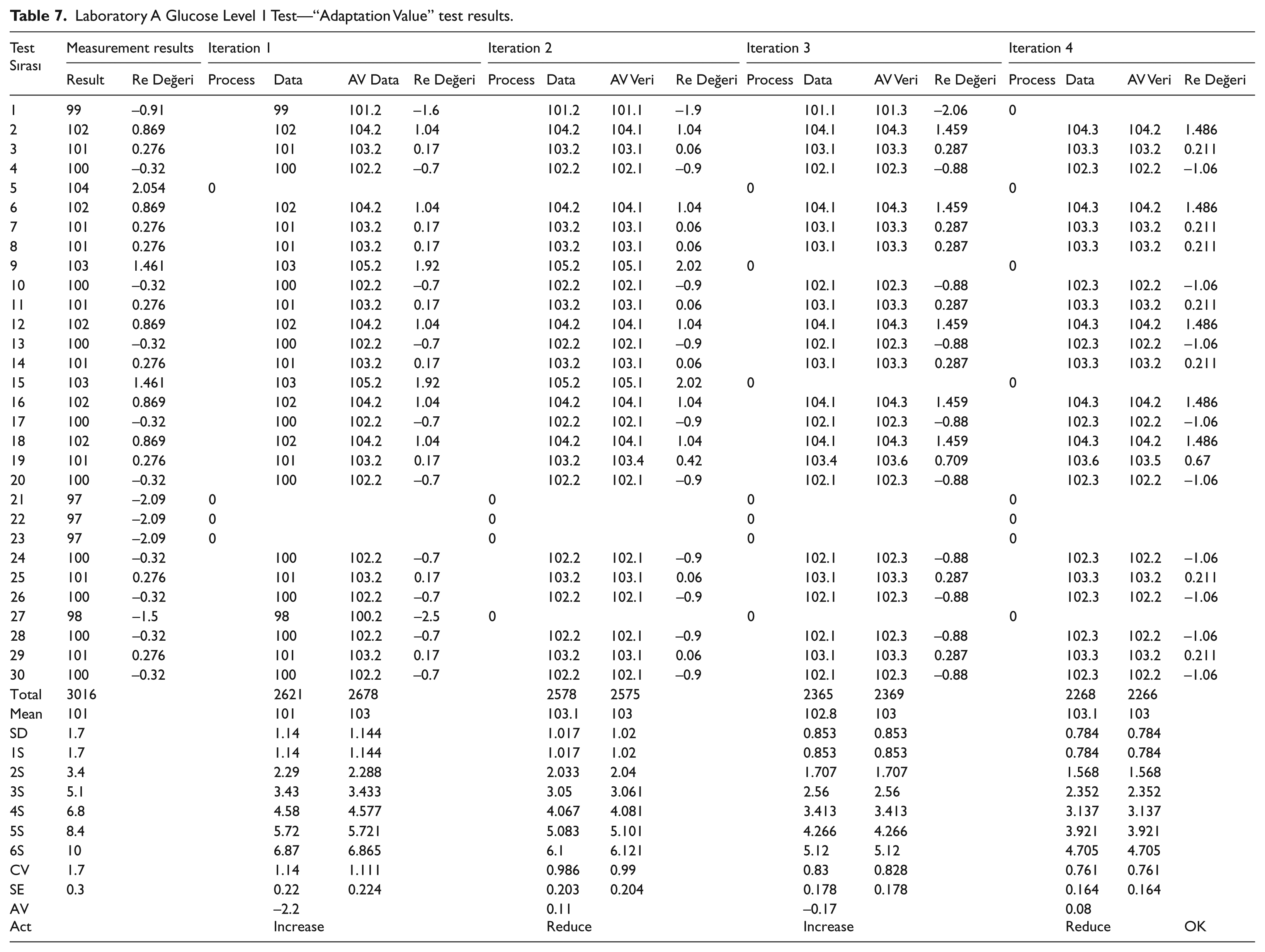
The model was applied to the data which have been collected in 30 days and it was listed in Table 7. For the first raw data, ±6 SD parameters are separately calculated to observe SD within SD, CV, standard error (SE), ±3 SD, and Six Sigma. For the first data, ±2 SD value (z-score) is calculated for each individual data. Note that, since the data above this value means a random error in the system, it has a destructive effect on the whole system. In the first step, random errors are detected and the systematic error contribution that the data group has in the next step is investigated. Next, the corresponding adaptation value (AV) is used to determine the magnitude and orientation of the adaptation quantity in order to reduce the systematic error. According to Table 7, having the negative sign of AV for the iteration result indicates that the dataset has shifted to the left from the ideal value, that is, the negative direction, and needs to shift to the right by the specified amount. On the other hand, the value of AV = +0.11 indicates that the dataset has shifted to the right-positive region with a systematic error and that this amount has to be shifted to the left.

For the experiment listed in Table 5, the results settled down to the ±2 SD band within three iterations. As a result, while 28 individual data were in ±1.9 SD distribution range at initial stage, it was found that 24 individual data were placed in the range of ±1.07 SD at the third iteration. Moreover, the initial CV value which was 1.9 reduced to 1.041 at the third iteration. We have also observed that the initial SE which was 0.35 has decreased to 0.22 at the end of the computation. Note that, for three iterations of this experiment, the adaptation values were suggested as 2.86 (increase), 0.4 (decrease), and 0.06 (decrease), respectively. In the last iteration, the process was terminated since the computed values fell within the expected deviation limits.

For the experiment listed in Table 7, the results settled down to the ±2 SD band within four iterations. While 26 individual data were in ±1.7 SD distribution range at initial stage, it was found that 22 individual data were placed in the range of ±0.78 SD at the fourth iteration. Besides, the initial CV value which was 1.7 reduced to 0.76 at the fourth iteration. Furthermore, initial SE which was 0.3 has decreased to 0.16 at the end of the process. For four iterations of this experiment, the adaptation values were determined as 2.2 (increase), 0.11 (decrease), 0.17 (increase), and 0.08 (decrease), respectively. Similar to the experiment given in the paragraph above, the process was terminated since the values in last iteration fell within the expected deviation limits.

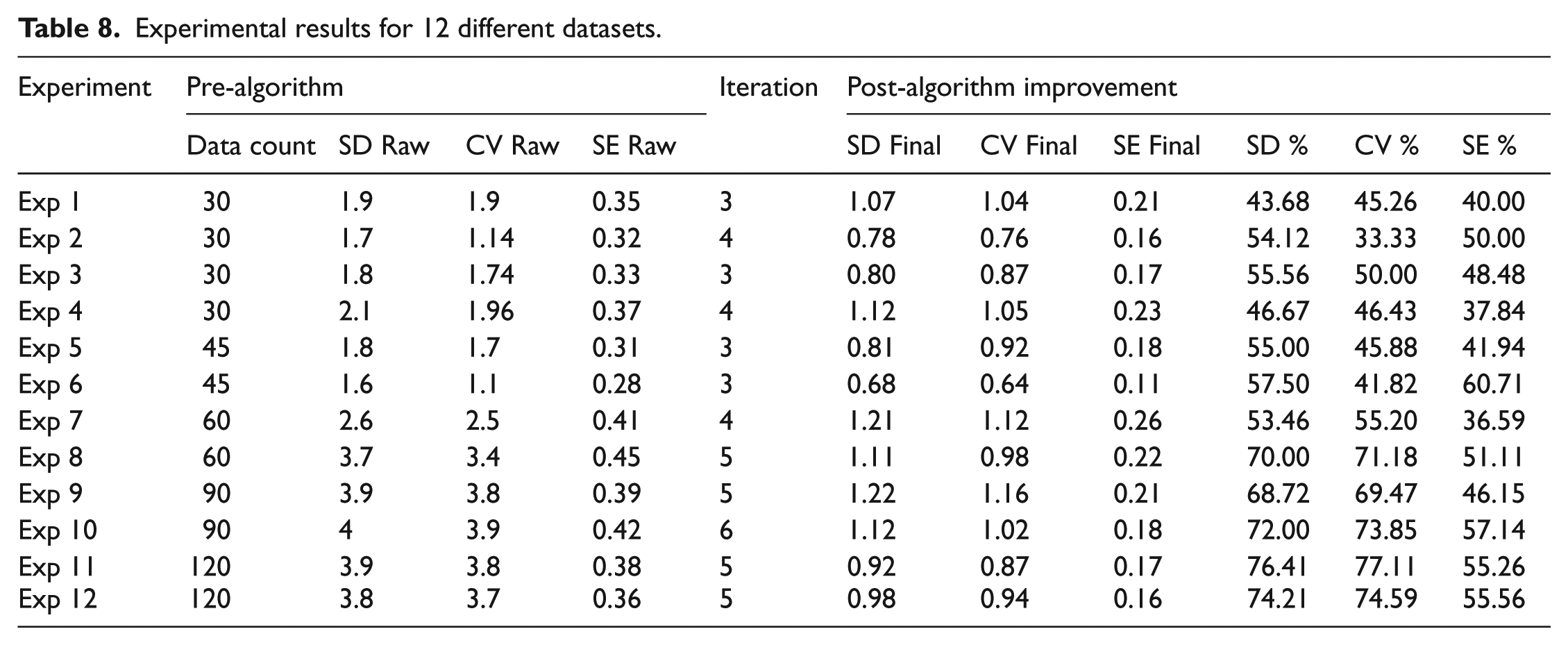
The results listed in Table 8 were obtained for a total of 12 different control data groups. For the control data of 12 different experiments, SD, CV, and SE values belonging to the raw data were calculated and listed. Moreover, random and systematic errors were detected. In each iteration, SD, CV, and SE values are recalculated and interpreted. Besides, iterations were terminated at the point where the adaptation value is 0.1 and below. At this step, the last SD, CV, and SE values obtained were listed. The error correction percentages obtained using Adaptive Precision Point Algorithm on initial data are given in the SE% column. For the group having 30 individual control data, correction ranging between 37.84% and 50.00% was obtained for the systematic error. Similarly, for the group having 45 individual control data, systematic error has been computed ranging from 41.94% to 60.71%, while it has been measured between 36.59% and 51.11% for the group having 60 data. These value ranges have been detected as 46.15% to 57.14% and 46.15% to 57.14% for the control datasets having 90 and 120 individual data, respectively.

Table 8.

Experimental results for 12 different datasets.

Experiment	Pre-algorithm				Iteration	Post-algorithm improvement
	Data count	SD Raw	CV Raw	SE Raw		SD Final	CV Final	SE Final	SD %	CV %	SE %
Exp 1	30	1.9	1.9	0.35	3	1.07	1.04	0.21	43.68	45.26	40.00
Exp 2	30	1.7	1.14	0.32	4	0.78	0.76	0.16	54.12	33.33	50.00
Exp 3	30	1.8	1.74	0.33	3	0.80	0.87	0.17	55.56	50.00	48.48
Exp 4	30	2.1	1.96	0.37	4	1.12	1.05	0.23	46.67	46.43	37.84
Exp 5	45	1.8	1.7	0.31	3	0.81	0.92	0.18	55.00	45.88	41.94
Exp 6	45	1.6	1.1	0.28	3	0.68	0.64	0.11	57.50	41.82	60.71
Exp 7	60	2.6	2.5	0.41	4	1.21	1.12	0.26	53.46	55.20	36.59
Exp 8	60	3.7	3.4	0.45	5	1.11	0.98	0.22	70.00	71.18	51.11
Exp 9	90	3.9	3.8	0.39	5	1.22	1.16	0.21	68.72	69.47	46.15
Exp 10	90	4	3.9	0.42	6	1.12	1.02	0.18	72.00	73.85	57.14
Exp 11	120	3.9	3.8	0.38	5	0.92	0.87	0.17	76.41	77.11	55.26
Exp 12	120	3.8	3.7	0.36	5	0.98	0.94	0.16	74.21	74.59	55.56

Conclusion

In this study, an algorithmic approach called “Adaptive Precision Point Algorithm” has been proposed. Furthermore, its effectiveness and utilization on reaching to the target measurement value for the out-of-assessment data have been investigated by detecting and correcting the random and systematic errors in control data. Besides, the developed algorithm was proposed to be used for industrial laboratories for the first time.

For the experiments, 12 control datasets each having different number of data were used. Test results present a correction of 37.84%–50.00% compared to the initial value of SE at the end of the third and fourth iterations compared to the raw data at the beginning.

Based on the experimental results, 16 individual data having random and systematic errors at the beginning were recovered as useful data using the proposed approach and 24 out of 30 individual data were used as useful.

Test results for the group involving 45 data have shown a correction of 41.94%–60.71% compared to the initial value of SE at the end of the third iteration compared to the raw data at the beginning. For this dataset, 27 individual data having random and systematic errors at the beginning were recovered as useful data, and 39 out of 45 were used as useful.

Test results for the group involving 60 data have shown a correction of 36.59%–51.11% compared to the initial value of SE at the end of the fourth and fifth iterations compared to the raw data at the beginning. For this dataset, 38 individual data having random and systematic errors at the beginning were recovered as useful data, and 52 out of 60 were used as useful.

Test results for the group involving 90 data have shown a correction of 46.15%–57.14% compared to the initial value of SE at the end of the fifth and sixth iterations compared to the raw data at the beginning. For this dataset, 58 individual data having random and systematic errors at the beginning were recovered as useful data, and 81 out of 90 were used as useful.

Test results for the group involving 120 data have shown a correction of 55.26%–55.56% compared to the initial value of SE at the end of the fifth iteration compared to the raw data at the beginning. For this dataset, 71 individual data having random and systematic errors at the beginning were recovered as useful data, and 107 out of 120 were used as useful.

As another goal of the study, the recovery of the data extracted from random and systematic errors and the total contribution to the result have been shown provided that they remain within the ±2 SD band that is used as the evaluation limit in the quality control data. Moreover, for the groups having control data ranging from 30 to 120, corrections between 36.59% and 60.71% were observed regarding the systematic error. Thus, increase in the stability and accuracy at the working point enables the control cost to be reduced along with increase in reliability.

Consequently, the proposed model is remarkable in terms of the amounts of savings to be gained from the perspective of a laboratory if thousands of tests that are made each year are considered. Thus, investigation of the applicability of the proposed approach to different types of control data is another issue that needs to be studied in the future.

Footnotes

Declaration of conflicting interests

The author(s) declared no potential conflicts of interest with respect to the research, authorship, and/or publication of this article.

Funding

The author(s) received no financial support for the research, authorship, and/or publication of this article.

References

Cembrowski

Carey

. Laboratory quality management: QC & QA. Chicago, IL: ASCP Press, 1989.

National Committee for Clinical Laboratory Standards. Internal quality control: Principles and definitions: C-24A. Wayne, PA: National Committee for Clinical Laboratory Standards, 2015.

Hurll

. Understanding measurement uncertainty: an introduction. Meas Control 2008; 41(2): 51–53.

Wang

Augousti

Mason

. Real time evaluation and correction of nonlinear errors in single frequency interferometers. T I Meas Control 2000; 22(5): 405–412.

Marshall

. Quality standards and regulation: challenges for digital forensics. Meas Control 2010; 43(8): 243–247.

Onyeiwu

Yang

Rodden

et al . In-process monitoring and quality control of hot forging processes towards Industry 4.0. In: Industrial systems in the digital age conference 2017, University of Glasgow, Glasgow, 20–21 June 2017.

Cooper

Gillions

. Producing reliable test results in the medical laboratory. Hercules, CA: Bio-Rad Laboratories, 2007.

Andrews

Foss

. Calibration management: cost effective calibration to meet the requirements of the regulator. Meas Control 1998; 31(1): 6–9.

Theodorsson

. Uncertainty in measurement and total error: tools for coping with diagnostic uncertainty. Clin Lab Med 2016; 37(1): 15–34.

10.

Huang

Smola

Gretton

et al . Correcting sample selection bias by unlabeled data. In: Schölkopf

Platt

J.C.

Hoffman

(eds.), Advances in neural information processing systems 17, 2005.

11.

Cortes

Mohri

Riley

et al . Sample selection bias correction theory. In: 19th International Conference, ALT 2008, Budapest, Hungary, October 13–16, pp.38–53.

12.

Buckland

. Linearity or non-linearity error. Meas Control 2005; 38(5): 155.

13.

Miao

Gang

et al . Industrial processes: data reconciliation and gross error detection. Meas Control 2009; 42(7): 209–215.

14.

Napper

. Economic consequences of measurement errors. Meas Control 1986; 19(5): 59–62.

15.

Adeluyi

Lee

J-A

. Medical virtual instrumentation for ambient assisted living: Part 1 concepts. Meas Control 2015; 48(6): 167–177.

16.

Sené

. Measurements for “Quality of Life” at the UK National Physical Laboratory. Meas Control 2005; 38(4): 119–123.

17.

Padoan

Antonelli

Aita

et al . Issues and challenges in applicability of measurement uncertainty estimation in medical laboratories. J Lab Precis Med 2016; 2: 69.

18.

Plebani

Sciacovelli

Aita

et al . Harmonization of pre-analytical quality indicators. Biochem Med 2014; 24(1): 105–113.

19.

Gifford

VAJ

. Control engineering and management systems. Meas Control 1969; 2(2): 57.

20.

Westgard

. Six Sigma quality management system and design of risk-based statistical quality control. Clin Lab Med 2016; 37(1): 85–96.

21.

Bonini

Plebani

Ceriotti

et al . Errors in laboratory medicine. Clin Chem 2002; 48(5): 691.

22.

Karkalousos

Evangelopoulos

. Quality control in clinical laboratories. IntechOpen, Appl Exp Qual Cont 2011; 17: 331–360.

23.

Aslan

. Referans aralıklar, biyolojik değişkenliklerin etkileri. In: Aslan

(ed.) Referans aralık analizi ve laboratuar testlerinin yorumlanmasındaki yeri. İstanbul: Klinik Biyokimya Uzmanları Derneği, 2004, pp.117–164.

24.

Cooper

Kaplan

. Measure cost right: make the right decisions. Harvard Bus Rev 1988; 66: 96–103.

25.

Hwang

Aspinwall

. Quality cost models and their application: a review. Total Qual Manag Bus 1996; 7: 267–282.

26.

Tsai

. Quality cost measurement under activity-based costing. Int J Qual Reliab Manag 1998; 15: 719–752.

27.

Schiffauerova

Thomson

. A review of research on cost of quality models and best practices. Int J Qual Reliab Manag 2006; 23: 647–669.

28.

Westgard

Groth

Aronsson

et al . Combined Shewhart—CUSUM control chart for improved quality control in clinical chemistry. Clin Chem 1977; 23(10): 1881–1887.

29.

Burke

MA.

A cost-effective approach to quality. Valencia, CA: Managed Discovery Network Co., 2012.

30.

NCSS Statistical Software. Levey-Jennings charts, chapter 252. Kaysville, UT: NCSS Statistical Software, 2016.

31.

Westgard

. Westgard Rules and Multirules, Test, Technologies and Training for Healthcare Laboratories, Westgard QC, www.westgard.com/multirule.htm (accessed November 2018).

32.

Westragrd

Groth

Aronsson

et al . Performance characteristic of rules for internal quality control: probabilities for false rejection and error detection. Clin Chem 1977; 23: 1857–1867.

33.

Cembrowski

Carey

. Laboratory quality management. Chicago, IL: ASCP Press, 1989.

34.

Westgard

. Internal quality control and planning and implementation strategies. Ann Clin Biochem 2003; 40: 593–611.

35.

ISO/TS 25680:2010. Medical laboratories—calculation and expression of measurement uncertainty.

36.

Laboratory quality management system training toolkit, http://www.who.int/ihr/training/laboratory_quality/en/index.html (accessed November 2010).

37.

CLIA requirements for analytical quality, http://www.westgard.com/clia.htm (accessed June 2005).

38.

Howanitz

Tetrault

Steinel

. Clinical laboratory quality control: a costly process now out of control. Los Angeles, CA: Department of Laboratory Medicine, University of California at Los Angeles, 18 October 1996.

39.

Westgard . QC Six Sigma staffing, http://www.westgard.com/essay40.htm (accessed June 2005).

40.

Westgard

. From method validation to Six Sigma: translating method performance claims into sigma metrics, http://westgard.com/lesson78.htm (accessed June 2005).

41.

Cembrowski

Chandler

Westgard

. Assessment of “Average of normals” quality control. Procedures and guidelines for implementation. Am J Clin Pathol 1984; 81(4): 492–499.

42.

Parvin

. New Insight into the comparative power of quality-control rules that use control observations within a single analytical run. Clin Chem 1993; 39(3): 440–447.

43.

Westgard

. Simulation and modeling for optimizing quality control and improving analytical quality assurance. Clin Chem 1992; 36(2): 175–178.

Laboratory data quality control: A new cost-effective approach

Abstract

Keywords

Introduction

Rule of quality control

Parameters affecting control data

Control chart and control limits

Measuring the quality of models

Test life cycle

Method

Experimental studies

Levey-Jennings charts

Implementation of Westgard rules

Generating the dataset

Pre-analysis calculations

Experimental works and results

Conclusion

Footnotes

Declaration of conflicting interests

Funding

References