
Abstract
Multiple job holding (MJH) is increasingly frequent in industrialized countries. Individuals holding a secondary job add to their experience, skills, and networks. The authors study the long-run labor market outcomes after MJH and investigate whether career effects can be validated. They employ high-quality administrative data from Germany. A doubly robust estimation method combines entropy balancing with fixed-effects difference-in-differences regressions. Findings show that income from primary employment declines after MJH spells and overall annual earnings from all jobs increase briefly. Job mobility increases after times of MJH. Interestingly, the beneficial long-term effects of MJH are largest for disadvantaged groups in the labor market, such as females, those with low earnings, and/or low education. Overall, the authors find only limited benefits of MJH.
Keywords
Multiple job holding (MJH) characterizes modern labor markets. The digital platform or gig economy facilitates an increasing variety of work arrangements in which employees combine multiple jobs. In the past two decades, the utilization of MJH trended upward in the United States, increased by up to 50% in Europe, and rose by even 150% in Germany where it has stabilized. 1 Prior studies found that employees in alternative work arrangements with multiple jobs often lose out on firm benefits and rent-sharing (Cappelli and Keller 2013; Katz and Krueger 2019). They may be subject to in-work poverty and poor job quality (Conen and de Beer 2021; Piasna, Pedaci, and Czarzasty 2021). At the same time, however, secondary jobs can enhance upward mobility (Ilsøe, Larsen, and Bach 2021) and improve the performance of multiple job holders in their primary employment (Sessions et al. 2021), potentially by expanding their skills, experience, and networks. While the literature on MJH studies its determinants and discusses motives for MJH, we know little about the long-term outcomes after MJH. Therefore, we ask the following research question: What are the long-run career effects of multiple job holding?
We determine whether MJH can effectively enhance employee qualifications and improve labor market outcomes. To this end, we use high-quality administrative data and combine entropy balancing (EB) with a fixed-effects difference-in-differences setting to account for potential endogeneity. Our administrative data allow us to consider the long-term outcomes after MJH regarding earnings, employment, and job mobility.
We contribute to the existing literature in multiple ways. First, we extend the time horizon beyond that of prior contributions by studying long-run outcomes up to 10 years after the initial uptake of MJH and thus also learn about the potential differences in short- and long-term outcomes. Second, we allow for heterogeneous outcomes for different types of MJH events. We distinguish the effects of short and long MJH time spans; differentiate effects for males and females and for advantaged and disadvantaged members of the labor force; and separately consider the effects of secondary jobs that are similar to and different from primary employment. Such heterogeneities may reflect additions to human capital that result when the secondary job is in an occupation or industry that differs from the primary job. Third, we apply advanced empirical methods to account for the potential endogeneity of MJH, which has been neglected in the prior literature. We apply various tests to determine the sensitivity of our methods and findings. Fourth, we take advantage of large samples of long-running administrative data to investigate the career outcomes of MJH with respect to earnings, employment, and job mobility.
While we study MJH in the framework of German labor market institutions, our analyses offer some general lessons. First, we observe a non-random selection of workers taking up secondary jobs. In our sample, they are relatively young, more likely to be female, and less educated than single job holders. They tend to be employed in service-oriented occupations with relatively low skill requirements. Second, we show that multiple job holding effects are mostly transitory: MJH does not have long-term earnings benefits for the main job. Instead, job mobility increases, which goes along with transitions to high-paying firms. 2 It appears that secondary jobs are not held as an investment but are instead for financial or liquidity reasons. Such a motivation would challenge the rationale of government subsidies of MJH.
Background
Prior Literature
The literature on multiple job holding started in the United States, where Shishko and Rostker (1976) estimated labor supply functions for secondary employment. Later, Paxson and Sicherman (1996) found that dual job holding is a dynamic process that is used to adjust hours of work. The MJH literature has expanded since these early articles, and attention to the issue has been rising in Europe and Asia as well (see, e.g., Kimmel and Smith Conway 2001; Conen and Schulze Buschoff 2021; or Kawakami 2019; Yoon and Heo 2019).
However, contributions on the long-term outcomes of MJH are scarce: Panos, Pouliakas, and Zangelidis (2014) used British data and investigated the link between MJH in period t and employment outcomes in period t+1. The authors concluded that “individuals may be using multiple job holding as a conduit for obtaining new skills and expertise and as a stepping-stone to new careers” (p. 261). Felder (2019) similarly addressed MJH effects for the next period using German administrative data. She confirmed that multiple job holders change jobs, industries, and job tasks more often than single job holders, and they increase their primary job wages upon changing jobs. Finally, Conen (2020) and Conen and Stein (2021) addressed the consequences of MJH using international panel data (2002–2017). These authors evaluated the correlation of MJH with outcomes in the next two years. They found higher monthly earnings in the year after taking up a secondary job and no significant change in non-financial outcomes. All these studies focused on short-term correlations. Also, they did not address the potential endogeneity of MJH, its duration, and longer-term outcomes.
Our article is most closely related to Tazhitdinova (2022), which evaluates the responsiveness of MJH to financial incentives. The author exploited a 2003 reform in Germany, which introduced subsidies to secondary job holding. Tazhitdinova found that the reform incentivized secondary job holding particularly among low-income individuals. Whereas Tazhitdinova (2022) was interested in the determinants of MJH, we focus on long-run outcomes. Her conclusion—that hours constraints are the main driver in the large expansion of MJH in Germany—agrees with our finding that no strong or clear returns to a potential human capital investment result from MJH.
Institutions
Our analysis covers the long-run effects of entries to MJH in Germany in 2006 and 2007. This period was characterized by the reverberations of an earlier reform that became effective on April 1, 2003. The 2003 reform was an early part of a larger labor market reform package (Hartz reforms). The reform caused an increase in the number and incidence of MJH and was studied by Tazhitdinova (2022). Figure 1 depicts the development of MJH in Germany since 1999. Based on survey data provided by Eurostat, the number of multiple job holders increased from approximately 0.9 million in 1999 to about 1.9 million in 2022, that is, it increased from 2.5% to 4.9% of all employed individuals.
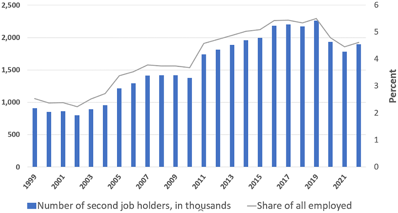
Multiple Job Holding in Germany: Absolute Numbers (left axis in thousands) and Employment Share (right axis in percentage) (1999–2022)
Central to this development was the 2003 expansion of the Minijob program (marginal employment, geringfügige Beschäftigung), which set strong incentives for taking up a Minijob alongside primary employment. Minijobs are small jobs that earn less than a monthly earnings ceiling (400 euros in 2006–07). Employees’ Minijob earnings are exempt from income taxes and social insurance contributions. Instead, employers pay contributions as fixed shares of gross earnings. Prior to the 2003 reform, Minijob subsidies could be used for only primary employment. Minijobs that were held as secondary jobs were subject to employee social insurance contributions of approximately 20% of earnings and to income taxes. After the 2003 reform, it became possible to benefit from the Minijob subsidy when Minijobs were held as secondary employment. Note that it was not allowed to split existing jobs or to hold two similar jobs with the same employer. The 2003 reform relaxed several additional restrictions: The Minijob earnings ceiling rose from 325 to 400 euros and an upper limit of 15 weekly hours of work was abolished. Also, the contribution rate for employers increased from 22% to 25% of Minijob earnings.
Employer contributions were increased again on July 1, 2006, from 25% to 30%. Figure 2 shows the number of Minijobs over time based on administrative data. It suggests that the reform substantially increased the incidence of MJH when regular employment was combined with a Minijob.
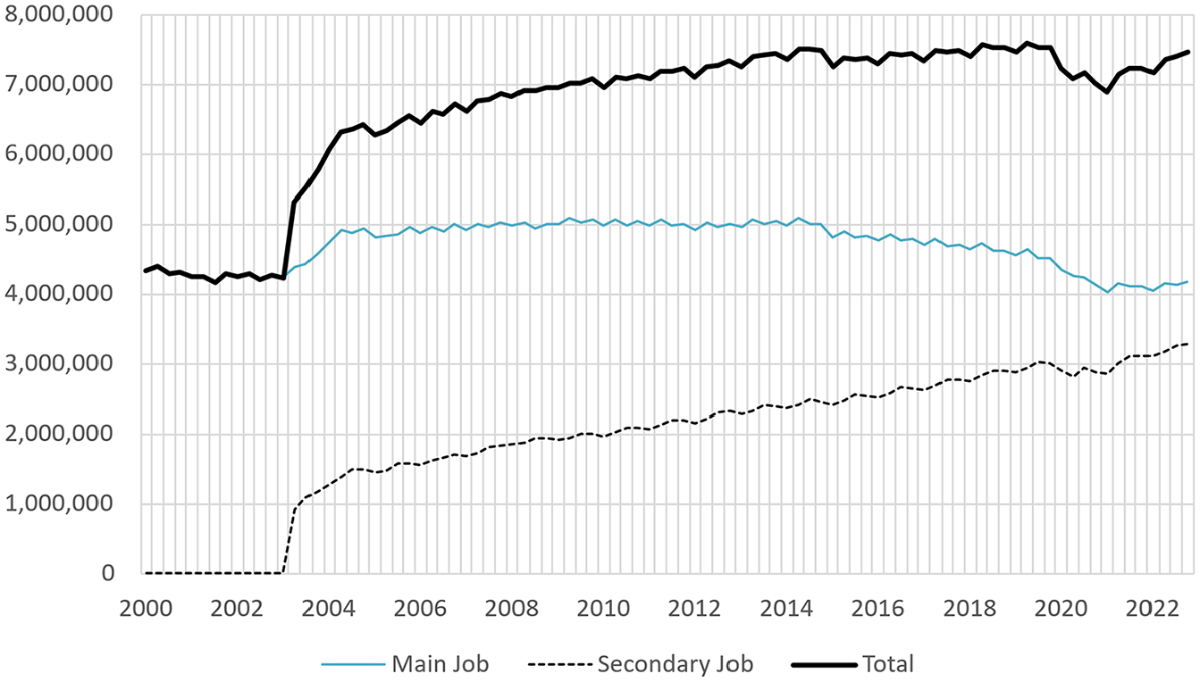
Minijob Employment: Main Job, Secondary Job, Total (Q1.2000–Q4.2023)
The fiscal burden generated by the subsidy for Minijobs as secondary jobs can be determined using a simple calculation. Employers of secondary job Minijobbers pay contributions of 30% (after July 2006) of Minijob earnings, which is 10 percentage points less than the regular joint social insurance contribution rate of 40% for employers and employees. Also, Minijob earnings are not taxed. In 2006, average income tax rates ranged between 0% and 40% depending on the individual situation. Thus, in 2006, the subsidization of secondary jobs based on social insurance rates plus income taxes implied lost public revenues of between 10% and 50% of secondary employment earnings. With approximately 1.5 million Minijobbers in secondary jobs in 2006 (see Figure 2) earning on average 300 euros per month, we obtain an annual subsidy of between 0.54 and 2.7 billion euros, ceteris paribus.
Motives of Multiple Job Holding
Literature on the determinants of and motivation for MJH rests on two main pillars: theoretical analyses (Shishko and Rostker 1976; Auray, Fuller, and Vandenbroucke 2020; Choe, Oaxaca, and Renna 2020; Lalé 2020; Lachowska, Mas, Saggio, and Woodbury 2022) and evidence from surveys that asked multiple job holders about their motivation (e.g., Wilensky 1963; Dickey, Watson, and Zangelidis 2011; Graf, Höhne, Mauss, and Schulze Buschoff 2019). Based on this evidence we can distinguish three main mechanisms acting as push or pull factors for MJH: investment and career motives, financial and liquidity motives, and psychological motives related to work–life balance or subjective fulfillment. 3 We briefly review all of these motives next.
The investment and career motive—also called the portfolio motive (Klinger and Weber 2020)—is central in the analyses of Panos et al. (2014). These authors emphasized the opportunity to use MJH to learn about alternative occupations and to obtain relevant training and work experience in preparation for subsequent career moves and occupational mobility. Working in heterogeneous jobs is interpreted as a human capital investment. The authors confirm that secondary job holders subsequently are much more likely than single job holders to move to self-employment or new primary employment. Also, secondary job holders are less likely to become unemployed or inactive. Panos et al. (2014) described two groups of multiple job holders; those who suffer financial constraints tend to work in the same occupation in the first and secondary jobs. By contrast, those who work in a different occupation in their secondary job are more likely to change their employer in the next period. This finding suggests that the latter benefit from human capital spillovers between first and second jobs and may advance their careers. Graf et al. (2019) confirmed these motivations based on answers to an online survey among 545 German secondary job holders: One-third of all respondents indicated that they hold secondary employment in order to widen occupational perspectives and expand their human capital, which clearly represents an investment motive.
If investment motives determine MJH, we can expect beneficial subsequent long-term career effects. In fact, we hypothesize first that those who enter secondary employment will benefit in the long run in terms of finding high-earning primary employment and increased annual earnings. Second, we expect that long-term developments are particularly beneficial if MJH is used to expand human capital, for example, by working in a variety of occupations and industries, or in more demanding jobs. In that case, MJH may be effective as a stepping stone to career advancement with non-transitory effects. Finally, MJH possibly offers a non-standard avenue to advancement, particularly for the labor market’s disadvantaged workers. One might imagine that disadvantaged individuals in the labor market, for instance, those with a low educational background or low initial earnings, have to show additional effort to signal their career orientation to employers. In that case, having multiple jobs may offer a mechanism or a bridge to career advancement.
The financial motivation was central to early economic analyses. Shishko and Rostker (1976) modeled the supply of secondary employment as a response to hours and thus earnings and liquidity constraints on a first job. Such constraints may be related to labor agreements, and they may derive from organizational restrictions at the firm level. In addition, workers might enter MJH in response to negative financial shocks, as an alternative to precautionary savings (Guariglia and Kim 2004), and as an insurance device in case of job insecurity and employment risk in primary jobs (e.g., Bell, Wright, and Hart 1997).
Finally, the psychological motivation related to work–life balance or subjective fulfillment typically shows up in surveys. Workers may derive utility from second jobs based on job heterogeneity, job amenities, or other benefits (see Heineck 2009). An example is an office worker who works as a musician at night. Here, working dissimilar jobs in primary and secondary employment is interpreted as consumption rather than investment. Overall, these motivating factors offer a foundation for the choice of conditioning variables in our methodological approach described in the Empirical Method section.
Data and Descriptive Evidence
Data
We use administrative data from the records of German unemployment insurance. The Sample of Integrated Labour Market Biographies (SIAB) offers a 2% random sample of all individuals registered with unemployment insurance between 1975 and 2017 (Antoni, Schmucker, Seth, and vom Berge 2019). 4 The SIAB data cover approximately 80% of the German workforce and exclude civil servants and the self-employed. We take advantage of precise information on the day-to-day employment status and earnings. The data provide a broad set of employment-related indicators 5 and offer a detailed profile of individual employment trajectories for large samples. This differs from survey data for which relatively small samples and short observation periods often limit long-term analyses (e.g., Conen and Stein 2021). The data structure allows us to track employment transitions and parallel employment periods with daily precision.
We are interested in the labor market outcomes after initiating MJH up to 10 years later, which can support the potential validity of an investment motive. Our sample entails workers who were employed full-time on June 30, 2005, did not experience spells of MJH in the five years prior to treatment, and were age 25–50 in 2005 (hence not likely to retire over the next 10 years). 6 We convert the data into an annual panel data set, using June 30 as the reference date (see Dauth and Eppelsheimer 2020).
Our treatment period runs from January 2006 to December 2007. We consider an observation to be treated as MJH if the individual takes up a second job within the treatment period and the employment spells overlap for at least 180 days (we modify this duration below). Observations with parallel employment periods in the same firms are not considered to be treated because we assume that these do not represent additional employment and likely reflect the coding of additional payments. For individuals who experienced treatment in 2006 and 2007, we consider 2007 and 2008 to be the first post-treatment year, respectively. We apply an event-time logic to reference post-treatment periods. The treatment definition as well as several outcomes rely on the differentiation between the main job and the secondary job. Following Klinger and Weber (2020), we define the highest-paying job as an individual’s main (or first or primary) job. For some multiple job holders, we have information on more than two parallel jobs; in these situations, we use only the information on the side job with the highest earnings in our analysis, which we consider for the entire spell, that is, at least 180 days. The control group consists of individuals who are full-time employed, age 25–50 on June 30, 2005, did not experience spells of MJH of more than 30 days in the five years prior to treatment, and do not take up secondary jobs of more than 180 days in the period 2006–2007. We condition our sample on being initially full-time employed in order to reduce the probability that MJH is a consequence of liquidity constraints and financial need. By considering only those individuals who originally held a full-time job it is more likely that any secondary job may represent an investment.
With these specifications, we obtain an unbalanced panel with 5,676 treated and 211,095 untreated observations, totaling 216,771 individuals. We follow these individuals annually for as long as 10 years after treatment. Treatment and control group observations leave the sample at similar rates: By year 10 after the treatment, 89% and 88% of the treated and control group observations are still in the sample, respectively (see Online Appendix Figure A.1 for annual rates). (Hereafter, Online Appendix material will be prefaced with only the “A.,” for example, Figure A.1, Figure A.2, Table A.1, Table A.2, and so forth.)
We consider six long-run labor market outcomes. We use log daily earnings for the main job and the overall annual labor market income as financial measures. 7 We use the probability of being in regular (full-time or part-time) employment and the probability of being in registered unemployment as indicators of the extensive margin of labor supply. We describe job mobility based on an indicator of year-to-year employer change. Additionally, we measure job mobility to high-paying employers by interacting the job mobility indicator with an indicator of whether the employer is in the top tercile of earnings firm fixed effects (AKM 8 effects, see Bellmann, Lochner, Seth, and Wolter 2020). All outcome indicators (except for annual labor market income) characterize the situation as of June 30 in any given year.
We apply entropy balancing (EB), which uses a wide set of covariates to derive weights that render control and treatment group observations comparable. Controlling for all covariates that potentially affect MJH and the outcomes, the procedure is similar to propensity score matching. The administrative data provide a variety of indicators that can capture the mechanisms determining MJH, as described earlier in the Motives of Multiple Job Holding section. We rely on economic theory, prior empirical research, and institutional information to justify our choice of indicators for EB. In particular, we consider indicators of individual demographic characteristics (gender, year of birth, educational degree, and federal state of residence), as well as detailed information on current and past individual employment (tenure, labor market experience, level of job complexity, and occupation). The biographical data allow us to describe past individual mobility in terms of changes of occupation or change of employer, for example. In addition, we use employer characteristics such as firm size, industry, and firm size changes over time. In total, these measures can capture mechanisms of financial, investment, and psychological motivation.
As this list of controls may overlook some relevant but unobservable factors, we follow the literature and add lagged dependent variables such as past earnings, employment, and unemployment to the set of predictors used in EB. The lagged measures go back for up to five years before treatment. Additionally, we consider higher-order polynomials and interaction terms between the listed variables. Table A.1 lists the control variables used in our entropy balancing.
Descriptive Evidence
Table 1 offers unweighted descriptive statistics on the characteristics of multiple job holders (treatment group, column (1)) compared with single job holders (control group, column (2)) in the treatment year. We find substantial differences between the two groups (see p values for mean equality tests in column (3)). Along with the description of the full sample, Table 1 offers a description of characteristics for the male (columns (4)–(6)) and female (columns (7)–(9)) subsamples, separately for single job holders and multiple job holders, with corresponding p values for tests of mean equality between those groups.
Descriptive Statistics
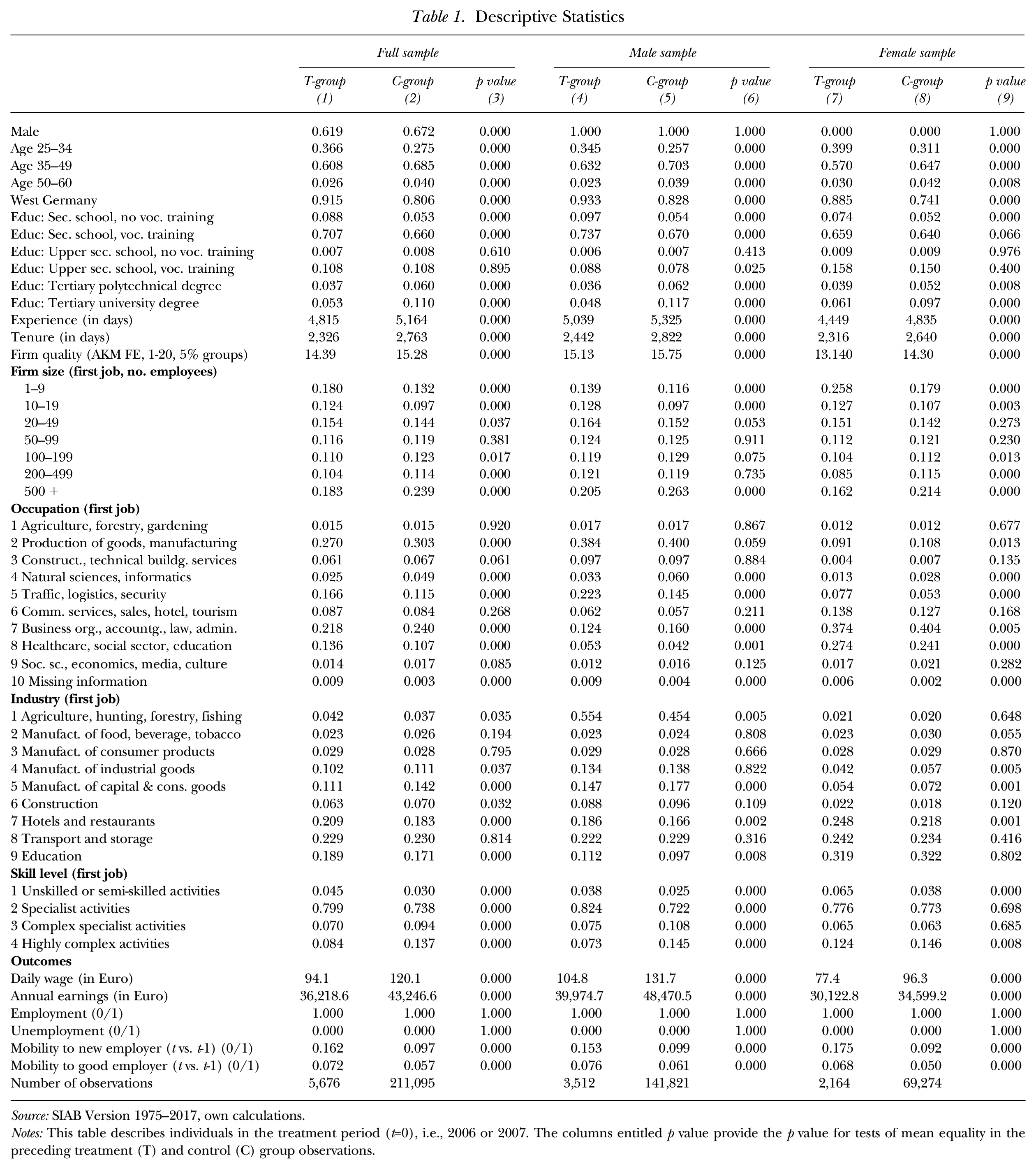
Source: SIAB Version 1975–2017, own calculations.
Notes: This table describes individuals in the treatment period (t=0), i.e., 2006 or 2007. The columns entitled p value provide the p value for tests of mean equality in the preceding treatment (T) and control (C) group observations.
Multiple job holders are younger, more likely to be female, and to live in West Germany. They are less likely than single job holders to hold a tertiary education degree, and they have accumulated less overall work experience and tenure. Also, the first job held in the treatment year differs somewhat between treatment and control groups: Multiple job holders work in lower-paying firms (based on mean percentiles in the distribution of AKM employer fixed effects) and in smaller firms. MJH is more likely in occupations such as “traffic, logistics, security” and “healthcare, social sector, education” and less likely in the “production of goods,”“business organization, accounting, law, administration.” While the industries of main job employment overall are rather similar for treatment and control group observations, multiple job holders are more likely to work in the service sector (e.g., hotels and restaurants) and less likely to work in manufacturing (e.g., manufacturing of capital goods). Multiple job holders are also less likely to be employed in highly skilled jobs. These characteristics agree well with those of the sample used by Tazhitdinova (2022).
In terms of outcomes in the treatment period, multiple job holders have substantially lower daily earnings in their first job and lower annual earnings from all jobs (see rows toward the bottom of Table 1). By construction, the employment and unemployment outcomes in the treatment period do not differ for the two groups. The probability of changing the employer relative to the year before is substantially greater among multiple than single job holders. The former are also more likely to change to a high-paying (labeled “good”) employer, which we consider as firms in the top third of the AKM fixed-effects distribution (Bellmann et al. 2020).
Most multiple job holders’ second job differs from the first job in terms of occupation and industry: 55.7% and 62.4% work in a different occupation and industry (at the 1-digit level as in Table 1), respectively. Our analysis is based on MJH of at least 180 days duration. Conditional on this restriction, the median time frame lasts 547 days (1.5 years) and the mean MJH lasts 1,019 days. Overall, in our sample, multiple job holding is a long-term activity. About 16% of secondary jobs are in the lowest qualification group, which compares to 4.5% and 3% of primary jobs in the treatment and control groups. Secondary jobs are concentrated in occupation groups comprising “traffic, logistics, security” (5) and “commercial services, sales, hotel, tourism” (6). Combined, only 25% (20%) of the primary jobs are in these occupations among the treatment (control) groups, although these occupations represent 46.5% of all secondary jobs.
Of 5,676 multiple job holdings, 92% combine full-time and Minijob employment at the time of treatment. An additional 5% combine part-time and Minijob employment. In our MJH sample, 92.6% of first jobs are full-time, 5.4% part-time, and 1.2% are Minijobs. Among secondary jobs the pattern is reversed, only 1.8% are full-time, 1.04% are part-time, and 96.1% are Minijobs.
Empirical Method
We are interested in the causal effect of an initial MJH episode on individual labor market outcomes in the long run. Given that no natural experiment assigns workers to MJH, the identification of the causal effect is challenging. We combine empirical strategies that control for observable and unobservable individual characteristics to account for potential self-selection into an initial MJH episode. 9 In step one, we use entropy balancing (EB) to derive weights to balance the observable characteristics of treatment and control groups prior to the treatment. In step two, we estimate fixed-effects regressions using weighted data. The fixed effects control for time-constant unobservable differences between individuals. When using pre-processed, matched data, the estimation in subsequent regression analysis is less sensitive to specification choices (Ho, Imai, King, and Stuart 2007) and may provide doubly robust estimators (Zhao and Percival 2017).
In our data pre-processing, we apply EB (Hainmueller 2012; Hainmueller and Xu 2013). Similar to propensity score weighting, EB derives a set of weights to satisfy pre-specified balancing requirements for treatment and control group observations. EB directly incorporates covariate balance in the weight function and does not require the process of propensity score modeling, matching, and balance checking (Hainmueller 2012). EB has gained popularity because of several advantages compared to traditional propensity score weighting: EB reduces imbalances more effectively, it can consider imbalances not only in first but also in higher order moments, and it is non-parametric and thus independent of functional form assumptions. 10
We need to balance the pre-treatment characteristics of those who did and did not initiate MJH. We use potential determinants of MJH as well as subsequent labor market outcomes in defining the set of balancing constraints. Based on the theoretical discussion above, we consider individual demographic characteristics that include variables describing a worker’s labor market biography in terms of employment, earnings, mobility, and information on past employers. Table A.1 provides more details on our set of matching variables. We use the first moments of these indicators and their lagged values as balancing constraints. EB yields weights based on which covariate distributions of the treatment and control group match on the specified moments. Under an assumption of conditional independence, a comparison of mean outcomes of the weighted treatment and control groups provides causal effects of the treatment.
The conditional independence assumption may not hold if unobservable individual characteristics are correlated with the treatment assignment and potential outcomes, for instance, if these are not fully accounted for by the weights from the data pre-processing step. To address this potential problem, we specify a regression model in our second step that accounts for individual-specific fixed effects. In particular, the following model on the weighted data can be used:

We consider different continuous and discrete outcome measures, Y, for each individual i in every observation year t. We control for individual- (θ i ) and event-year-specific (θ t ) fixed effects. The ε represents a random error term. The coefficient α gives the average treatment effect on the treated (ATT). In Equation (1), the ATT is modeled to be constant over time.
The central identifying assumption requires parallel paths in the development of the dependent variable in the absence of treatment, meaning that in the absence of the treatment the expected change in outcomes in the treatment group is identical to the expected change in the control group. With pre-processed data, this condition, as well as covariate balancing, are met mechanically in the pre-treatment period. We estimate the ATT as follows:
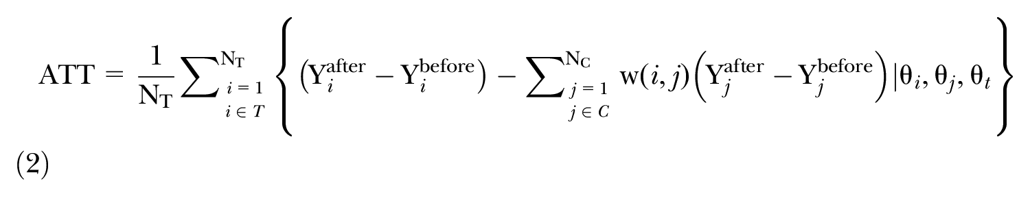
Here, T and C represent the groups of treated and control group observations, respectively. NT reflects the number of treated observations that experienced MJH. NC is the number of control group observations. And w(i,j) is the weight assigned to a control group observation j that is matched to a treatment group observation i. In Equation (2), Yafter and Ybefore are the average outcomes for each individual i or j from the treatment or control group, respectively. They are observed before or after the treatment. We use for each individual k:
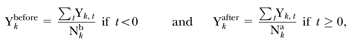
where

The indicator Postyear takes on the value 1 if t=s and 0 otherwise; here, the estimates of α capture potentially time-varying treatment effects between periods 1 and 10 after the treatment. Our empirical approach generates consistent estimates if the combination of EB and fixed-effects estimation, that is, weighting based on covariates and conditioning on person-specific fixed effects, accounts for observable and unobservable selection mechanisms. A remaining weakness of the approach is that we cannot account for time-varying unobservables. Nonetheless, we balance on past changes in employer size, which may account for expected downsizing including mass layoffs. In addition, we can claim external validity only to the extent that our observation window was not subject to specific calendar year effects. While the treatment period is not affected by institutional reforms, the long-run effects are measured in a period that includes the financial crisis of 2008–09. However, this crisis had rather limited effects on the German labor market (Burda and Hunt 2011); in addition, there is no a priori reason as to why it would affect the difference between treatment and control group outcomes. We use standard errors that are clustered at the individual level.
Results and Robustness
Baseline Results
The description of treatment and control group characteristics in Table 1 shows that the two groups differ in many respects. To account for these differences, we apply EB on the covariates listed in Table A.1. The balancing results can be inspected in Table 2, which presents a subset of covariate means and variances for the treatment and control group before and after balancing. A comparison across columns confirms that after balancing the weighted covariate, means are identical between control and treatment group observations.
Balancing Results on a Subset of Covariates
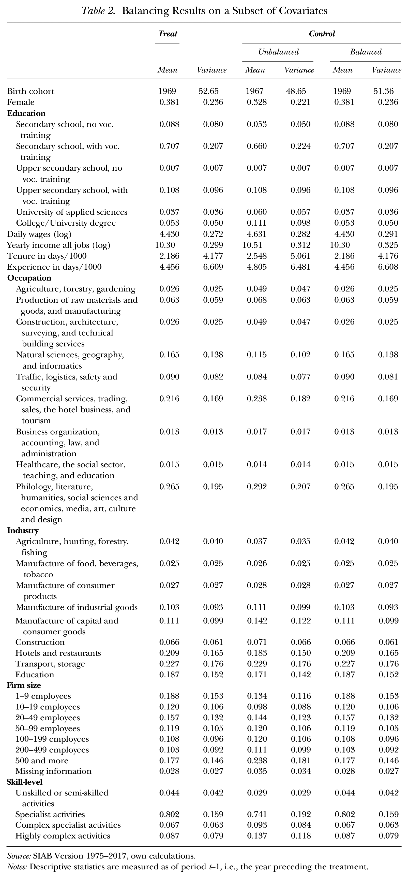
Source: SIAB Version 1975–2017, own calculations.
Notes: Descriptive statistics are measured as of period t–1, i.e., the year preceding the treatment.
We apply the thus pre-processed data to estimate Equation (3) in a fixed-effects difference-in-differences procedure. Figure 3 depicts the estimated coefficients αs before and after the treatment, and Table A.2 presents the coefficient estimates for the six labor market outcomes. 11 As expected, we observe no significant pre-treatment differences in the labor market outcomes of single vs. multiple job holders.
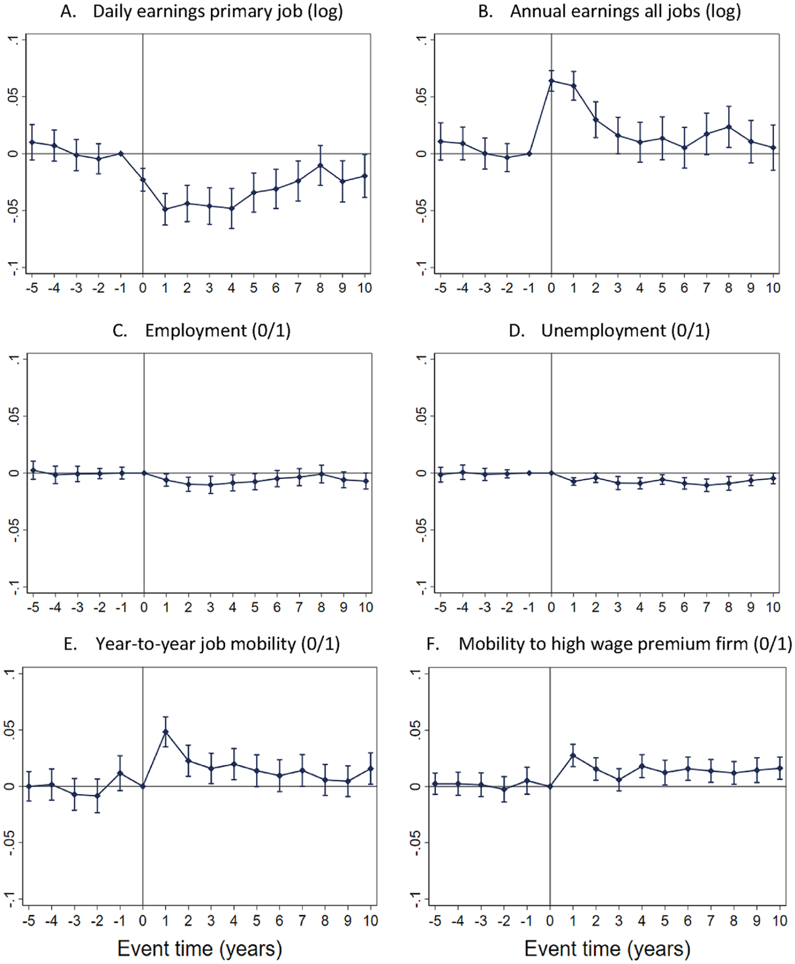
Baseline Estimation Results, Full Sample, 180-Day MJH Spells
Panels A and B of Figure 3 show the coefficients for our financial outcomes: individuals’ daily earnings in their main job and annual earnings from all jobs. Both cases use the period before the treatment (t = −1) as the reference period because later outcomes may already be affected by the treatment. We find that after the treatment, earnings from the main, that is, primary employment, decline significantly by approximately 5% more for multiple than for single job holders. We find this result to be surprising because a decline in primary employment earnings does not agree with either the investment motive, the financial motive, nor the psychological motive of MJH. To explain this result, we first investigate the relevance of the number of hours worked: the earnings decline drops to at most 2% when we condition on continued full-time employment (see Figure A.2). 12 In addition, it shows that multiple job holders are more likely to move to part-time employment as their main job (see Figure A.3). Interestingly, the treatment effect on daily wages in full-time employment is not significantly negative among workers who stay with their initial employer (see Figure A.2). This finding suggests that the drop in daily earnings is driven by switches to lower-paying jobs.
Panel B of Figure 3 shows that total annual earnings increase significantly more among multiple than single job holders in years 0–3 after treatment, which may reflect the additional income from secondary employment. In year 4, the overall earnings advantage drops and is no longer statistically significant. Overall, we find no long-run financial benefits of MJH; this can be attributable to a lack of changes in hourly wages, a change in hourly wages that is offset by the number of hours worked, or a change in the composition of jobs held simultaneously.
In panels C and D of Figure 3, we present the employment and unemployment outcomes after MJH. In both cases, the effects are small. The probability of full- or part-time employment and the probability of unemployment decline slightly but significantly after treatment. If this were the result of more frequent exits into self-employment after MJH, we would expect to see a higher propensity to leave the sample among treated observations because our data do not include the self-employed. 13 As discussed before, Figure A.1 does not support such a mechanism. Instead, the pattern of reduced employment and unemployment after an episode of MJH can be explained by an increased propensity among multiple job holders to take up a Minijob as their main employment (see Figure A.4).
Panels E and F of Figure 3 describe the impact of MJH on subsequent job mobility. In panel E we find significantly positive effects on overall job mobility through year 5 after the treatment. Panel F depicts the effects on mobility to high-wage firms. Again, we find persistent and significantly positive effects of 1 to 2 percentage points after the treatment. Relative to the pre-event mean transition probability of 5% to 7% for the treatment and control groups (see Table 1), this indicates a substantial effect of MJH.
Overall, the evidence with respect to the returns to MJH is mixed. On average and in the long run, no financial or employment benefits accrue from MJH. At the same time, individuals who took up secondary jobs subsequently changed employers more often and were more likely to take up employment in high-paying firms. On average, this last result, however, does not generate significantly higher main job wages. In additional estimations, we investigated the treatment effect on wage increases for those who continued to be full-time employed. The results (see Figure A.5) yield that in the first four years after treatment, the probability of a 5% or 10% wage increase is significantly higher among prior multiple job holders. So, while no financial benefits of MJH occur on average, a subgroup of multiple job holders did benefit from the experience. To better understand the heterogeneity of these findings, we now look into whether and how our findings differ across subgroups of the population.
Heterogeneity
We study two types of heterogeneities: those that directly address potential investment patterns of MJH and those that describe demographic groups. Within the first group, we consider situations of secondary job holding that differ in the extent to which the MJH experience might modify a worker’s human capital. In particular, we distinguish the effects of taking up a secondary job 1) in an occupation or 2) an industry that differs from that of the main job, and of taking up a secondary job 3) with higher skill requirements than the main job. In these situations, multiple job holders face more challenging demands connected to the secondary job and may add more to their human capital, compared to working in their main occupation, prior industry, and with similar skill requirements than in their primary job. Therefore, these may be the specific situations when individuals invest in the expectation of a potential future work environment.
Overall, our estimations do not yield significant returns to such investments: For those with different occupations and industries in their primary and secondary jobs, out of the six inspected labor market outcomes, we found only a somewhat higher job mobility in the longer run (see Figure A.6). The treatment effects did not differ significantly for the other labor market outcomes. In situations where the second job required higher skills than the first job, we found no significant differences in labor market outcomes.
Our second group of heterogeneity analyses focuses on various labor market outcomes after MJH by gender, education, and pre-treatment earnings. Table 1 shows gender differences in the patterns of MJH: On average, female multiple job holders are better educated, they work in smaller and typically less productive firms, and the distribution across occupation and industry groups differs substantially from that of male multiple job holders. While females’ primary jobs are mostly in education and the service sector, more than half of all male multiple job holders are employed in primary-sector industries. Given these heterogeneities, the long-run MJH effects may differ by gender.
We estimate our six models separately for men and women (see Tables A.3 and A.4 for gender-specific results). Figure A.7 shows the full results. While the estimates presented in rows (2) and (3) are similar for the two subsamples, the financial estimates depicted in row (1) differ more substantially. We observe significant, persistent negative effects of MJH on main job daily earnings of up to 7% for men. These effects are smaller for women and insignificant after period 3 (see panel A of Figure A.7 or panel A of Figure 4). Relatedly, men’s annual earnings significantly benefit from MJH for only two years whereas the relative earnings advantage for women persists in the long run (see panel B of Figure 4). In sum, we find no positive investment result of MJH for men whereas females’ annual earnings remain elevated in the long run after an episode of MJH.
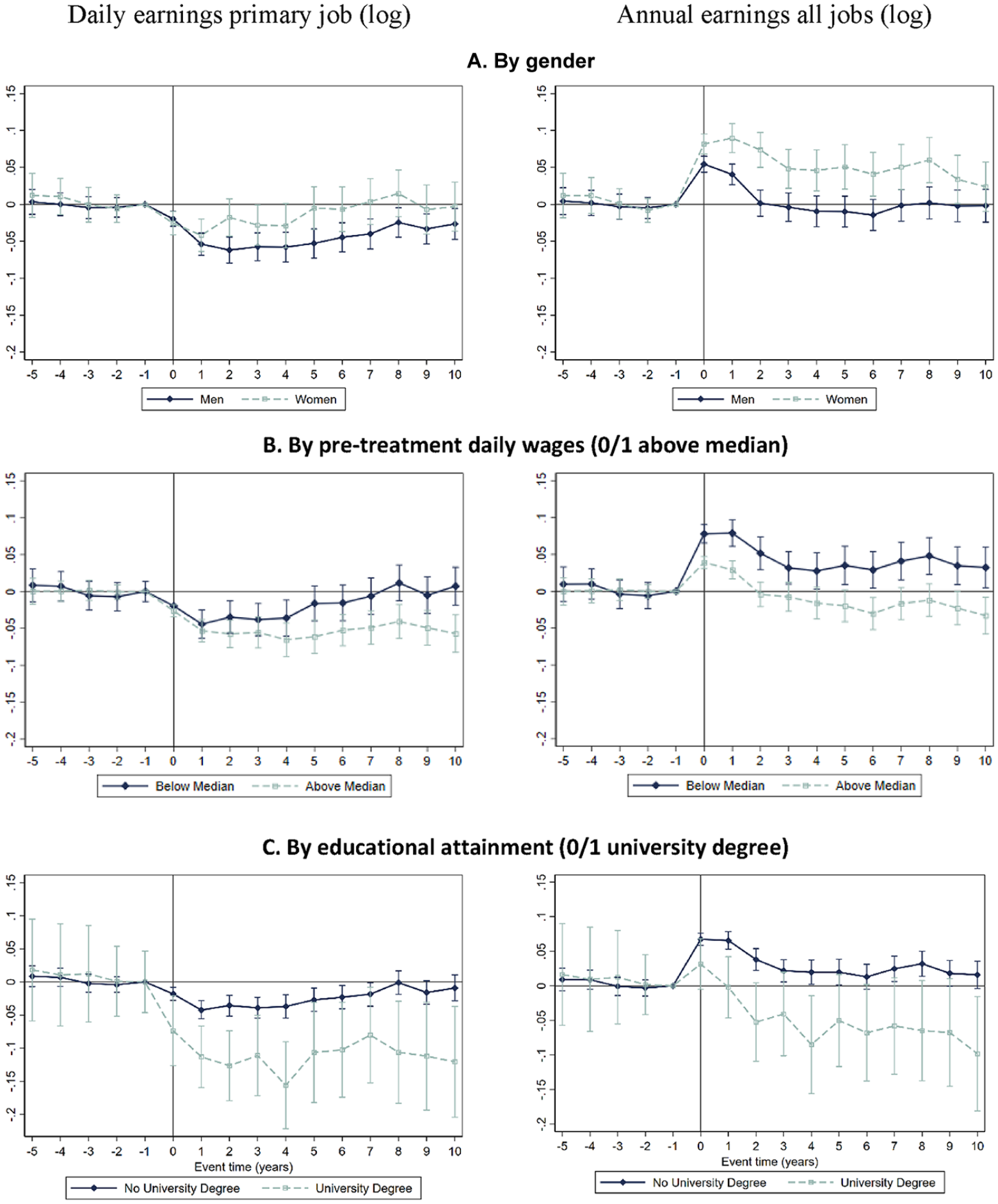
Heterogeneity of Treatment Effects on Daily Wages and Annual Earnings
In addition to heterogeneities by gender, we estimated separate models to learn about heterogeneities by pre-treatment wages and human capital. In the first case, we test whether the estimates differ for those with pre-treatment daily wages above vs. below the median. In the second case, we split the sample based on holding a tertiary degree prior to treatment. Similar to the results for male and female subsamples, in both cases we find few differences for the employment, unemployment, and mobility outcomes. In Figure 4 we show the financial effects for the groups: Panel B presents the heterogeneity patterns by pre-treatment daily wages and panel C presents the results for the subsamples with and without tertiary degrees. In both cases, we obtain surprising results. In panel A, the financial results of MJH are more beneficial for women than for men. Similarly, in panel B we see that those with lower pre-treatment earnings lose less in terms of daily wages and gain more in terms of annual earnings than those with higher pre-treatment earnings. The same pattern appears in panel C: The negative treatment effects of MJH on daily wages are smaller for those with low education, and the positive outcomes for annual earnings are larger for those with less education. Overall, these results suggest that beneficial investment outcomes of MJH are realized for those who were more disadvantaged before. This confirms the conclusion of the earlier Baseline Results section, based on which the average causal effect of MJH may obfuscate beneficial outcomes for subsamples. To learn more about the mechanisms behind the heterogeneous financial MJH effects by subgroups, we investigated earnings determinants and their development over time for different subsamples. This comparison yielded that certain subgroups’ initial disadvantages, for example, with respect to employer characteristics such as AKM fixed effects or firm size in period t–1, were equalized after the MJH treatment. For example, female multiple job holders worked for smaller-scale employers than did male multiple job holders before the treatment; however, the former worked for larger-scale employers than did male multiple job holders after the treatment. Also, the increase in employer firm size in the female sample is significantly larger among the treated than among the non-treated, which does not hold in the male sample. Overall, the additional labor market exposure of disadvantaged workers through MJH may contribute to balancing their initial disadvantages.
Robustness
We offer a broad range of robustness tests in four categories: 1) definition of the treatment group, 2) definition of the control group, 3) sampling rules, and 4) empirical procedure. Overall, the results do not seem to be sensitive to these modifications.
Our tests that adjust the treatment group definition focus on the required minimum duration of MJH spells. In our baseline setting, we consider an MJH treatment if different jobs overlap for at least 180 days. We chose this rather long period because a minimum exposure may be necessary to realize investments in additional human capital and new networks. This minimum overlap requirement differs from choices in the literature using survey data: These studies define an MJH event if the individual states they “currently” hold more than one paid employment (see, e.g., Panos et al. 2014; Conen and Stein 2021). Also, Felder (2019), who worked with administrative data, uses this definition. Tazhitdinova (2022) also worked with German administrative data and required an overlap of at least a 15-day duration in her analyses. To determine whether our definition of the treatment affects our results, we generated new samples using minimum MJH durations of 30 and 360 instead of 180 days. We show the estimation results using these samples in Tables A.5 and A.6. Comparing the results to those presented in Table A.2 we find the treatment effects to be robust in terms of sign, magnitude, and statistical significance. 14
We pursued two robustness tests that redefine the control group. First, we omitted all observations from the control group that were themselves treated by MJH of at least 180 days duration in later years. Second, we dropped all observations from the control group that in 2006 and 2007 experienced MJH times that were too short to fall under the treatment definition of between 30 and 180 days. The number of control group observations dropped from 211,095 to 193,818 or by 8.7% in the first case and to 298,836 or by 1.1% in the second case. Tables A.7 and A.8 show the estimation results. We find that the changed definitions do not modify our conclusions from the baseline analyses.
Our third category of tests modifies the overall sampling rules. We start by changing from an unbalanced to a balanced sample, in which we require that all observations are observed at least in the periods t− 2 to t + 10. This approach might affect our results if treatment and control group observations differ in their propensity to leave the sample. Table A.9 presents the estimation results on this subsample. They hardly differ from our baseline findings.
In our data description, we pointed out that 90% of our multiple job holders combine full-time and Minijob employment. To determine whether this group differs from others, we re-estimated our models for those 5,109 observations that combine full-time and Minijob employment. Table A.10 shows that the results are very similar to the baseline results in Table A.2.
A final test in this set is motivated by the recent literature on the heterogeneity of difference-in-differences estimation results over time (e.g., Goodman-Bacon 2021; de Chaisemartin and D’Haultfoeuille 2023). To test for heterogeneous treatment effects over time, we estimated our models using only those treatments that occurred in the first of the two considered treatment years. This reduces the number of observed MJH treatments from 5,676 to 2,886. Nevertheless, the results are very similar to our baseline findings (see Table A.11).
The final category of robustness checks modifies our estimation approach. We expanded our set of conditioning variables in the derivation of the EB weights to include the so-called AKM firm fixed effects (Bellmann et al. 2020). These effects are available and thus applied for the years 1998–2004 in the pre-treatment period. By balancing firm characteristics, in addition to firm size and its lagged values, we make employees comparable across firms; this addresses the concern that individuals may anticipate negative firm shocks. Table A.12 presents the estimation results that confirm the results in Table A.2. 15 Finally, we applied a propensity score–based estimation approach. The estimation results in Table A.13 confirm our findings.
Conclusions
This study is the first to investigate long-run career outcomes of multiple job holding (MJH). It seems plausible that MJH can enhance work experience and human capital, generate human capital spillovers between first and second jobs, and strengthen labor market networks. We investigate whether the long-run labor market outcomes after MJH offer evidence of successful investments or generate only transitory benefits.
Our analysis takes advantage of large samples, precise information, and long-running data from administrative sources. We apply a doubly robust estimator to account for selection on observables into MJH using entropy balancing (EB); individual treatment and control group observations are balanced in terms of pre-treatment characteristics. We then apply the pre-processed data in a difference-in-differences setting that accounts for person-specific time-constant fixed effects. This estimation procedure allows us to estimate causal effects under relatively mild identifying assumptions.
Overall and on average, there are neither positive MJH effects on annual earnings nor on employment outcomes. We find that those who enter secondary jobs subsequently earn less in their primary employment compared to matched control group observations who did not hold additional jobs. This relative earnings disadvantage in the main job is connected to a reduction in the number of hours worked and employer changes. At the same time, overall annual earnings, including income from additional jobs, are significantly higher for multiple job holders for a short period of about three years after starting MJH; this suggests that multiple job holders divide their working hours between the different jobs. MJH slightly reduces the propensity to be in regular employment and the risk of unemployment; instead, we see a significantly increased probability of choosing Minijob employment as a primary job. Those who initiated MJH are more likely to change employers and move to a high-paying employer than are single job holders in the control group.
We investigate whether beneficial labor market outcomes are tied to specific secondary job choices, such as working in a different occupation or industry compared to the first job or taking up higher qualified work in the secondary job. We do not find confirmation for such patterns. Interestingly, we observe that disadvantaged groups in the labor market, such as females, those with relatively low pre-treatment earnings, or those with less than tertiary education, benefited significantly more from MJH than did the other groups. We find that these groups’ earnings determinants increased more strongly after the treatment than the earnings determinants of their non-disadvantaged counterparts. Therefore, MJH may have opened up opportunities in those precarious segments of the labor market where individuals are likely to get stuck in their primary careers or to hit glass ceilings.
We offer a broad set of robustness checks, changing the definitions of treatment and control groups, and changing the sample specifications or the empirical procedures. Our results stand up to these modifications. Although the strength of our study is its long-term perspective, which is new to the literature, we are also aware of two limitations of our contribution. First, the MJH situation in Germany is affected by the institutional framework of Minijob employment. Being tax-free and exempt from social insurance contributions, this framework for MJH may be similar to informal work arrangements but it differs from labor markets in which secondary jobs are strictly regulated. This institutional background may affect the selection into MJH, which in Germany is less pronounced among the higher educated than in other countries. Therefore, our findings of heterogeneous outcomes for disadvantaged and non-disadvantaged MJH workers may be particularly relevant. If the disadvantaged are more likely to be in MJH only in Germany, then the lack of long-run effects for the other group may be the most relevant takeaway message for MJH in other labor markets. Finally, a limitation of our data is that we cannot separately identify causal effects on hourly wages and the number of hours worked.
Given the increasing prevalence of MJH in many industrialized countries, it is important to understand its long-term outcomes. For Germany, where small secondary jobs are generously subsidized, we cannot confirm general positive returns to MJH. This finding is relevant for the optimal design of labor market and social insurance policies for workers in the gig economy and deserves attention in other labor markets as well.
Supplemental Material
sj-pdf-1-ilr-10.1177_00197939251361359 – Supplemental material for Long-Run Career Outcomes of Multiple Job Holding
Supplemental material, sj-pdf-1-ilr-10.1177_00197939251361359 for Long-Run Career Outcomes of Multiple Job Holding by Johanna Muffert and Regina T. Riphahn in ILR Review
Footnotes
Acknowledgements
We are grateful to Matthias Collischon, Anna Herget, Irakli Sauer, Erwin Winkler, Michael Oberfichtner, and the participants of the 2023 meeting of the Verein für Socialpolitik’s standing committee for social policy, the FAU LASER 2023 annual meeting, the IAAEU seminar in Trier 2023, the 2023 Colloquium on Personnel Economics (COPE), as well as the 2022 ESPE and EALE annual conferences for helpful comments.
Additional data-related information and copies of the computer programs used to generate the results presented in the article are available from
1
2
For ease of understanding, we refer to firms instead of establishments; however, all firm indicators provided by the Institute for Employment Research (IAB) are measured at the establishment level.
3
Campion, Caza, and Moss (2020, table 4) illustrated the three categories. As a motivation underlying the finance category, they list the desire to avoid hours constraints, pay off debts, meet regular expenses, insure against job insecurity, buy something special, or save for the future. For the career development category, they list an interest in heterogeneous jobs, the opportunity to learn, and work shifts of the primary job. For the psychological fulfillment category, the relevant motivations are to enjoy work, expression of identity, the desire to mix with other people, and to balance the primary job experience, work–life balance, and flexibility.
4
We use the weakly anonymized version of the SIAB 1975-2017 (DOI: 10.5164/IAB.SIAB7517 .de.en.v1). Data access was provided via remote data access and on-site use at the Research Data Centre (FDZ) of the German Federal Employment Agency (BA) at the Institute for Employment Research (IAB).
5
This includes occupation, job requirements, tenure, daily wages, and type of employment (i.e., full-time, part-time, or marginal). At the individual level, we know age, gender, federal state of residence, and education. The information on the highest level of education is reported by the employer and is missing or inconsistent in many cases (Dauth and Eppelsheimer 2020). We use the imputed version provided by the FDZ, which relies on the imputation procedure by Fitzenberger, Osikominu, and Völter (2006). At the employer level we observe, for example, firm size, worker characteristics, region, and industry.
6
We choose the year 2005 as a starting point to circumvent any immediate responses to the reforms introduced in April 2003. The German welfare system was reformed starting January 1, 2005. However, as we condition on full-time employment on June 30, 2005, the latter reform should not affect the observations and processes of interest here. We exclude all observations from the treatment and control groups who experienced MJH for at least a 30-day duration before our observation window. We generally do not consider shorter spells of overlapping jobs as MJH because periods shorter than one month may include job transitions. We condition our samples to be in full-time employment to establish comparability; allowing part-time workers would introduce substantial heterogeneity of starting conditions.
7
8
AKM refers to John Abowd, Francis Kramarz, and David Margolis. 1999. High wage workers and high wage firms. Econometrica 67(2):251–333.
9
We exclude observations with MJH work prior to our treatment period in order to circumvent staggered treatment assignments. We code treatment exposure to initial treatment as a permanent individual feature, which avoids issues of dynamic treatment assignment and multiple treatment periods (see, e.g., ![]() ).
).
10
Ruhose, Thomsen, and Weilage (2019) and Lergetporer, Ruhose, and Simon (2018) used similar methods in a panel data setting. For additional examples of prior applications, see Marcus (2013), Anger, Camehl, and Peter (2017), Bossler and Gerner (2020), Jones, Rice, and Zantomio (2020), and/or ![]() .
.
11
We also considered a model that additionally controls for time-varying indicators of the federal state of residence and industry of main employment. These controls do not affect the effects of interest. To avoid potential endogeneity issues, we base our discussion on specifications without covariates.
12
Our data do not provide information on working hours or overtime work. Employers provide information on whether employment is full- or part-time. Because this information is not relevant for administrative purposes, however, it is considered to not be fully reliable.
13
Using survey data from the German Socioeconomic Panel, we found that between 2002 and 2016, only 2.7% of those who started MJH in period t–1 and were not self-employed at that time subsequently shifted to self-employment. This supports the conclusion that self-employment is not a major phenomenon in our setting.
14
We ran an additional robustness test changing the treatment group: To separately consider the effect of only an initial MJH spell, we omit all treated observations that re-enter MJH episodes after period t+2. The results do not differ substantially from the baseline.
15
In addition, we inspected the weights of the control group observations generated by EB to ensure that no influential observations occur. The observation with the highest weight of 0.108 accounts for 0.002% of the sum of all weights, which is very small and suggests that we do not have concentrated weights. Estimation results are robust to omitting this control group observation.
References
Supplementary Material
Please find the following supplemental material available below.
For Open Access articles published under a Creative Commons License, all supplemental material carries the same license as the article it is associated with.
For non-Open Access articles published, all supplemental material carries a non-exclusive license, and permission requests for re-use of supplemental material or any part of supplemental material shall be sent directly to the copyright owner as specified in the copyright notice associated with the article.