
Abstract
This study attempts to analyse the relation of ecological footprint (EF) and air pollutants—CO2, N2O, SO2 and CH4—with economic growth, urbanisation, foreign direct investment and energy consumption through environmental Kuznets curve (EKC) framework by employing fixed/random effect model. It involves a panel of 55 selected countries from several income groups—high, middle and low—covering the period 1990–2018. A theoretical approach has been developed to analyse the pollution intensity of population, based on decomposition analysis coherent with application of the notion of Kaya identity. The results confirmed the existence of inverted U-shaped relationship for EF and SO2 in all types of countries. The pollutants—CO2, N2O and CH4—exhibit inverse U-shaped EKC in middle- and low-income countries. Only for high-income countries, N2O model detects the existence of U-shaped curve. The study suggests that reconsideration of some economic and environmental policies is necessary to mitigate environmental degradation issues.
Introduction
The recent concern of sustainable development is mostly related to how to maintain environmental quality. The key challenging issue of natural scientists is to overcome the harmful effect of climate change and recover the natural resource misused arbitrarily in the name of higher growth in developed nations and developing economies. Researchers generally want to figure out whether or not environment degrades with the rise in income up to a certain turning point, after which there occurs decline in environmental pressure. For this purpose, they try to capture the interaction between environmental degradation and economic development by the environmental Kuznets curve (EKC) framework. At present, it is one of the major concerns how to balance between economic development and conservation of environment in the global economy. Among several measures of environmental degradation, the most comprehensive measure is considered here, that is, ecological footprint (EF). There are some studies (Babbou et al., 2017; Omri et al., 2015; Wackernagel et al, 1999) that have considered EF as a proxy indicator for environmental degradation. According to them, while CO2 emission accounts for partial atmospheric dynamics, EF envelops the entire biosphere and hence provides an inclusive aspect of viewing environmental deterioration better than other forms. The EF measures the impact of anthropogenic activities for productive areas (croplands and grazing lands) forested to produce wood products, marine areas for fisheries, built up land for housing and infrastructure, and forested land to absorb CO2 emission from energy consumption (Ewing et al., 2010). These amounts of land and water body produce biological product to meet human needs and mitigate accompanied waste (Wackernagel et al., 2002). According to Solarin et al. (2018), it is considered as an integral indicator for considering depletion of environmental resources. Additionally, human activities like consumption patterns, food habits and environmental indifference and so on not only exhaust the long-term stock of available resources but also spoil the biosphere. So, based on these studies, EF may be considered as similar to environmental degradation.
Further, it may be noted that CO2 emission represents only a part of greenhouse gases (GHGs) contributing to total environmental degradation captured in EF. To control global warming, ‘United Nations Framework Convention on Climate Change’ targets mainly four GHGs, that is, CO2, CH4, N2O and SF6. CO2 is the largest contributor to polluted atmosphere and majority of the studies are based on carbon-growth nexus through EKC framework. Among the non-CO2 GHGs, CH4 is the most powerful pollutant followed by N2O in climate change issues. SO2 emission which results from the fast growth of industrialisation had been the earlier matter of concern among the GHG issues. Different surveys (Pasten et al., 2012; Stern, 2004) revealed that at the initial stages, higher economic development generates huge pollution and after a particular level of income it becomes capable to reduce the amount of pollution. The aspects of EF and emission of GHG gases as a measurement of environmental degradation were considered together in very few studies, for example, Saleem et al. (2019). They find out the role of human capital and bio-capacity on environmental quality involving EF and GHGs-CO2, N2O and CH4. But the impact of economic variables on EF and four GHG gases together has hardly been considered across different income group countries. In view of the current concern about worldwide climate change, it seems imperative to undertake a study with the following specific objectives.
To find out the impact of GDP and other variables like population, foreign direct investment (FDI), fossil fuel energy consumption and renewable energy consumption on variation in EF, CO2, N2O, SO2 and CH4 in different income group countries. To build a decomposition model to analyse the pollution intensity of population, based on Kaya identity. Some sound environmental policies are to be served for sustainable future and abating pollution.
Literature Review
Many researches on theoretical and empirical study have been focused on EKC estimation for individual countries or groups involving different periods. Researchers have used different proxy variables of economic growth, climate change, resource use, financial investment and so on.
The initial categories of literature are based on the EKC relationship between resource degradation and economic growth. Bulut (2020) used EF as an environmental destruction indicator and the control variables as FDI, renewable energy consumption and industrialisation. He confirmed that EKC hypothesis prevails in Turkey from 1970 to 2016. Using autoregressive distributed lag model, Hassan et al. (2019) investigated the long-run relationship and the effect of natural resource and economic growth on ecology in Pakistan. The result supports the EKC hypothesis and bi-directional causality between EF and natural resources. Considering EF as a proxy of environment degradation, Dogan et al. (2020) investigated the EKC hypothesis validity for BRICS countries covering the time 1980–2014. Some of the previous works of literature (Abdouli et al., 2017; Bese, 2018) focused on the fact that CO2 is the chief contributor to climate change and energy consumption plays a significant repercussion on CO2 emission at the national or global level. From the work of Aye and Edoja (2017), it is revealed that economic growth negatively affected CO2 emission in lower growth regimes, but the opposite happened in higher growth regimes. The result indicates a ‘U’-shaped relationship between economic growth and CO2 emission. We have also focused on some literature on EKC involving non-CO2 GHG emission as N2O, SO2 and CH4. In Germany for the time from 1970 to 2012, Monserrate and Fernandez (2017) evaluate the relationship between N2O, GDP, agricultural land use and export by using the autoregressive distributed lag (ARDL) model. The result confirms the quadratic long-run relationship and existence of EKC. Manuel and Mario (2017) confirmed a quadratic EKC relationship between N2O emissions and economic growth in Germany. Khan et al. (2016) confirmed the U-shaped relationship of perfluorocarbon emission and particulate matter-2.5 micrometre emissions with the per capita income in some selected developed countries. Based on the time series data, Anastacio (2018) found evidence of U-shaped EKC for CH4 in case of Argentina. Fosten et al. (2012) got significant evidence of inverse U-shaped EKC for the components of emissions, CO2 per capita and SO2 per capita in United Kingdom. In United States for the period 1990–2012, Polemis and Stengos (2018) found that economic growth plays a significant role in emission of SO2 and NOx.
Thus, we see that various researches have extensively tried to re-investigate the EKC relationship of environmental factors with economic growth issues. However, the upshot of increase in EF and GHG pollutants, namely CO2, N2O, SO2 and CH4 emission, together for different income group countries have been considered less often. Besides these, here the impact of control economic variables such as foreign investment, urban population growth, fossil fuel and renewable energy consumption is also verified.
Data Source and Key Variables
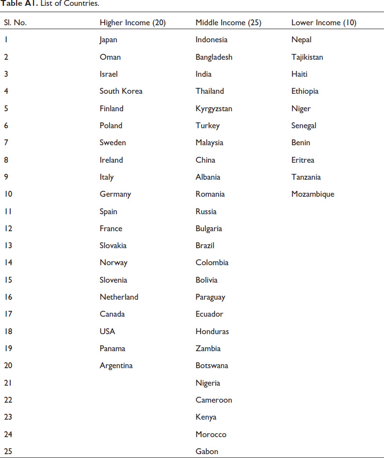
This study uses a panel framework with 55 countries over the time period 1990–2018. World Bank classifies all the countries into different income groups, that is, high, middle and low (Figure 1) and all the countries have distinct concentration of EF, air pollutant, financial investment measurement, urbanisation trend and energy consumption profile. Further, the country selection in each income group has been done based on data availability as well as some features of similarity. According to some authors, geography plays a crucial role in economic development processes (Bosker & Garretsen, 2012; Gallup et al., 1999). There is evidence that consumption patterns associated with geography can directly influence environmental degradation (Bednar & Sarapatka, 2018; Zhou et al., 2019). So, the role of geographical factors on environmental degradation is captured by selecting the countries from four continents, Asia, America, Europe and Africa, keeping in mind variation in income and consumption pattern. We have considered 20 countries from higher-income group, 25 countries from middle-income group and 10 countries from lower-income group covering four continents (Table A1).
Map of the Study Area Using Arc-GIS.
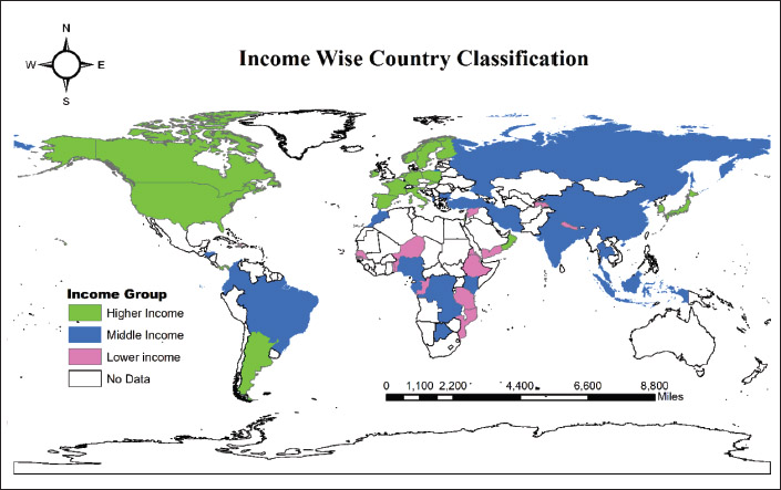
Map of the Study Area Using Arc-GIS.
Besides, EF, CO2, N2O, SO2 and CH4 are the different greenhouse gases that are considered as climate change factors. Further, FDI, urban population growth and energy consumption are considered as control variables impacting on environmental degradation and climate change issues. The data are sourced from Global Ecological Footprint, Emission Database for Global Atmospheric Research and World Bank Development Indicator.
The key variables are explained as follows:
An Aspect of Environmental Degradation, Pollution and Cross-Country Variation with GDP: EKC Framework
With the passage of time, the EKC hypothesis has been transformed into cubic versions which show the possibility of somewhat modified version of EKC hypothesis in terms of N-shaped relationship. However, for different income group countries, this requires a very long time series to verify its possibility. In this study, however, due to relatively smaller time series, possibility of inverse U-shaped relation is considered by using the following two models:
Model 1: Environmental Degradation Model

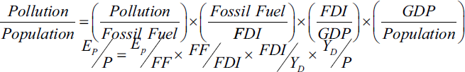
Model 2: Pollution Model


where ‘j’ indicates the countries and ‘t’ indicates the time period from 1990 to 2018.
α indicates the slope of the coefficients of the corresponding variables. Depending on the β coefficients related to GDP per capita, the EKC will adopt different shapes.
In case βi1 = βi2 = 0, we have no relation between the economic growth and pollutant. We get horizontal shape or flat pattern of the curve as depicted in graph (a) in Figure 2.
Relation Between Environmental Degradation and GDP Per Capita.
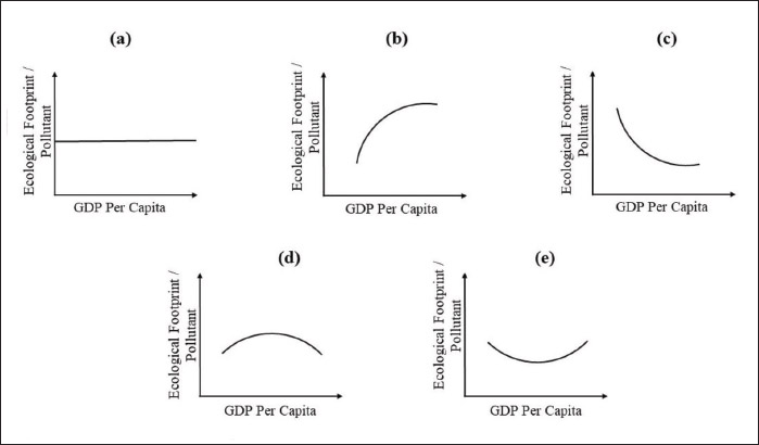
If βi1 > 0 and βi2 = 0, there will be a monotonically increasing relationship such that dependent variable increases along with income growth. This gives rise to graph (b) in Figure 2.
If βi1 < 0 and βi2 = 0, the pollutant/environmental degradation monotonically decreases with GDP. This is expressed in graph (c) in Figure 2.
If βi1 > 0 and βi2 < 0, we get the inverted U-shaped EKC. Usually, at the initial stage, pollution increases and after a certain income level it falls. This is shown in graph (d) in Figure 2.
If βi1 < 0 and βi2 > 0, we get a U-shaped relationship, as reflected in Graph (e) in Figure 2. This is an unusual case when pollutant falls with GDP in the initial years and after a certain point of time pollution increases. Here, i = 1, …. 5.
Apart from this, the possibility of an N-shape curve is reflected in an equation with a cubic power of GDP. It indicates that after certain time lapse, the pollution/environmental degradation again rises alongside GDP. However, this is usually reflected in a longer time series data. For instance, Boluk and Mert (2015) estimated a cubic relation for CO2 and GDP considering data for Turkey over the period 1961–2010. Zhang (2021) carried out testing of N-shaped curve for CO2 in case of China by considering the annual time series dataset from 1971 to 2014. In the present analysis, the time period covers 1990–2018, that is, 29 years and this period may be too short to reflect N-type EKC in some countries for some of the pollutants.
The existence of EKC across the countries has been measured by panel regression and we have considered suitability of fixed effect/random effect model based on the Hausman test. Significant probability value of the Hausman test implies that fixed effect is appropriate.
Elasticity Approach to the Notion of EKC
In order to reconcile these aspects with the observed patterns of EKC, some decomposition of pollution intensity of population is carried out with subsequent analysis and exposition in terms of some derived elasticity coefficients.
Taking log in both sides,

Taking first difference,

Or
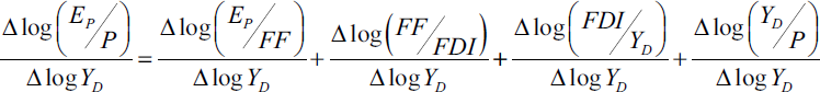
Or
Where,
The ratio PIP measures the total emissions/effluents related to overall population of the economy. Since pollution is influenced by fossil fuel energy consumption which is assumed to be the main ingredient of any kind of production and transportation of these products,
€PIFF indicates elasticity of pollution intensity of fossil fuel energy use with respect to GDP. In case of developed countries, this value is likely to be negative as opposed to positive in case of developing low/middle-income countries. This is because with rise in GDP in advanced countries, there occurs the tendency to shift to fuel-efficient renewable sources of energy. Furthermore, with increasing output, developed countries gradually take resort to diverse economic instruments like tradable pollution permits, emission tax, carbon banks and so on that help regulate the use of fossil fuel together with increasing responsiveness of people. The developing countries lag behind such adoption because of relatively high cost of advanced technology to switch to green energy and apathy of people to respond to the regulatory measures. Besides this, the developed countries spend huge amount towards devising fuel-efficient green energy, in the face of intensive programme of industrialisation triggered by the flow of FDI. This is evident from the fact that vast expanse of land is being allocated in developed countries for cultivation of biodiesel like ‘jatropha’. This may lead to a negative value for the elasticity of FFFDI with respect to GDP (
The results corresponding to the mentioned models of EKC for each income group country are separately given in Tables 1–6.
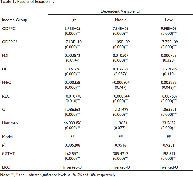
Results of Equation 1.
Results of Equation 1.
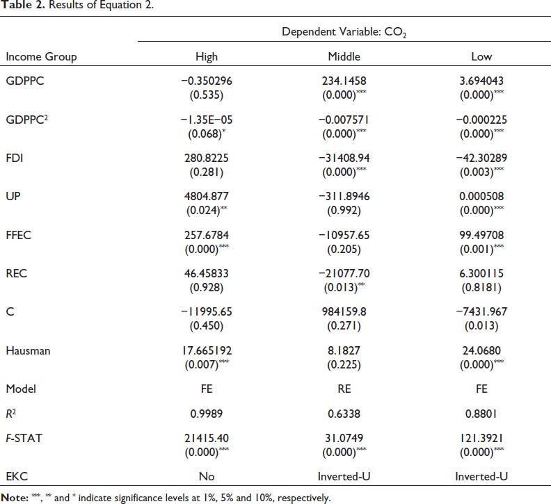
Results of Equation 2.
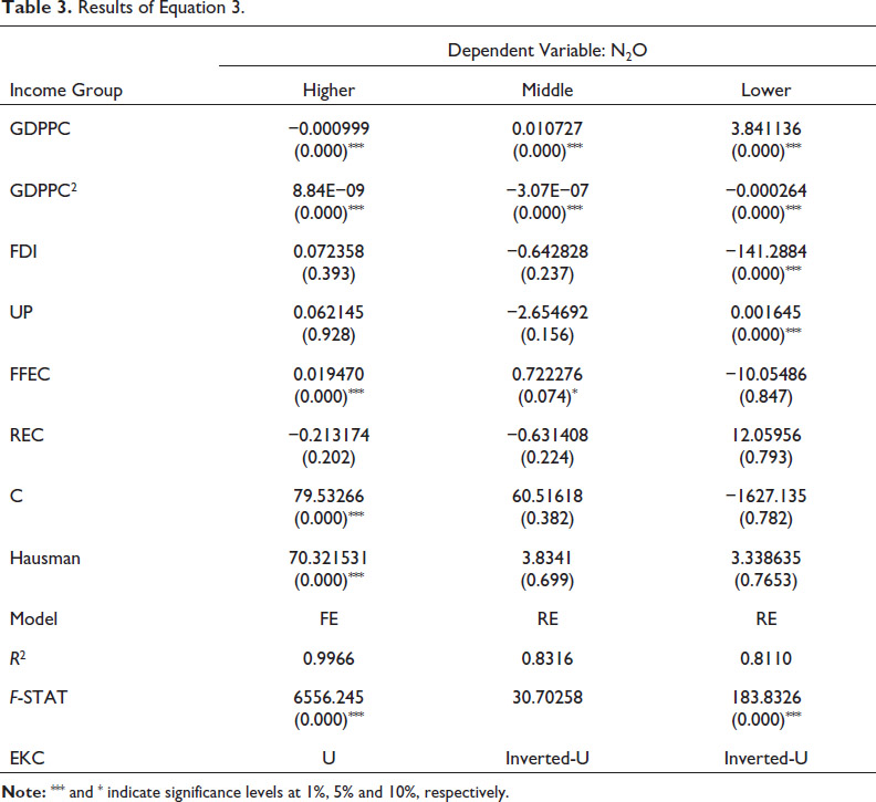
Results of Equation 3.
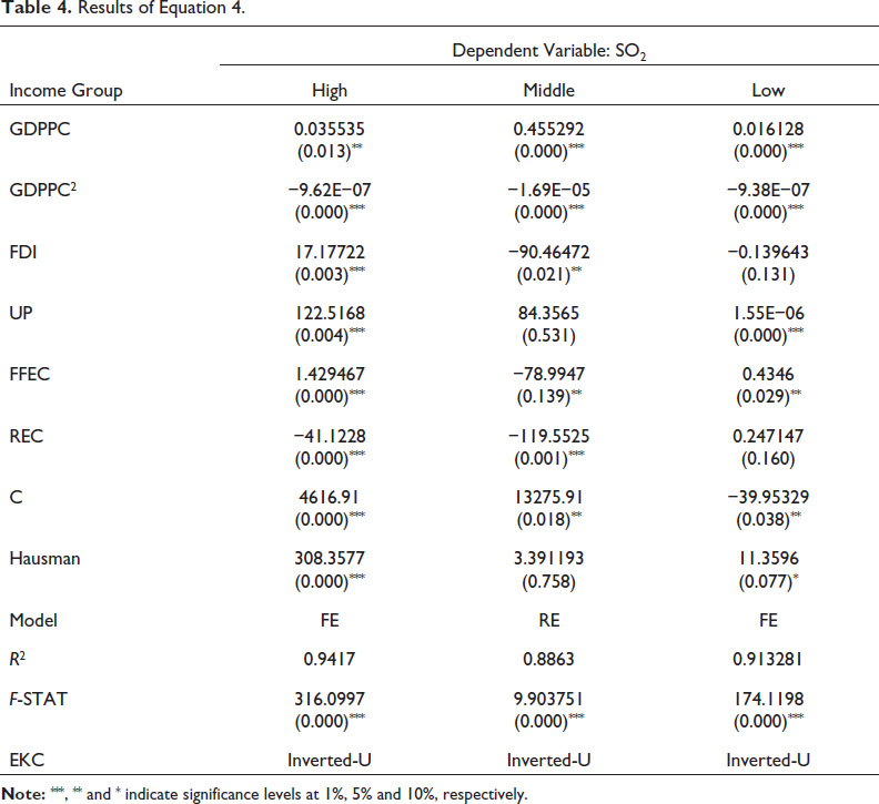
Results of Equation 4.
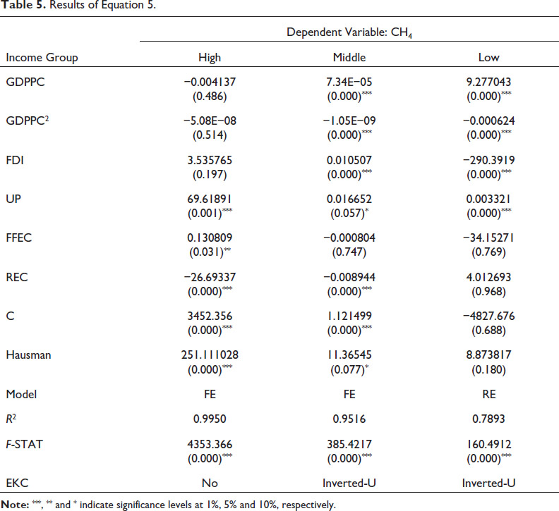
Results of Equation 5.
Country Group and Degradation-wise EKC Pattern.
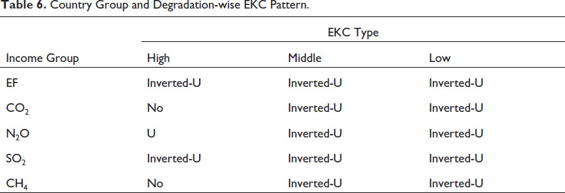
Table 1 shows the result of environmental degradation model. In case of EF, the result of the Hausman test shows the suitability of fixed effect model in all-income group countries. The estimated results reveal inverted U-shaped relationship between EF and income. The result also indicates R2 value as 0.88, 0.95 and 0.92 for the respective country groups. As expected, FDI has positive significant impact on the status of the EF in these groups of countries excepting low-income group. It usually happens due to the fact that FDI influences the domestic industrial production and value-added in wholesale, which enhances the overconsumption practice in human nature. Further, FDI has an impact on transportation, various financial government or personal services like education, health and retail trade which exacerbates EF. The same is supported in empirical literature (Solarin et al., 2018). We find that urbanisation growth enhances EF only in high- and middle-income countries, and increased environmental burden. In low-income countries, however, this is negative and insignificant. In the twentieth century, extensive rural–urban migration, huge demand for transportation, housing, food and water lead to higher use of energy and overconsumption of natural resources. EF is as expected, positively and significantly influenced by fossil fuel energy. REC has, as expected, a mitigating impact on EF with its sign being negative and significant for all country groups. The implication is that EF can improve with rising allocation of investible funds towards renewable energy.
In Table 2, fixed effect model suits both high- and low-income countries while random effect model in middle-income group. The R2 value appears to be 0.99, 0.63 and 0.88 for higher-, middle- and lower-income countries, respectively, with significant F-statistics. Inverted U-shaped relationship of GDPPC with CO2 is observed in middle- and low-income economies. The impact of FDI on CO2 is positive but insignificant in high-income countries and negatively significant for middle- and low-income groups. So, FDI plays an important role in reducing CO2 emission in these two types of countries. The impact of FDI on environmental pollution depends on the types of industries that are adopted. Besides the establishment of new industries, scientists and policymakers put stress on eco-friendly production policies which are mainly based on CO2 emission reduction technology. Urban population has positive and significant influence on CO2 in high- and low-income group. In middle-income group, the sign is negative but insignificant. Urban concentration results in growth in large-scale industrialisation, housing complexes, infrastructure and road. This fact can be explained as the non-renewable resource degradation is increased by raising the demand and consumption of fossil fuel energy consumption like oil, gas and coal for use in manufacturing, processing and installation of goods. The insignificant impact of UP and FFEC on CO2 in middle-income group is counter-balanced by negative and significant impact of REC only in middle-income group. The conventional EKC is not observed for CO2 in case of high-income countries. However, as CO2 is only one component of EF, the interplay of other components in EF is such that as income grows conventional EKC is produced for overall environmental degradation (EF) in high-income group. The R2 values for all types of countries are found to be on the higher side and are significant.
The result for N2O in Table 3 shows fixed effect model suitable for high-income group, while random effect for other two groups. R2 value is observed on the higher side in all country groups. Inverted U-shaped EKC is observed in all country groups except high income where it is U-shaped. Many low-income countries prefer to attract FDI in construction of infrastructure like road, bridges, mining, industries and so on. This requires acquiring of agricultural land for expansion of aforesaid activity. The shrinkage of agricultural land together with growth of organic farming might reduce the injection of nitrogen-based fertilisers and pesticides leading to reduced N2O emission. There exists a chain relationship among urbanisation, fossil fuel combustion and nitrogen emission. The metropolitan cities are full of vehicular population, industry clusters and power plants. Transport makes huge demand for diesel, on the other side coal and natural gases are the key ingredients of industry and power generation. Therefore, industry N2O is rapidly increasing with combustion of fossil fuels.
The results of SO2 model in Table 4 reveal inverted-U EKC in all country groups. Here, we see that in higher-income countries, FDI has a positive significant impact on SO2, but the opposite case happens in middle-income countries. Usually, most of the advanced economies are dominated by secondary industries and most FDI is concentrated in manufacturing, chemical industries, construction and so on which has huge bad impact on air quality. The effect of urban population on SO2 emission is positive and significant only in high- and low-income economies. That means a rapid urbanisation process makes serious SO2 pollution probably with rising number of cars and increased electricity generation through high-sulphur coal and oil burning. Fossil fuel is observed to have positive and significant impact on SO2 emission in high- and low-income countries. Advances in renewable energy as expected significantly reduces the intensity of SO2 emission in high- and middle-income countries.
In Table 5 for CH4, fixed effect model fits the first two groups while random effect model in the low-income group. We see that except higher-income countries, inverted U-shaped EKC relationship exists here. This result also suggests that financial investment cuts down methane emission in low-income countries. This is possibly due to targeting of FDI towards industrial and infrastructural expansion in preference to agricultural investment. As a result, reduced injection of chemical fertiliser, less waste accumulation and low emphasis on bio-resources may reduce CH4 level. However, CH4 emission increases due to rise in FDI in middle-income group. All country groups manifest significant positive effect of urban population on methane emission. Huge migration from rural to urban area leads to change in consumption pattern and standard of living. As a result, methane emission has drastically increased which is associated with enormous municipal waste generation. Fossil fuel energy consumption has however a positive and significant effect on methane emission in high-income countries only. Apart from non-fossil sources, fossil fuels, especially natural gas, also play a vital role in releasing of methane gas. Adoption of renewable energy is observed to significantly neutralise methane emission in high-and middle-income group.
Table 6 provides a ready view of the types of EKC corresponding to EF and four pollutants in different country groups.
Our findings from this study show the existence of inverted U-shaped EKC (corresponding to EF) in all country groups. Similar inverted U-shaped EKC has been detected corresponding to CO2 in case of middle- and lower-income countries, but no such supporting evidence is observed in higher-income group. The results find evidence of an inverted EKC for N2O emissions for middle- and lower-income countries while U-shaped one for higher-income group. The inverted-U pattern EKC has been supported for SO2 emission in all income groups whereas in respect of CH4, the same type of relation has been observed in middle- and low-income countries.
The existence of inverted U-shaped EKC related to EF in all country groups may be attributed to gradually rising environmental regulations and technological breakthrough, that is having wide diffusion across the globe. The stress on implementation of millennium development and sustainable development agenda is having positive effect on such observation of inverse U-shaped EKC for EF. As a sequel to the United Nations’ decision and execution of policies to reverse the global warming, focus on renewable energy in different countries might also have impact on such observed pattern.
Inverted U-shaped EKC was found for CO2 in case of middle- and low-income countries. However, for high-income countries, the result is somewhat unexpected; there was no such relation in terms of CO2 emissions. This finding suggests that economic growth is not the only way to improve the quality of the environment and that the EKC hypothesis is inconclusive for this pollutant. Unless energy-intensive production and high consumption demands are brought to certain low level, the inverse EKC remains somewhat elusive in this case.
EKC for N2O corresponding to high-income group is found to be U-shaped which is a matter of concern. In other two types of countries, it is observed to be inverted U-shaped. However, the pattern of EKC corresponding to N2O does not provide scope for complacency. Release of greenhouse gases (GHGs) is enhanced through meat production in both intensive (industrial) and non-intensive (traditional) form. Livestock farming results in the emission of methane (CH4) from enteric fermentation and emission of nitrous oxide (N2O) from excreted nitrogen, apart from use of chemical nitrogenous (N) fertilisers that help produce the fodder for the livestock. It seems essential to modify the cropping pattern and adopt organic farming in order to reduce GHG emission per unit of production matching with reduced use of chemical fertiliser and alleviation of climate change. Measures for promoting organic agriculture should be undertaken by providing increased government subsidy and this is expected to reduce farming costs and enhance efficiency specially for low-income countries.
The inverted U-shaped EKC for SO2 emission in all country groups is explained by innovative change in adopting new technologies by industries, better implementation of environment regulatory laws and substituting fossil fuel by renewable energy in possible cases.
Based on the outcome of this article, it may be revealed that policymakers of middle-income and low-income economies try to pursue the energy policies and allocate their FDIs that are consistent with a declining pattern of EF and other pollutant gases. These policies might be a follow-up of actions subsequent to United Nations’ decision at ‘Rio Earth’ conference in 1992, ‘Kyoto Protocol’ in 1997 and the pursuit of ‘Millennium Development Goals’ which culminated in sustainable development goals in 2015. Growth, employment generation and protection of natural environment were high in agenda in the global action. Overall, it may be said that although in most of the cases pertaining to EF and pollutant gases, inverted U-shaped curve was obtained, there may be little room for gratification. This is because the way energy and resources are being used for delivering human needs, given some more time there may occur rising part in EKC. It appears that FDI, UP and FFEC have in most cases exerted a positive impact on these GHGs and EF. For reversing the impact of fossil fuel use, efforts should be taken by imposing carbon tax on polluting industries which minimise the use of carbon, providing subsidies to non-conventional source of energy, and reducing deforestation, increasing afforestation, together with innovation in agriculture and industry. The concerned enterprises should undertake innovative efforts for using energy saving devices, and the government in each country should encourage the development of clean renewable energy consistent with energy security.
In order to control the inflow of FDI and its investment, the government should strengthen institutional and regulatory framework by implementing national import and export licensing regime and direct most of such FDIs towards organic farming-based agricultural growth and agro-industries, achieving energy efficiency and promoting development of alternative energy instead of thermal energy.
Further policies encouraging urban rural migration, putting restriction on building sites, imposing carbon tax and water use tax, promoting mass transport instead of private cars and social forestry programmes, are some of the alternatives that might assuage the stress on environmental degradation/pollution. Allocation of substantial funds towards innovative use of renewable energy needs to be constantly made to substitute fossil fuel resources. On the whole, proper policy-driven careful measures need to be taken for lessening the pressure on environmental resources by preserving the ecosystem, maintaining the air quality and promoting environmental sustainability.
Appendix
List of Countries.
Footnotes
Declaration of Conflicting Interests
The authors declared no potential conflicts of interest with respect to the research, authorship and/or publication of this article.
Funding
The authors received no financial support for the research, authorship and/or publication of this article.